Characterizing High-Energy Electrons in Space
Using Science Imagers
by
Ashley Kelly Carlton
B.S., Wake Forest University (2011)
S.M., Massachusetts Institute of Technology (2016)
Submitted to the Department of Aeronautics and Astronautics
in partial fulfillment of the requirements for the degree of
Doctor of Philosophy in Aeronautics and Astronautics
at the
MASSACHUSETTS INSTITUTE OF TECHNOLOGY
September 2018
@
Massachusetts Institute of Technology 2018. All rights reserved.
Author ....
Certified by
Signature redacted
...
Department of Aenautics and Astronautics
August 13, 2018
...
Signature
redacted
KerriCahoy
Associate Professor of Aeronautics and Astronautics
Thesis Supervisor
Certified by...
Certified by...
Technical Group
Certified by...
Accepted by ...
MASSACHUSETTS INSTiTUTE OF TECHNOLOGYOCT 0
92018
LIBRARIES
...
Signature redacted
Daniel Hastings
Professor of Aeronautics arF~stronaujk
...
Signature redacted
Insoo 'h4
Supervisor, NASAKJet Jop<sg Laboratory
...
Signature redacted
Harlan Spence
Professor, Jniversity of N;ew Hampshire
Signature redacted
...
Hamsa Balakrishnan
Chairman, Department Committee on Graduate Theses
Characterizing High-Energy Electrons in Space Using Science
Imagers
by
Ashley Kelly Carlton
Submitted to the Department of Aeronautics and Astronautics on August 13, 2018, in partial fulfillment of the
requirements for the degree of
Doctor of Philosophy in Aeronautics and Astronautics
Abstract
Harsh radiation in the form of ionized, highly energetic particles is part of the space environment and can affect the operation, performance, and lifetime of spacecraft and their instruments. Jupiter has the largest and strongest magnetosphere of all of the planets in the solar system and it is dominated by high-energy electrons. Measuring and characterizing megaelectron volt (MeV) particles is fundamental for understand-ing the energetic processes powerunderstand-ing the magnetosphere, interactions of the particles with surfaces of the Jovian satellites, and the effects of these particles on space-craft near or in Jovian orbit. Electrons in Jupiter's magnetosphere can interact with spacecraft and lead to component failures, degradation of sensors and solar panels, and physical damage to materials.
Dedicated instruments to monitor the radiation environment are not always in-cluded on spacecraft due to resource constraints. Measurements of the high-energy
(>1 MeV) electron environment at Jupiter are currently spatially and temporally
limited, predominantly coming from the Energetic Particle Detector (EPD) on the Galileo spacecraft. In this thesis, we develop ways to use existing hardware on space-craft to measure the energetic particle environment. Solid-state detectors are com-monly used as scientific imagers on spacecraft. In addition to being sensitive to incoming photons, semiconductor devices also are affected by incoming charged par-ticles collected during integration and detector readout. These radiation hits from the space environment are typically considered "noise" at the detector.
We develop a technique to extract quantitative high-energy electron environment information (energy and flux) from science imager radiation "noise". We use data from the Galileo spacecraft Solid-State Imaging (SSI) instrument, which is a silicon charge-coupled device (CCD). We post-process raw SSI images to obtain frames with only the radiation contribution. The camera settings are used to compute the energy deposited in each pixel, which corresponds to the intensity of the observed radiation hits. The energy deposited in the SSI pixels by incident particles from processed SSI images are compared with the results from 3D Monte Carlo transport simulations of
the SSI using Geant4.
Simulating the response of the SSI instrument to mono-energetic electron envi-ronments, we find that the SSI is capable of detecting >10 MeV electrons (>90% of <10 MeV particles are stopped with 95% confidence). Using geometric scaling factors computed for the SSI, we calculate the environment particle flux given a number of pixels with radiation hits. We compare the SSI results to measurements from the Galileo EPD, examining the electron fluxes from the >11 MeV integral flux channel. We find agreement with the EPD data within 3-sigma of the EPD data for 43 out of 43 (100%) of the SSI images evaluated. 62% of fluxes are also within 1-sigma of the EPD data.
To demonstrate that the general technique is applicable to other imagers, we also analyze the Galileo Near-Infrared Mapping Spectrometer (NIMS). We find that NIMS is sensitive to >5 MeV electrons and the calculated fluxes are consistent with the EPD. This approach can be applied to other sets of imaging data (star trackers, etc.) in energetic electron environments, such as those found in geostationary Earth orbit. This thesis also includes a summary of required and recommended information
(tests, models, etc.) for the use of science imagers as high-energy electron sensors. Thesis Supervisor: Kerri Cahoy
Acknowledgments
I would like to first acknowledge and thank my role model and advisor, Kerri Cahoy. Her intelligence, initiative, and compassion both in and out of the classroom serves as an outstanding example to her students. I would also like to thank Insoo Jun, Harlan Spence, Dan Hastings, Maria de Soria-Santacruz Pich, Paul Withers, and Greg Ginet for their technical guidance.
I would like to acknowledge my mentors and fellow students at the MIT SSL and STAR Lab and my colleagues at NASA JPL for their continued friendship and support: Farah, Annie, Whitney, Angie, Emily, Kit, Kat, Tam, Hyosang, Raichelle, Greg, Rachel, Marilyn, Beth, all of JPL group 5132, Wousik, Hank, Ken, Bogdan, Mitch, and Peg.
Lastly, I'd like to thank my family for their relentless encouragement and their sense of perspective. Their day to day support is in a large part responsible for my success and sanity: Dad and Sara, Mom and Gary, Kels and Fares, little 'C', Seana, Mike, Matt, Weston, KUSC
Contents
1 Introduction 17
1.1 B ackground . . . . 17
1.2 Characterizing the Jovian Radiation Environment . . . . 21
1.2.1 Science M otivation . . . . 21
1.2.2 Engineering Motivation . . . . 21
1.3 Particle Measurements at Jupiter . . . . 24
1.3.1 Limited High-Energy Electron Data . . . . 24
1.3.2 Jovian Radiation Models . . . .. 27
1.3.3 Juno and Europa Clipper Missions . . . . 27
1.4 Motivation for Developing a Technique Using Science Imagers . . . . 31
1.5 Thesis Contributions . . . . 33
1.6 Thesis Organization . . . . 34
2 Literature Review 37 2.1 Solid-State Detectors . . . . 37
2.2 Charge Generation in Solid-State Detectors . . . . 39
2.3 Radiation Identification in Science Images . . . . 41
2.4 Imagers as Radiation Sensors . . . . 42
2.4.1 Imagers as Electron Radiation Sensors . . . . 43
3 Approach 47 3.1 Overview of the Galileo Mission . . . . 48
3.2.1 Modeling the Instrument
3.2.2 Particle Simulation Description . . . . 3.2.3 Processing the Simulation Results . . . . 3.3 Image Processing . . . . 3.3.1 Data Collection . . . . 3.3.2 Radiation Extraction . . . . 3.4 Differential Particle Flux and Count Rate . . . . 3.5 Comparison with the Galileo Energetic Particle Detector
4 Analysis of the Galileo Solid-State Imaging Instrument 4.1 SSI Instrument Overview . . . . 4.2 Particle Transport Simulations in the SSI . . . . 4.2.1 Geant4 Results . . . . 4.2.2 Scaling Factors . . . . 4.3 SSI Data Analysis . . . . 4.3.1 Data Collection . . . . 4.3.2 Image Processing . . . . 4.3.3 Radiation Extraction . . . . 4.4 Example of Calculating the Flux from a SSI Observation 4.5 Comparison to EPD . . . .
5 Analysis of the Galileo Near-Infrared Mapping 5.1 Instrument Overview . . . . 5.2 Particle Transport Simulations of Galileo NIMS 5.3 NIMS Data Analysis . . . .
5.3.1 Data Collection and Image Processing 5.3.2 Radiation Extraction with SPECFIX 5.3.3 Analyzed Orbit Radiation Rate Data 5.4 Comparison to Galileo EPD . . . .
Spectrometer 81 . . . . 8 1 . . . . 83 . . . . 86 . . . . 86 . . . . 8 7 . . . . 8 7 . . . . 88 50 50 52 . . . . 54 . . . . 54 . . . . 54 . . . . 55 . . . . 59 63 . . . . 63 . . . . 65 . . . . 66 . . . . 68 69 69 72 74 76 79
6 Results 91
6.1 Limitations, Confidence, and Uncertainties . . . . 91
6.1.1 Systematic Uncertainties . . . . 91
6.1.2 Limitations on the Radiation Extraction Procedure . . . . 92
6.1.3 Statistical Variations in the Geant4 Simulations . . . . 93
6.2 Sensitivity Analysis . . . . 94
6.2.1 Sensitivity to Variations in DN . . . . 94
6.3 Results Compared to GIRE2 . . . . 95
6.4 Comparison of Simulation Histograms . . . . 95
7 Conclusions 99 7.1 Jovian Applications . . . . 99
7.1.1 Juno . . . . 99
7.1.2 Europa Clipper . . . . 101
7.1.3 Suggestion for dosimeters and SEU monitors . . . . 104
7.2 Earth Applications . . . . 104
7.3 Future Work and Long-Term Applications . . . . 107
7.4 Summary of Research Contributions . . . . 108
A Explanation of the 47 Isotropic Flux vs. the 2-r Incident Current 109 B Geant4 Physics List 113 C Galileo SSI Geant4 Runs 121 D Galileo SSI Data Processing Notes 125 D.1 Frame Modes and Integration Time . . . . 125
List of Figures
1-1 Structure of the Jovian magnetosphere . . . . 18
1-2 Relative locations of the Galilean moons of Jupiter . . . . 19
1-3 Comparison of Jupiter and Earth electron and proton spectra . . . . 20
1-4 Electron and proton penetration depth in aluminum . . . . 22
1-5 Dose depth curve for Galileo mission predicted by GIRE2 . . . . 24
1-6 Map of high-energy particle measurements at Jupiter by spacecraft . 25 1-7 Polar view of Galileo trajectory where EPD measurements were made 26 1-8 Orbit trajectories for Juno and Europa Clipper . . . . 29
1-9 Comparison of high-energy electron measurements made at Jupiter . 31 1-10 Cost in FY2000 dollars per kilogram to the outer solar system . . . . 32
2-1 CCD readout: bucket brigade analogy . . . . 38
2-2 Stopping power of electrons in Aluminum . . . . 40
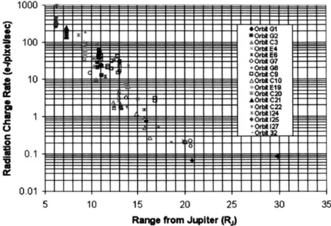
2-3 Galileo SSI count rates by Klaasen et al. (2003) . . . . 45
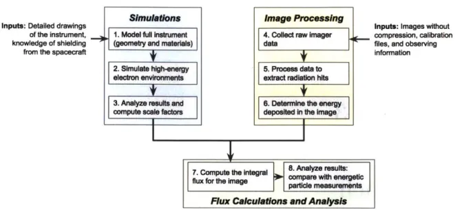
3-1 High-level block diagram of the technique developed . . . . 48
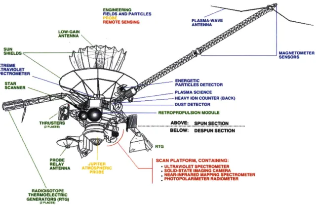
3-2 Diagram of the Galileo spacecraft . . . . 49
3-3 Example macro file for a Geant4 simulation. . . . . 52
3-4 Sample results from Geant4 simulations on an 800 x 800 pixel array 53 3-5 Diagram of the solid angle and area for a generalized flux calculation. 56 3-6 Computing scale factors and integral flux . . . . 58
3-7 Photograph of the Galileo EPD . . . . 59
3-8 Schematic of the EPD telescope heads and the overall EPD configuration 60 3-9 Galileo EPD >11 MeV integral flux . . . . 61
4-1 Photograph of the SSI instrument . . . . 64
4-2 Labeled diagram of the basic elements of the SSI instrument from [131. 64
4-3 Layout of the Galileo SSI CCD . . . . 65
4-4 Modeled SSI instrument with labels of the key components . . . . 66
4-5 Combined calculated scale factor as a function of energy for the SSI. . 68 4-6 Comparison of total exposure times for SSI compression types. . . . . 70 4-7 SSI image processing flow diagram . . . . 71 4-8 Conversion from DN to energy deposited for the SSI gain states . . . 73
4-9 Raw images of SSI observation 3926r. . . . . 75
4-10 Example of radiation extraction from a line in an SSI image . . . . . 76
4-11 Processed image of 3926r . . . . 78
4-12 SSI results compared with the Galileo EPD >11 MeV integral flux . . 80 5-1 Photograph and labeled diagram of the Galileo NIMS instrument . 82 5-2 NIMS detector spacing, materials, and wavelength detection ranges 83
5-3 Annotated visualization of the NIMS CAD model . . . . 84 5-4 CAD model of the NIMS focal plane assembly . . . . 84
5-5 Percentage of particles from simulation that reach NIMS detectors as a function of energy . . . . 85
5-6 NIMS FASTRAD ray tracing results for an individual detector (#16). 86
5-7 NIMS radiation rates by detector . . . . 88
5-8 Calculated fluxes from NIMS observations compared to the EPD . . . 89
6-1 Radiation rate extraction comparison to the literature . . . . 93 6-2 Comparison of the choice of DN threshold for radiation detection . 94 6-3 Comparison of the calculated SSI fluxes to the EPD and to GIRE2 96
6-4 Comparison of the calculated SSI and NIMS fluxes to the EPD and to
G IR E 2 . . . . 97
6-5 Histograms of the energy deposited for each energy simulation . . . . 98 6-6 Comparision of the kinetic energy of particles at the detector and the
7-1 Juno payload system overview . . . . 100 7-2 Europa Clipper system overview . . . . 102 7-3 Earth integral electron flux as a function of L-shell and energy . . . . 105 7-4 Comparison of traditional (chemical) and electric propulsion orbit
tra-jectories to G EO . . . . 106
A-i Diagram of the solid angle and area for a generalized flux calculation. 110
D-1 Timing of the SSI frame sequence . . . . 125 D-2 Residual glow in a SSI image even after the target has been removed. 127
List of Tables
1.1 Comparison between Earth and Jupiter. . . . . 1.2 High-energy particle populations and their radiation effects 1.3 High-energy measurements made at Jupiter . . . .
3.1 Simulation parameters used in Geant4 particle simulations.
4.1 SSI Geant4 simulation results . . . . 4.2 SSI calculated scale factors . . . . 4.3 SSI gain states for converting DN to energy deposited . . . 4.4 SSI observation 3926r parameters. . . . .
C.1 C.2 C.3 C.4 C.5
SSI Geant4 Run 1 . . . . SSI Geant4 Run 2 . . . .
SSI Geant4 Run 3 . . . . SSI Geant4 Run 4 . . . .
SSI Geant4 Run 5 . . . .
D.1 Imaging modes available for the SSI . . . .
19 23 26 51 67 69 73 77 . . . 122 . . . 123 . . . 123 . . . 124 . . . 124 . . . 126
Acronyms
CCD Charge-coupled Device
CMOS Complementary Metal-oxide-semiconductor
DN Data (or Digital) Number
EDR Experiment Data Record EPD Energetic Particle Detector
ESD Electrostatic Discharge
eV Electron-Volt
GEO Geostationary Earth Orbit
GIRE2 Galileo Interim Radiation Electron Model Version 2 GOES Geostationary Operational Environmental Satellite
HGA High-gain Antenna
IESD Internal Electrostatic Discharge
MCP Micro-channel (or Multi-channel) Plate NIMS Near-Infrared Mapping Spectrometer
PDS Planetary Data System
SSI Solid-State Imaging TID Total Ionizing Dose
Chapter 1
Introduction
1.1
Background
Harsh radiation in the form of ionized, highly energetic particles is part of the space environment. These particles sweep through the solar system in the solar wind and solar storms, are ejected from supernovae, and are also trapped as belts in planetary magnetic fields. A planetary magnetosphere is the region of space surrounding the planet in which the physical phenomena of electrically-charged particles is controlled by the magnetic field. The charged particles can affect spacecraft and satellites or-biting the planet.
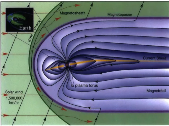
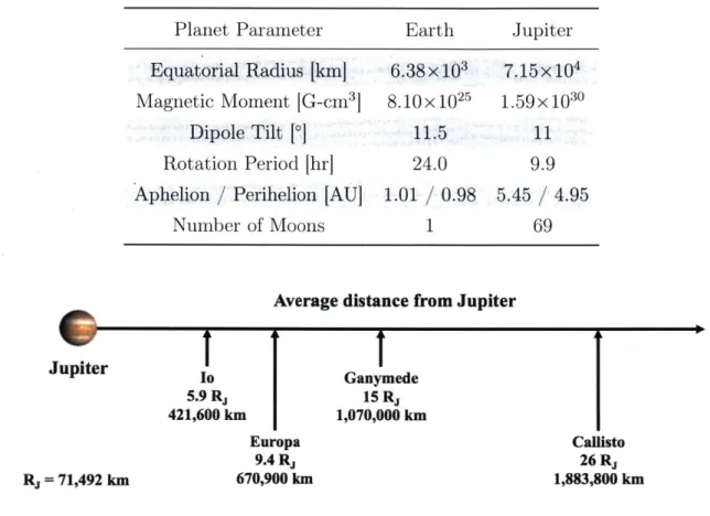
Jupiter's magnetosphere is the largest and strongest of any planet in the solar system. Similar to Earth, Jupiter is approximately a magnetic dipole with a tilt of ~111[46, 70], but Jupiter's magnetic field strength is more than an order of magnitude larger than Earth's and its magnetic moment is ~19,000 times larger [6, 96]. The magnetic field at the equator is proportional to the magnetic moment divided by the cube of the radial distance. Therefore, Jupiter's magnetic field is proportionally about twenty times stronger than Earth's magnetic field. Table 1.1 summarizes the comparison between Jupiter and Earth. The larger field strength means that Jupiter's magnetosphere can contain significantly more charged particles than Earth. Looking at Figure 1-1, the bow shock extends about 84 Rj towards the Sun (where Rj = 71,492 km is the radius of Jupiter), and the magnetotail can extend almost as far
1.o plasma torus
Solar windMagnetotal 1,500,000/
Figure 1-1: Structure of the Jovian magnetosphere. The magnetosphere is the domi-nating influence on energetic particles in the purple region. Earth's magnetosphere, shown in the top left corner, can fit inside Jupiter's radius. Image source: [5].
in the other direction as Saturn's orbit (~50-1000 Rj, or up to -71 million km)
[69, 77]. Jupiter's magnetosphere is thought to be powered by a liquid dynamo
circulating metallic hydrogen. Eruptions of sulfur and oxygen from the Galilean moon Io's volcanoes form a cold torus that rotates with Jupiter at 5.9 Rj, generating ions
through collisions and ultraviolet radiation, altering the dynamics of and supplying mass to the magnetosphere [63, 70, 97]. Figure 1-2 shows the relative locations of the Galilean moons of Jupiter. The particle number density of the plasma in the Jo
torus is about 2,000 particles per cubic centimeter and the effects from Jo's plasma torus extend out to ~50 Ri [69]. At Earth, the only internal source of plasma is the
ionosphere, so the cold plasma population falls off exponentially to just a few particles
per cubic centimeter at 4-5 RE (1 RE = 6,371 km).
The rotation rate of Jupiter (-10 hours) is much faster than that of Earth (24 hours). The fast rotation at Jupiter, coupled with the strong magnetic field, forces
Table 1.1: Comparison between Earth and Jupiter. The Jupiter is from last reported count by [1021.
number of moons listed for
Planet Parameter Earth Jupiter Equatorial Radius [km] 6.38 x 10 7.15x i04
Magnetic Moment [G-cm3 8.10x 1025 1.59x 1030
Dipole Tilt [0] 11.5 1
Rotation Period [hr] 24.0 9.9 Aphelion / Perihelion [AU] 1.01 / 0.98 5.45 / 4.95
Number of Moons 1 69
Average distance from Jupiter
Io 5.9 Rj 421,600 km Europa 9.4 Rj 670,900 km
I
Ganymede 15 R, 1,070,000 km Callisto 26 Rj 1,883,800 kmFigure 1-2: Relative locations of the four Galilean moons of Jupiter. The distances are to scale with the size of Jupiter in the image. Note: There are four smaller, inner moons (Metis, Adrastea, Amalthea, and Thebe) at 1.8-3.1 Rj that are not pictured. in the magnetosphere co-rotates at velocities much higher than a spacecraft's orbital velocity. This is the opposite at Earth, where (at low altitudes) spacecraft orbit faster than the ionospheric plasma. The co-rotation at Jupiter breaks down around 20 Rj [36]. The magnetic field tilt and rotation rate cause the plasma disk to fluctuate so that at a given location plasma and radiation parameters vary significantly during a 10-hour period.
The Jovian radiation environment is dominated by trapped high-energy electrons. The high-energy electron spectra extends to much higher energies (>10 MeV) 1 than the spectra found in Earth's magnetosphere [15, 32, 33, 47]. At Earth, the most
'An electron-Volt (eV) is the amount of energy gained (or lost) by the charge of a single electron moving across an electric potential difference of one volt. 1 MeV = 106 eV.
Jupiter
Rj= 71,492 km
71 A
extreme electron environment is at the outer Van Allen belt (~4-5 RE from Earth),
where the >1 MeV integral flux is ~ 8.8 x 105 cm-2 S- 1.2 At Jupiter, the >1 MeV
electron flux at 6 Rj is > 1 x 108 cm-2 s-1, which is over two orders of magnitude greater than at Earth, extending up to energies of 100 MeV and above [36, 46].
Figure 1-3 compares the electron and proton integral fluxes in Jovian orbit (at Europa) and in geostationary Earth orbit (GEO).
E 0 0) 0 10 10 10 -108 106 105 101 10 -102 10 1U 0.1 1 10 100 1000 Energy [MeV]
Figure 1-3: Comparison of the Jupiter (red) and Earth (blue) electron and proton spectra. The electron and proton spectra for Jupiter are using the GIRE2 model (see Section 1.3.2) at 9.5 Ri (at Europa). The Earth spectra is found using the AE-8 and AP-8 models at solar maximum at 6.6 RE (at GEO) [100, 112].
2Found using the AE-8 model at solar maximum [112].
-- ~ Electrons at Europa (9.5 Rj) -*- Protons at Europa (9.5 Rj) -0- Electrons at GEO (6.6 RE)
-.- Protons at GEO (6.6 RE
1.2
Characterizing the Jovian Radiation Environment
1.2.1
Science Motivation
Determining the composition of energetic particles is critical to our scientific under-standing of the composition, structure, and dynamics of the magnetosphere. Increased temporal coverage and spatial measurements can improve current environment mod-els, which are currently defined by limited data (see Section 1.3).
High-energy electrons affect the Jovian satellites (moons). The energetic electrons are a major contributor to exogenic processes, which affect the albedo and surface chemistry of the moon
[25,
80, 89]. MeV electrons can penetrate through atmospheres, physically and chemically weathering the surfaces of moons. The penetration depths depend on the particle type, particle energy, and material, with particle doses at depths up to a few micrometers in rocky surfaces dominated by ions and at depths greater than ten micrometers by electrons [61, 62, 88]. The electrons are tens of keV to >25 MeV. The effects extend below the surface layer and are relatively permanent. High-energy electrons can drive surface chemistry by ionization that catalyzes chemical reactions, which has direct impacts on the astrobiological potential of a satellite. Since metabolic reactions within living cells depend on chemical energy, it has been suggested that the Europa subsurface ocean has a high potential for sustaining biological activity if some oxidation-reduction chemistry is present [25, 52]. It is likely that Europa's briny subsurface ocean is a reducing environment and the irradiation of a surface by bombardment of charged particles leads to oxidation of the surface [28, 801.1.2.2
Engineering Motivation
Knowledge of the high-energy radiation environment impacts spacecraft mission de-sign, operations, and lifetime. Mission architectures are affected by trading mission lifetime against more desirable science that requires orbits closer to the planet with higher radiation exposure. For example, the Europa Clipper mission flower-petal
mil metric 100,000
Al [il<~1 m
1MOW (g/CM2)
-- e-ml ....~~~c- I <~O.1 mm3-i
E 1000 <-10 -1- p-m < <-10 mm
i100
Elm I r <-1mm c 0.1mm <-10 um 0.1 <-10 kA 0.01 - - -0.01 0.1 1 10 100 1000 Energy (MeV)Figure 1-4: Electron (solid) and proton (dashed) penetration depth in aluminum for a range of energies (0.01 to 1000 MeV). For 100 mils (2.54 mm) of aluminum, protons must have energies above about 1 MeV and electrons must have energies above about
20 MeV to penetrate. Image source: Garrett and Whittlesey (2012) [44].
orbit is specifically designed to maximize science and mission life but minimize radi-ation exposure during the orbit [91]. For the Galileo spacecraft, during the nominal mission, the Solid-State Imaging (SSI) instrument only opened its shutter and took images when the spacecraft was greater than approximately 9 Rj from Jupiter to reduce radiation damage. When the mission was extended (three phases, from 1997 to 2003), the mission operators took greater risks, using the SSI instrument at 5.8 Rj, where the radiation environment is more intense.
The risk of anomalies and degradation to spacecraft are increased in high-energy electron environments (e.g., [8, 40, 54]). Internal (or bulk) charging occurs when MeV electrons penetrate satellite shielding materials and deposit charge on internal spacecraft components. For a spacecraft wall with a thickness of 100 mils (2.54 mm) of aluminum (typical for an Earth-orbiting spacecraft), electrons need energies in the range 0.5-5 MeV to penetrate, and protons need energies of 10-100 MeV (see Figure 1-4 from Garrett and Whittlesey (2012) [1-41-4]). If the component's resistivity is high, the rate of charge build-up can overcome the charge leakage rate of the material.
Table 1.2: Key effects of radiation on spacecraft and the high-energy particle popu-lations that cause the radiation effects.
Radiation Effect High-Energy Particles RadiatiQn dose, dose rate 100 keV - 50 MeV electrons
1 MeV - 100 MeV protons
Surface charging, ESD 1 keV - 1 MeV electrons Single event effects 1 - 100 MeV protons
>1 MeV/Nuc. heavy ions Internal charging, IESD 1 - 10+ MeV electrons
The induced electric field may then exceed the breakdown threshold for the material, causing electrostatic discharge (ESD) in the material
[8,
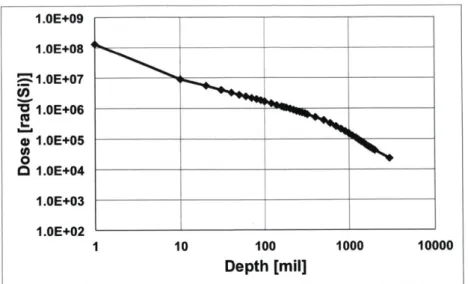
38, 43, 117]. This can lead to anomalies such as component failures, degradation of sensors and solar panels, and serious physical damage to materials. Internal electrostatic discharge (IESD) can happen as a result of electron charges buried in dielectrics or on floating metals inside the spacecraft.Total ionizing dose (TID) is a result of long-term radiation absorption and can lead to undesirable effects such as electron-hole pair production, transport, and trapping in the dielectric material. The total accumulated dose depends on orbit parameters (altitude, inclination, eccentricity), spacecraft orientation, and time. The integrated particle energy spectrum (fluence as a function of particle energy) is used to compute the TID. Figure 1-5 shows the dose depth curve for the Galileo mission as predicted by Galileo Interim Radiation Electron model version 2 (GIRE2). As TID increases, material and component degradation increases, leading to reduced functionality and greater susceptibility to failure. There is also evidence that dose rate affects the TID; electron-hole pair production, transport, and trapping in dielectrics can be more pronounced at lower dose rates (see Chen et al. (2010) for information on "enhanced low dose rate sensitivity" (ELDERS) and references therein [24]).
Increased information about the environment can supplement and refine models that are used for spacecraft design [33, 36]. The survivability and lifetime estimates
I.0E+09 I.0E+08 I.OE+07 U, 1.0E+06 0 1.0E+05 0 O 1.0E+04 1.OE+03 I.OE+02 1 10 100 1000 10000 Depth [mil]
Figure 1-5: Dose depth curve for the Galileo mission by GIRE2. Data are from I. Jun at NASA/JPL.
through orbit 35, as predicted
are developed based on the anticipated environment, influencing part selection (ra-diation tolerant or not), redundancy, shielding design (thickness, material, location), and software development (scrubbing, self-inspection, or not). This leads to signifi-cant impacts on mission cost and schedule, affecting the data that can be returned. For more information about mission design considerations in radiation environments, see Garrett and Whittlesey (2012) [44].
1.3
Particle Measurements at Jupiter
1.3.1
Limited High-Energy Electron Data
High-energy particle information about the Jovian magnetosphere is limited, both spatially and temporally. Table 1.3 shows a list of the spacecraft that have taken high-energy electron measurements at Jupiter. We limit the list to instruments capable of measuring >1 MeV electrons because it is the dominant species at Jupiter and the focus of this thesis. Figure 1-6 shows a plot of the orbit paths of the spacecraft that have recorded high-energy particle measurements with respect to Jupiter. Pioneer 10 and 11 and Voyager 1 and 2 made measurements during flybys in the 1970s and 1980s, respectively [110, 111, 113, 1141. For the most part, the information about the Jovian
environment comes from the Galileo spacecraft Energetic Particle Detector (EPD)
[116].
A top-down view of the Galileo orbits when the EPD made measurements can be found in Figure 1-7. While there were 35 orbits from -5 Rj to over 100 Rj, the Galileo orbit was nearly equatorial around Jupiter, remaining within 5' of the equatorial plane of Jupiter (see Figure 1-6). The axis of the magnetic field is tipped about eleven degrees from the planet's rotation axis, which causes Galileo to cross the magnetic equator roughly every five hours (Jupiter's rotation period is ten hours).10 5-cc 0 -5--10 0 --- --- --- - --- -- -- ---Pioneer 11 Pioneer 10 oyager-Woilo orbite Juno perijove 5 10 15 20
Figure 1-6: Map of the trajectories of spacecraft that have made high-energy mea-surements of Jupiter's magnetosphere in the magnetic dipole frame. The Pioneer 10 and 11 flybys are plotted in green. The Voyager 1 and 2 flybys are in red. The Galileo orbits are in blue. The first Juno perijove is in purple, for reference. Image source: N6non et al. (2018) [84].
Table 1.3: Spacecraft that have made high-energy (>1 MeV) electron measurements at Jupiter. The instruments and energy ranges for each spacecraft are provided.
Spacecraft Instruments Electron Measurements
Pioneer 10 [110] Geiger tube telescope (GTT) >0.06, 0.55, 5, 21, 31 MeV Pioneer 11 [111] Trapped radiation detector >0.16, 0.26, 0.46, 5, 8, 12,
(TRD) 35 MeV
Electron current detector (ECD) >3.4 MeV Voyager 1 [113] Cosmic ray telescope (CRT) 3-110 MeV Voyager 2 [1141
Galileo [116] Energetic particle detector >0.238, 0.416, 0.706, 1.5,
(EPD) 2.0, 11.0 MeV
-Sun-Oriented Orbit Trajectory Primary Mission
Extended Mission 1: GEM
E'xtenided Mission 2: GiM
Orbits of the Galilean Moons
Sun
-50 0
X [RJ]
50 100
Figure 1-7: Polar view of the locations where Galileo EPD measurements were made in a sun-oriented frame (local time with Jupiter). Jupiter is the black dot in the center (to scale) and the four rings around it are the locations of the four Galilean moons. 100 80 60 40 20 0 -20 -40 -60 -80 -1'U --100
1.3.2
Jovian Radiation Models
The first comprehensive model of the Jovian environment, which was the standard for decades, was the Divine and Garrett (D&G) model in 1983, which is built on empirical data from the Pioneer and Voyager spacecraft [36]. The D&G model was updated in 2005 to include synchrotron measurements from Earth-based observato-ries [47]. Presently, there are two models that are used as the standard. The Jovian Specification Environment (JOSE) model [104] by ONERA3 in France, which is based on the Salammb6 theoretical code [103] in combination with data from the Galileo EPD. The Galileo Interim Radiation Electron (GIRE) model combines the Galileo EPD dataset with the original D&G model (good coverage at R3 < 8 from the
Pio-neer and Voyager spacecraft) and synchrotron observations to estimate the trapped electron radiation environment
[34].
The GIRE2 model addresses discontinuities at the boundary between the GIRE and D&G model and extends the model from ~16 Rj up to -50 Rj144,
45]. GIRE2 is the standard used in the United States and is the model used for comparison in this thesis. Table 1.4 provides an overview of the models.1.3.3
Juno and Europa Clipper Missions
Juno, a NASA spacecraft that entered Jupiter orbit in July 2016, measures Jupiter's composition, gravity field, magnetic field, and polar magnetosphere. Nominal science operations started in December 2016. The science phase (altered from the original plan due to an early issue with the propulsion system) consists of 12 science perijoves (14 total perijoves) before the nominal end of mission in July 2018. An extended mis-sion through July 2021 has recently been announced.4 The Juno spacecraft orbits over the poles (90 +10' inclination) with a highly elliptical orbit, lasting approximately 53.5 days. The elongated orbit means that apojove reaches a distance of around 8 million kilometers, passing through Jupiter's magnetotail. Figure 1-8(a) shows the
30ffice National d'Etudes et de Recherches A6rospatiales (ONERA) is the French national aerospace research center.
Table 1.4: Overview of Jovian radiation models. Model Name References Description and Comments
Divine and Divine and First comprehensive model of the radiation Garrett (D&G) Garrett, 1983 and plasma environment around Jupiter,
Empirical, from Geiger tube telescope (GTT) on Pioneer 10 and 11, and from the cosmic ray telescope on Voyager 1 and 2. D&G, updated Garrett et al., Includes data from Earth-based observations
2005 of the Jupiter synchrotron emissions Jovian Specific ONERA, Based on Salammb6 theoretical code in Environment Sicard-Piet et al., combination with data from the Energetic
(JOSE) 2011 Particle Detector (EPD) on the Galileo
spacecraft
Galileo Interim Garrett et al., Empirical model, uses 10-min averages from Radiation 2002 and 2012; de the EPD on Galileo, V2 addresses
Electron (GIRE) Soria-Santacruz discontinuities at the boundary between and GIRE2 et al., 2016 GIRE and the D&G models and extends
from -16 Rj to ~50 R3.
tilt of Juno's orbit relative to Jupiter as the orbit precesses over time. the closest approach ranges from 4,200 km to 7,900 km.
At perijove,
Measurements of the high-energy electron environment from a polar orbiter would greatly increase the spatial data coverage. Juno is equipped with detectors that can measure a maximum of 1 MeV for electrons and 3 MeV for protons. While these detectors cover the Juno primary science objectives, they do not cover the higher en-ergies of concern (radiation dose, single event effects, internal electrostatic discharges) of up to 30 MeV electrons and 100 MeV protons, severely limiting the accuracy of total mission dose measurements. See Figure 1-9 for the energy detection ranges for Juno's Jovian Auroral Distribution Experiment (JADE) and the Jupiter Energetic-particle Detector Instrument (JEDI) compared to the energy ranges of concern for radiation-related effects.
A technique to extract high-energy electron information from science imagers al-ready on Juno could yield important radiation environment information that would otherwise be unreported. Juno has three instruments that are charge-coupled devices
1u I -3 I-0 XI 0* U) 0 0O .0 'U 0 10 -20 - -30- -40- -50--60 120 Joi PJ06 PJlo PJ15 PJ20
PJ25 Orbits are colored by P according to longitude grid used by Nav: Blue = Orbits 1 & 3-5 (yields initial 90-deg spacing) Brown = Orbits 6-9 (45-deg spacing)
PJ30 Green = Orbits 10-17 (22.5-deg spacing)
Magenta = Orbits 18-33 (11.25-deg spacing
pJ34 Purple = Orbits 34-35 (extra and deorbit)
-I--100 80 60 40
East/West Distance about Pole Axis (RJ)
20 0
(a) Juno orbit paths as of June 2018.
(b) Europa Clipper orbit plan.
Figure 1-8: Orbits of Juno as of June 2018 and the plans for Europa Clipper orbits on the top and bottom, respectively. Original images are from [16] and [49]; they have been annotated for clarity.
(CCDs): Juno Color Camera (JunoCam), the Advanced Stellar Compass (ASC), and the Stellar Reference Unit (SRU). Juno also has an Ultraviolet Spectrometer (UVS) that has a micro-channel (or multi-channel) plate (MCP) detector. Each of these instruments presents an opportunity to extract environment information and there are ongoing attempts to do this (see Section 2.4.1).
Europa Clipper, currently in Phase B of design, is a NASA spacecraft designed to assess the habitability of Jupiter's icy moon, Europa. Europa Clipper will orbit Jupiter rather than Europa directly to avoid the high-radiation environment close to Jupiter (see Figure 1-8(b)). On closest approach, Europa Clipper will come within 25 to 100 km of the surface of Europa. There are about 45 flybys of Europa planned for the 3.5-year mission. The main lifetime limiting factor is high-energy radiation [91].
At the time of writing, there are no instruments on Europa Clipper dedicated to MeV particle detection. There has been a proposed Radiation Monitoring System (RMS) that would include a charge monitor and dosimeters for TID, but its capability of providing electron spectrum measurement is being defined. There are instruments that are sensitive to MeV radiation: the Ultraviolet Spectrograph (UVS), Mapping Imager Spectrometer for Europa (MISE), Europa Imaging System (EIS), and MAss SPectrometer for Planetary EXploration (MASPEX). Europa Clipper will also have star scanners. Since these instruments are sensitive to MeV radiation, they could yield information about the high-energy radiation environment.
In summary, to gain a better understanding of the Jovian radiation environment, from both a science and engineering perspective, we need more data: greater orbit diversity of measurements (spatial and temporal coverage and energy range), more exposure time, and a larger area for evaluation (pixels, detector area). Juno and Europa Clipper have orbits that, if higher energy (>1 MeV) particle measurements were taken, would significantly improve the spatial and temporal knowledge of the Jovian magnetosphere.
I.
I
Europa Clipper
Juno JAME JEDI
No high-energy particle
measurements planned
g Polar orbit, minimal coverage of radiation dose energies I
Euw nso Paticle Detec
Galileo Plasma Science Plasma Analyzer *ECT OTT 101 102 10 104 105 Energy [eV]
itor -Equatorial orbit
CRT Flybys only
ECD TFlybys
only
TRD
106 108 109
Surface charging: I keV -1 MOV Radiation dose: 100 keV - 50 MeV Internal charging: I MeV - 10 MeV Figure 1-9: Energy ranges covered by instruments on spacecraft to Jupiter. The shaded regions correspond to the energy ranges of concern for specific radiation ef-fects: the radiation dose and dose rate risks in blue, internal charging and internal electrostatic discharge (IESD) risks in pink, and surface charge risk in green. Pio-neers and Voyagers made high-energy electron measurements in the zones of concern, but those missions were only flybys, resulting in limited temporal and spatial mea-surements. Galileo EPD made measurements over a period of 35 orbits, mainly equatorially around Jupiter. Juno orbits over the polar region of Jupiter, but has limited high-energy detection capabilities. For the Europa Clipper mission, currently in development, there are no dedicated high-energy particle measurements planned.
1.4
Motivation for Developing a Technique Using
Sci-ence Imagers
Energetic particle detectors are not always included on spacecraft due to resource constraints (e.g., cost, complexity, schedule). From a sampling of energetic particle detectors designed for Earth orbit, Jupiter orbit, and interplanetary medium, we find commonality in design due to similar engineering constraints and scientific goals. We find that the average mass is in the 10's of kilograms, the average power needs are in 10's of Watts, and the sizes range significantly (depending on the types and energies of particles for detection) from about 10 to 40 cm in each dimension [59]. The amount of electronics can be significant as well, and the need for low-power, densely packed,
Voyagers 1 & 2;
Pioneers 10 & 11
Swaoft Perticle Deft
radiation-tolerant components leads to extensive use of custom integrated circuitry. Due to the significant mission costs and time it takes to reach the outer solar system, spacecraft missions to Jupiter are infrequent (see Sec. 1.3). In addition, orbiters are even more challenging: it's much more costly to orbit than to do a fly-by in terms of the delta-V needed. Using estimates of mission costs and wet masses of missions to the outer solar system (plotted in Figure 1-10), we find that the approximate cost per kilogram to the outer solar system is ~$500,000/kg in FY2000 dollars. In contrast, the average cost to send mass to low Earth orbit is -$20,000/kg.
In the absence of energetic particle detectors, we explore how existing hardware, common to missions to the outer solar system, can be used as sensors of the high-energy electron environment. We focus our study on scientific imaging instruments ("imagers") for two reasons: (1) scientific imagers are common to exploration space-craft, such as those designed for Jupiter and other exploratory missions, and (2) radiation effects are a well-observed and studied phenomena in imagers [30, 571. We focus on solid-state devices, using semi-conducting detecting materials, where the
4000 U) 0 0 0 Cassini 3000 Pioneers 2000
New Horizons Galileo
1000 *DJuno Voyagers Ulysses U 1000 2000 3000 4000 5000
Wet Mass [kg]
Figure 1-10: Approximate launch cost in FY2000 dollars per kilogram for missions to the outer solar system. The best fit line has a slope of -$500,000/kg in FY2000 dollars.
sensitivity to radiation manifests as noise
[57].
There are well-documented (though limited) techniques for extracting radiation "hits" for proton noise, which we build upon to develop a novel method to identify electron noise. These techniques are discussed in Chapters 2 and 3.This technique could be used in other environments (e.g., Earth orbit, or inter-planetary) and could use other types of imagers (e.g., star cameras). For example, for an astrophysical observatory with sensitive detectors, such as the Transiting Ex-oplanet Surveyor Satellite, the final orbit may be relatively benign with regards to radiation, but the spacecraft must still traverse the Earth's radiation belts, providing the possibility of additional radiation measurements. We discuss other applications in Chapter 7.
1.5
Thesis Contributions
The goal of this thesis is to extract quantitative information about the high-energy (>1 MeV) electron environment at Jupiter using existing technologies on-board space-craft. We propose using science imagers, which are sensitive to MeV electrons that are recorded as noise on the detector and detailed simulations of the instrument's response to high-energy electrons to determine the energy and flux of electrons in the environment.
We develop the technique using data from the Galileo spacecraft, which provides an excellent opportunity for analysis, since there are both imaging instruments and an energetic particle detector that can be used for validation. We use the Galileo Solid-State Imaging instrument, which is an 800 x 800 pixel CCD, to demonstrate the method. We identify and extract the electron radiation noise in the flight data and compare the noise to charged particle transport simulations in Geant4, a charged particle transport code
[2],
to determine the energy sensitivity of the instrument. We compute the integral flux and the results are then compared to the Galileo EPD for validation. We demonstrate that the technique is useful for a general imager by applying the method to another imager: the Galileo Near-Infrared MappingSpec-trometer (NIMS), which is a focal plane array spectrograph with seventeen individual photovoltaic diodes, also showing agreement with the EPD.
In summary, this thesis makes the following contributions:
1. Develops an approach for combining simulations using detailed mechanical and materials models of imaging cameras along with experimental image analyses to obtain particle energy measurements.
2. Creates a process for extracting electron radiation hits in an imager.
3. Demonstrates and validates a generalized procedure for calculating the environ-ment integral flux from an imager.
4. Establishes guidelines for pre-flight testing and calibration, as well as in-flight operational procedures to use an imaging instrument for energetic particle mea-surements, including specific recommendations for the Juno and Europa Clipper missions.
1.6
Thesis Organization
In Chapter 1, we discussed the space radiation environment, focusing on the Jovian energetic electrons. We described the models that are used, the particle measurements and physics the models are derived from, and the effects of radiation on spacecraft. We discussed the need for in-situ particle flux and energy information, but illustrated the challenges with including dedicated energetic particle measurements. In Chapter 2, we summarize how imagers work and explain how high-energy charged particles affect imagers. We discuss previous work using imagers to detect radiation, reviewing the relevant literature. Chapter 3 describes the technique developed for calculating a flux measurement from an image, using detailed models of an imager and extracting radiation from a raw image. In Chapters 4 and 5, we analyze the Galileo SSI and Galileo NIMS instruments, respectively. We simulate high-energy particle transport in models of the instruments and extract high-energy radiation signatures from the raw images. We compare the computed fluxes to the Galileo EPD. We discuss the sensitivity of the technique to noise and other factors in Chapter 6 and compare the
results to GIRE2. Chapter 7 describes how the technique can be applied to other missions and different environments and directions for future work.
Chapter 2
Literature Review
In this chapter, we will explain how imagers are sensitive to high-energy electrons and provide context for this work by reviewing previous efforts using imagers to detect radiation.
2.1
Solid-State Detectors
A solid-state detector (or a semiconductor-based device) is a photosensitive device that converts incoming photons into electric charge. The detecting medium is a semiconductor material such as a silicon or germanium crystal. Solid-state detectors include three main types of devices in space-based imaging: charge-coupled devices (CCDs), complementary metal-oxide-semiconductors (CMOSs), and infrared focal plane arrays. The imagers can be any shape, with hundreds to millions of imaging elements ("pixels"). Charge generation takes place at the semiconductor body of the device in two ways: (1) by the photoelectric effect, where photons create free electrons by promoting electrons into the conduction band, and (2) by ionizing energy loss, where an energetic charged particle creates an electron-hole (e-h) pair. The generated electric current is converted to a digital signal when the device is read out
[57]. Section 2.2 explains more thoroughly the effects of energetic electrons.
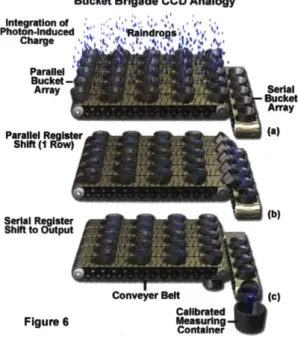
The CCD is one of the most common types of solid-state imagers due to its low noise operation, high resolution, precise image geometry, and stability [18, 57]. CCDs
Bucket Brigade CCD Analogy
Charge ~1
Conveyer Belt (C)
Figure 2-1: CCD operation and readout are analogous to a rain bucket brigade. Photons are collected like rain into individual pixels like buckets. Each pixel converts the photons into electrons. The pixels are read out line by line, like shifting the
buckets and collecting the rain. Image source: 1311.
typically consist of a matrix of potential wells, or pixels. Free electrons generated
within the silicon lattice by the passage of charged particles, such as those found in the
space environment, are stored in the individual pixels. Then, the charge pattern must be transferred out of the CCD, which is done in a controlled manner by modulating the gate potential across the CCD gates (thin conducting strips). The time reference to which the potential changes are synchronized is called a clock cycle. The end pixel or line of pixels is transferred to a special pixel array, called the serial register. The result is a sequence of charge packets emerging from the serial register, each of which is directly proportional to the photon(s) striking the particular location on the CCD. The final step is to convert the emerging charges into electric signals with preamplifiers on the chip. A commonly used analogy for the CCD serial readout is
the rain bucket analogy, where each bucket (pixel) collects rain (photons, which are
converted to electrons in the bucket), and an entire row is shifted in parallel into a series of reservoirs on a perpendicularly oriented conveyor. The accumulated rain in each bucket is measured in series by pouring the container into a calibrated container
(an analog to digital converter). See Figure 2-1. For more information on general CCD operation, the reader is referred to Janesick (2001) and Ch. 46 of Webster and Eran (2014) [57, 1151. Figure 4-3 shows a diagram of the Galileo SSI CCD, which is an 800 x 800 pixel virtual phase CCD. A virtual phase CCD is an extension of the two phase CCD and is unique in that it requires only a single level of gate metalization to control CCD charge collection and transfer
[58].
For a CMOS detector, each pixel has its own charge-to-voltage conversion elec-tronics, enabling readout for each pixel. The increased electronics lead to less area for photon collection and increased complexity, leading to additional noise. However, CMOS technology is typically less expensive due to the manufacturing process and consumes less power compared to CCDs.
2.2
Charge Generation in Solid-State Detectors
A charged particle passing through semiconductor material, such as silicon, creates electron-hole (e-h) pairs by breaking a covalent bond in the silicon lattice. In a low energy state, the silicon crystal structure consists of atoms tetrahedrally bonded by sharing valence electrons (covalent bonding). A charged particle can break bonds creating "free" electrons and corresponding "free" holes. The electrons and holes are " carriers," or mobile charged particles. The total charge generated is proportional to the energy lost by the charged particle,
Q
oc AE. A charged particle must have enough energy to jump from the valence band to the conduction band. The band gap is dependent on the material, doping, and device configuration. For silicon, the bandgap is Eg = 1.12 electron volts
(eV).
Energetic electrons lose kinetic energy in matter in two ways: (1) through inelastic collisions with orbital electrons in the semiconductor, exciting and ionizing atoms along their trajectory, and (2) at higher energies, through bremsstrahlung radiation, which occurs when the particle is deflected or slowed down in the electric field of a nucleusi, emitting radiation [57, 108]. It is also possible that the electrons elastically
Stopping Power: Electrons in Aluminum 10 2 101 0 100 -.00 CL 10 .
--- Total StoppIng Power
- ~- - Collision Stopping Power
- -Radiative Stopping Power
102 101 100 101 102 10
Kinetic Energy [MeV]
Figure 2-2: Stopping power of electrons in Aluminum with contributions from colli-sional and radiative losses. Data source: [86].
scatter from nuclear and electronic interactions or through nuclear excitation, but these processes are usually negligible and applicable at lower energies [108]. The stopping power dE for a material is a measure of the retarding force on the particle in matter. For electrons, the total stopping power is:
dE) ( dE dE (2.1)
dx total dx collisional dx radiative
The relative importance of each contribution depends on the material (atomic number,
Z) and the energy (E) of the particle.2 The two rates of energy loss are approximately
equal when
(dE/dx)radiative ZE(2.2)
(dE/dx)coisionai 800
So, for Aluminum (Z = 13), the collisional and radiative losses are equal at
approx-imately 60 MeV. A plot of the stopping power for electrons in Aluminum with the contributions from collisional and radiative losses is given in Figure 2-2.
The energy loss of a particle in a shielding medium is a function of the distance
2
Collisional stopping power is proportional to Z and increases logarithmically with energy. Ra-diative stopping power is proportional to Z2 and increases linearly with energy.
traveled and the type and initial energy of the particle. The atomic electrons either experience a transition to an excited state or to an unbound state into the conduction band (i.e., ionization). Nearly all energy loss (99.9%) is converted to electron-hole (e-h) pairs, called "ionizing energy loss" (IEL). The remaining energy is given to nonionizing interactions, including displacing silicon atoms, called "nonionizing energy loss" (NIEL). During IEL, conduction band electrons are collected in the nearest potential well, generating a transient event in an image [30, 57, 75]. Charged particles leave a electron-hole track producing approximately one electron-hole pair for every 3.65 eV of energy absorbed in silicon [57, 76]. The ionizing trail of charge left behind is not a permanent feature and can be erased simply by reading the CCD. This charge deposition by an energetic particle is what this thesis aims to extract from the flight data. More information on the space radiation impacts on imagers can be found in
[57, 105, 118].
2.3
Radiation Identification in Science Images
The majority of the literature on space radiation detection with imagers is with reference to identifying and removing proton and cosmic ray radiation effects. Since the radiation is seen as a nuisance rather than data, anything resembling radiation (which could include other noise sources) is removed aggressively. Anderson and Bedin (2010) and Prod'homme et al. (2012) look at proton damage identification and charge transfer efficiency corrections for Hubble Space Telescope CCDs and Gaia CCDs, respectively [3, 92]. Cresitello-Dittmar, Aldcroft, and Morris (2001) identify warm pixels from the Chandra X-ray Observatory's star camera CCDs. The typical process is to identify radiation and then remove its contribution from the image signal that one is trying to measure. Techniques for identifying and removing radiation include outlier detection, where pixels that are a certain standard deviation above the surrounding pixels are identified and removed, and boxcar averaging in which pixels with more than a few standard deviations above the mean of the box (e.g., a 5 by 5 pixel box) are replaced with the average of the box [105]. The only literature
on identifying or removing electron radiation noise from imagers in space is from a handful of works on Galileo, New Horizons, and Juno. These analyses will be discussed in detail in Section 2.4.1.
2.4
Imagers as Radiation Sensors
There have been a few instances in the literature where effects on an imager have been identified for the purposes of making measurements of the radiation environment.
Earth-based radiation detection. Earth-based imagers have been proposed as sensors for radiation detection [181. For high-energy alphas (a) and protons, Li et al. and Burke et al. (1997) proposed the use of back-illuminated and front-illuminated CCDs, respectively, for charged-particle spectroscopy. They irradiated a large-area front-illuminated imager with a particles with energies up to 5.5 MeV and protons up to 13 MeV. These studies were for diagnostics of inertial confinement fusion implo-sions. They compared the tests to calculations and found agreement, concluding that CCDs could be used for proton and alpha particle spectroscopy [20, 56, 79]. Most recently, Archambault et al. (2008) characterized radiation-induced noise in CCDs that are now being used more frequently for medical radiation therapy, comparing four radiation filtration techniques
[4].
Space-based radiation detection. In Grant et al. (2010, 2012) and Ford and Grant (2012), the Chandra X-ray Observatory advanced CCD imaging spectrometer (ACIS) team developed a technique to use the CCDs as radiation monitors. The Electron, Proton, Helium Instrument (EPHIN) is a particle detector on Chandra to monitor the local high-energy particle environment. Elevated temperatures on board have limited EPHIN's effectiveness as a radiation monitor; the signal is dominated by thermal noise. Given the degradation of EPHIN, the ACIS CCDs are used to measure the environment. The charge transfer inefficiency (CTI) for two of the CCDs (one backside-illuminated and one frontside-illuminated) is measured over time [42, 51, 50]. Grant et al. (2010, 2012) use ACIS CTI measurements from early in the mission and
compare them to the EPHIN data. The algorithm detects CTI threshold crossings and shows good agreement with the EPHIN. This technique is the current state of the art for actively measuring proton radiation using active imaging CCDs.
Shen and Qin (2016) (and references therein) present cosmic ray estimates using spikes in raw solar images from the CCDs on the Solar and Heliophysics Observa-tory (SOHO) Extreme ultraviolet Imaging Telescope (EIT). They computed count rates and find agreement with the Geostationary Operational Environmental Satel-lite (GOES) 11 P6 channel (80-165 MeV) 11011. They employ a median filtering algorithm, which had been shown previously to be effective at identifying cosmic rays [35, 41].
2.4.1
Imagers as Electron Radiation Sensors
Literature on identifying noise in imagers due to electrons can be found from mis-sions in (or flying by) the Jovian environment. In the New Horizons mission, which had an eleven day Jupiter dusk flyby in 2007, Steffl et al. (2012) examine the MeV electrons detected in the background noise of the Alice ultraviolet imaging spectro-graph