https://doi.org/10.4224/20393383
READ THESE TERMS AND CONDITIONS CAREFULLY BEFORE USING THIS WEBSITE. https://nrc-publications.canada.ca/eng/copyright
Vous avez des questions? Nous pouvons vous aider. Pour communiquer directement avec un auteur, consultez la
première page de la revue dans laquelle son article a été publié afin de trouver ses coordonnées. Si vous n’arrivez pas à les repérer, communiquez avec nous à PublicationsArchive-ArchivesPublications@nrc-cnrc.gc.ca.
Questions? Contact the NRC Publications Archive team at
PublicationsArchive-ArchivesPublications@nrc-cnrc.gc.ca. If you wish to email the authors directly, please see the first page of the publication for their contact information.
Archives des publications du CNRC
For the publisher’s version, please access the DOI link below./ Pour consulter la version de l’éditeur, utilisez le lien DOI ci-dessous.
Access and use of this website and the material on it are subject to the Terms and Conditions set forth at
NEF Validation Study: (1) Issues Related to the Calculation of Airport Noise Contours
Bradley, J. S.
https://publications-cnrc.canada.ca/fra/droits
L’accès à ce site Web et l’utilisation de son contenu sont assujettis aux conditions présentées dans le site LISEZ CES CONDITIONS ATTENTIVEMENT AVANT D’UTILISER CE SITE WEB.
NRC Publications Record / Notice d'Archives des publications de CNRC:
https://nrc-publications.canada.ca/eng/view/object/?id=7bc78b8d-fdad-46a5-ba59-e2b12700f4a0 https://publications-cnrc.canada.ca/fra/voir/objet/?id=7bc78b8d-fdad-46a5-ba59-e2b12700f4a0
NEF Validation Study: (1) Issues Related to the Calculation of Airport Noise Contours
Bradley, J.S.
www.nrc.ca/irc/ircpubs
( 1 )
I ssues Related to the
Ca lcu la t ion of Air por t N oise
Con t ou r s
Cont ract Report A- 1505.3( Final)
This report was j oint ly funded by:
I nst it ut e for Research in Const ruct ion, Nat ional
Research Council
and
Transport Canada
This r epor t m ay not be r epr oduced in whole or in par t wit hout t he wr it t en consent of bot h t he client and t he Nat ional Resear ch Council Canada
A1505.3(Final), Page 1
NEF VALIDATION STUDY: (1) ISSUES RELATED TO THE CALCULATION OF AIRPORT NOISE CONTOURS
The contents of this report are the results of analyses carried out by the Acoustics Laboratory of the Institute for Research in Construction at the National Research Council Canada. While they are thought to be the best interpretation of the available data, other interpretations are possible and these results may not reflect the interpretation and policies of Transport Canada.
SUMMARY
This is the first of three reports containing the results of an NEF validation study for Transport Canada. Summaries of the other two reports are included in Appendix 2 of this report.
The NEF_1.7 program is a critical part of the management of airport noise in Canada, and it is extremely important that its validity and accuracy be as good as is reasonably possible. The use of millions of dollars worth of land near airports is determined by the noise level contours from this program. Similarly, the acceptability of land near airports for residential use is determined from the calculated noise contours produced by the NEF_1.7 program. The analyses of this report suggest that improving the detail of the flight path description and developing a more correct excess ground attenuation calculation procedure would considerably improve the NEF_1.7 program. It is therefore essential that the required continuing development of the NEF_1.7 program receive the necessary financial and technical support.
The analyses of this report were focused on the errors associated with predicting noise levels around airports. The related problems of determining acceptable noise level limits and the practical application of these limits will be considered in a second report. These two reports will form the technical background for a final report evaluating the use of the NEF measure to quantify airport noise levels near Canadian airports.
Some of the major technical findings of this report are as follows:
• The NEF_1.7 program is similar to other models such as the Integrated Noise Model (INM) and NoiseMap used in U.S.A. Compared to these two models, NEF_1.7 uses simpler flight path descriptions and a different excess ground attenuation calculation. More sophisticated simulation type models are now being
developed that are potentially more accurate, such as the Swiss model.
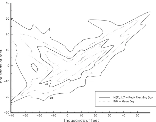
• Comparisons of the NEF_1.7 program with the INM and NoiseMap programs using the same input data from four Canadian airports showed that the NEF contours from the NEF_1.7 program were 60 to 80% larger and NEF values at particular locations were 3 to 4 dB higher. However, it is not known which prediction model agrees best with measured aircraft noise levels. When the complete Canadian approach of using a Peak Planning Day with the NEF_1.7 program was compared with the American approach of using a mean planning day and the INM model, even larger differences resulted.
• Errors in estimating the expected future total aircraft operations could typically lead to 1 dB errors in NEF values and 12% errors in contour areas. Errors from estimating the number of night-time operations would usually be about half as large. Other errors in the estimated input data for future conditions would have smaller overall effects but often quite significant local effects.
• The detail in which the horizontal ground track and the vertical profile of the flight path are described influence the accuracy of the predictions. It is particularly important that the expected
horizontal dispersion of aircraft about the nominal flight track be included in airport noise contour predictions.
• The major cause of differences between the contours produced by the NEF_1.7 program and those from the two American programs is their calculation of excess ground attenuation. Evidence from European research and limited measurements of modern civil aircraft suggest that the most appropriate excess ground
attenuation is intermediate to the NEF_1.7 procedure and the SAE procedure used in the INM and NoiseMap. Data from more
extensive experimental studies are required to determine a better excess ground attenuation calculation procedure. Performing calculations in octave bands would permit more accurate estimates of the propagation of aircraft noise.
• A systematic procedure for relating single event noise measures to combined measures for many aircraft is presented.
• A-weighted SEL values and PNL weighted EPNL values can be related with standard errors of less than 2 dB. Ldn and NEF values were found to relate with errors of less than 1 dB.
• Approximate conversions between various airport noise measures were systematically derived. The largest scatter in these
A1505.3(Final), Page 3
relationships is caused by differences in frequency weightings and time of day weightings.
A1505.3(Final), Page 5
CONTENTS
1.0 Introduction...7
1.1 The Importance of Airport Noise Level Predictions...7
1.2 Content of this Report ...7
2.0 Basic Principles of Airport Noise Measures and Airport Noise Prediction ...9
2.1 Airport Noise Measures...9
2.2 Fundamentals of Airport Noise Prediction ...11
2.3 The Components of Airport Noise Predictions ...13
2.4 Comparison of the NEF_1.7 INM and NoiseMap Programs...15
3.0 Predicting the Number of Aircraft Operations ...17
3.1 Forecasting Future Aircraft Movements ...17
3.2 Predicting the Number of Operations for the Peak Planning Day ...18
3.2.1 The Transport Canada Approach ...18
3.2.2 Analysis Procedures ...20
3.2.3 Average Analyses at All Airports ...22
3.2.4 Recommendations...24
4.0 Comparisons at Four Canadian Airports...27
4.1 Comparison of NEF_1.7 INM, and NoiseMap Results for Similar Input ...27
4.2 Comparison of Results for the PPD and the Mean Day...36
5.0 Sensitivity Analysis ...43
5.1 Noise Level Versus Contour Area Increments ...43
5.2 Total Number of Operations ...45
5.3 Number of Night-time Operations...49
5.4 Stage Length...49
5.5 Number of Chapter 3 Aircraft...51
5.6 Runway Use...51
5.7 Summary...53
6.0 Effects of Details of the Calculation Process ...55
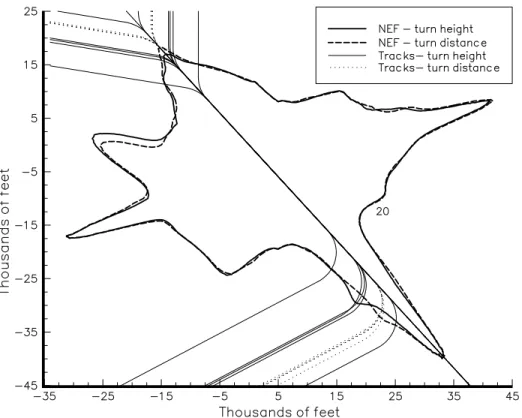
6.1 Turn Rate Versus Turn Radius ...55
6.2 Turn at a Distance Versus Turn at an Altitude...57
6.3 Horizontal Dispersion ...58
6.4 Flight Profiles and Vertical Dispersion ...63
6.5 Grid Spacing and Orientation...65
6.6.1 NEF_1.7 Method...68
6.6.2 SAE Method ...68
6.6.3 Comparison of the NEF_1.7 and SAE Methods ...71
6.6.4 Comparisons with Other Results...72
6.6.5 Effect of Ground Attenuation on Single Aircraft Contours...74
6.6.6 Effect of Ground Attenuation on Overall Airport Contours...77
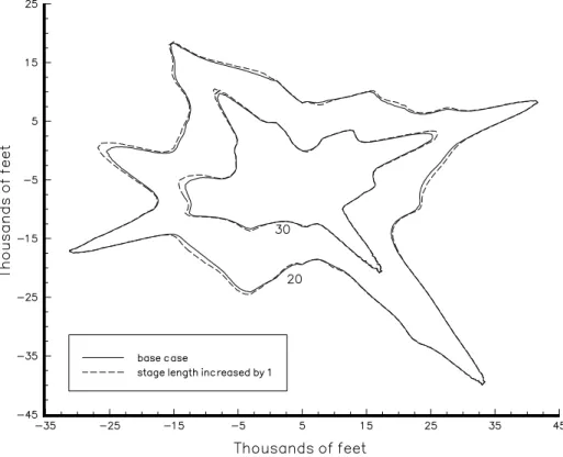
6.7 Stage Length...82
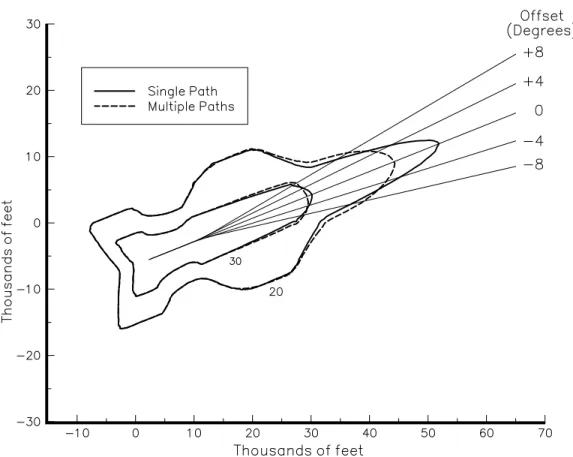
7.0 Comparison of Single Event and Multiple Event Measures ...87
7.1 Procedure for Relating Single Event and Multiple Event Measures ...87
7.2 Example Comparisons of Single Event and Multiple Event Contours ...89
8.0 Comparison of A-weighted and EPNL Based Measures...95
8.1 SEL Versus EPNL Values...95
8.2 Ldn Versus NEF Values...97
9.0 Conclusions ...101
Appendix 1 Approximate Conversions Between Airport Noise Measures ...105
A1.1 Calculation Procedures ...105
A1.2 Comparisons for Full 24 Hour Periods ...111
A1.3 Comparisons for Day Only ...120
A1.4 Influence of Effective Fly-by Duration ...120
Appendix 2 Summaries of Other Reports...123
A2.1 NEF Validation Study: (2) Review of Aircraft Noise and Its Effects...123
A1505.3(Final), Page 7
1.0 INTRODUCTION
1.1 The Importance of Airport Noise Level Predictions
Airports are both a major asset and a liability to nearby communities. They provide jobs to residents, stimulate the local
economy, and provide essential transportation for both passengers and freight. At the same time, aircraft create noisy areas around airports that may not be suitable for residential use. The development of land for residential use is usually more profitable than for other purposes. Thus, there is a conflict between the growth and development of the airport and the development of land for residential use.
Transport Canada provides land-use planning guidelines for areas in the vicinity of airports to assist both aviation planners and those responsible for planning the use of land adjacent to airports. Only
guidelines are provided because in Canada the provinces are empowered to regulate the use of land not under federal jurisdiction via local land-use zoning by-laws. Provinces are free to choose whether to implement these guidelines
Planning guidelines are usually based on predicted airport noise level contours. That is, equal noise level contours are calculated around the airport and a noise level is set above which residential development is considered unacceptable. The process of predicting these noise contours is thus critical to the development of millions of dollars worth of land at each major airport. It is, of course, also critical to protecting residents from excessive levels of airport noise. Therefore, one cannot over-stress the importance of the validity and accuracy of airport noise level
predictions.
There are two parts to the process of resolving land use conflicts around airports. The first part is the purely physical problem of
accurately predicting noise levels around airports. This part of the problem is examined in this report. The other part of the problem concerns the determination of acceptable noise limits and the practical application of these limits. These issues will be discussed in a second report. It is intended that these two reports will form the technical background for a final report evaluating all aspects of the use of the NEF measure to quantify noise levels near Canadian airports.
1.2 Content of this Report
Transport Canada uses the NEF_1.7 computer program to calculate NEF contours around airports. It is therefore of considerable importance to consider the magnitude of various possible errors included
in the complete prediction process involving the NEF_1.7 program. This includes errors in the prediction of the details of future aircraft
operations as well as errors in the estimation of noise levels from specific aircraft operations. The analyses of possible sources of error included in this report were performed largely by systematic manipulation of the input data and by comparisons of results from the Integrated Noise Model (INM) and the NoiseMap programs used in the United States with those from the NEF_1.7 program. Unfortunately, differences between NEF_1.7 and the INM program do not indicate which prediction program is more correct.
Each of the following chapters examines specific aspects of the problem of predicting noise levels around airports. Chapter 2 discusses the basic principles of different approaches to calculating airport noise levels. The errors associated with predicting future numbers of aircraft operations are examined in Chapter 3. In Chapter 4, the calculations of three computer programs (NEF_1.7 INM, and NoiseMap) are compared for four Canadian airports varying in size from small to large. The sensitivity of the NEF_1.7 program to systematic changes in the input data is examined in Chapter 5. Chapter 6 contains analyses of the effects of various details of the prediction programs such as the specification of the complete flight path and the propagation of sound from aircraft to specific receiver points. In Chapter 7, a procedure for relating single event measures to combined airport noise measures is developed.
A-weighted and Perceived Noise Level based measures are compared in Chapter 8. Finally, Chapter 9 presents overall conclusions from the various analyses.
A1505.3(Final), Page 9
2.0 BASIC PRINCIPLES OF AIRPORT NOISE MEASURES AND
AIRPORT NOISE PREDICTION
2.1 Airport Noise Measures
Although there are a variety of airport noise measures, they can be divided into two types: measures of the noise of individual aircraft and measures of the combined effect of many aircraft.
For both types of measures there are different frequency
weightings that cause the noise in each frequency band to be combined with different weighting factors. These frequency weightings are intended to rank the importance of each frequency band in a similar manner to the human hearing system. For aircraft noise, sounds are usually either A-weighted or expressed in terms of Perceived Noise Levels, PNL. The A-weighting curve is an approximation to an equal loudness contour and is widely used in all areas of noise control. The Perceived Noise Level system is more complicated and was specifically developed to rate the noisiness of jet aircraft typical of the 1960’s. These two frequency weighting approaches are compared in Chapter 8 of this report.
Individual aircraft noise measures are either maximum level type measures or integrated measures that represent the integration or sum of the noise energy over a complete pass-by of an aircraft. The most
common maximum level measures are: the maximum A-weighted level (Lmax) and the maximum Perceived Noise Level (PNLmax). They correspond to the maximum level of the aircraft and so represent noise levels from one particular point of an aircraft fly-over. Integrated measures sum the noise energy over a complete fly-over and can also be either A-weighted (e.g. the Sound Exposure Level, SEL) or Perceived Noise Level weighted (e.g. the Effective Perceived Noise Level, EPNL). Because they include the entire pass-by, the integrated measures are a better representation of the total noise radiated by an aircraft.
Both the maximum levels and the integrated measures are
influenced by the directionality of the noise radiated by the aircraft and by the propagation of the noise from the aircraft to the receiver. The interaction of the direct sound and the ground reflected sound can cause considerable attenuation of the total sound from the aircraft at a receiver. This varies considerably with the distance and elevation of the aircraft. Thus, during a complete fly-over the directional radiation of sound from the aircraft and the propagation to a particular receiver is changing continuously in a very complex manner. This detail is lost in the integrated measures which only represent the sum of all these details.
The complete noise climate around an airport is usually described in terms of the combined effects of all aircraft operations over some typical day. Again, these can be based on A-weighted levels or Perceived Noise Levels. Most commonly, the effects of each aircraft are added on an energy basis. That is, the total is just the sum of the noise energy
contributed by each aircraft usually presented as an average for a typical day’s operations. In some cases, the number of events is given more importance and the result is no longer a simple energy sum. Most combined airport noise measures also include various time-of-day weightings. Frequently, time of day weightings are in the form of an additional night-time penalty whereby night-time noise levels are counted as more detrimental than day-time noise levels.
The Noise Exposure Forecast, NEF, used in Canada, and the day-night sound level, Ldn, used in the United States, are two examples of combined airport noise measures that add the contributions of each aircraft on a simple energy basis. The NEF measure is based on the integrated EPNL values of individual aircraft fly-overs and the Ldn is based on the A-weighted SEL values of integrated individual aircraft fly-overs. Both NEF and Ldn include night-time weightings. In
calculating Ldn values, the contribution of night-time SEL’s is increased by 10 dB to represent their expected increased disturbance. In the NEF measure, the night-time weighting is approximately 12 dB.
Two examples of combined airport measures that are not simple energy summations are the quantities used in Switzerland and Germany. The Noise and Number Index, NNI, formerly used in the United
Kingdom and still in use in Switzerland, gives a higher importance to the number of events. Similarly, the German Störindex, or Airport Noise Equivalent Level, gives increased importance to the number of events. For a simple energy summation measure, doubling the number of aircraft operations and halving the energy from each aircraft would not change the total. For the Swiss and German measures, this example would result in an increase in the value of the combined measure.
The major combined airport noise measures are defined in Appendix 1 of this report, and approximate relationships between the measures used in various countries are calculated. The question of which is the most appropriate measure must include consideration of how
people are affected by airport noise. This will be included in a subsequent report.
A1505.3(Final), Page 11
2.2 Fundamentals of Airport Noise Prediction
There are many different airport noise prediction programs that attempt to model a very complex problem with a variety of simplifying approximations. There are approximations to the actual aircraft flight paths, to the production of noise by the aircraft, and to the propagation of the noise to receiver points.
Receiver α2 β2 directional pattern Flight path Ground track h h β1 D2 D1 α1
Figure 2.1: Illustration of the geometry of a simple straight path aircraft pass-by.
Figure 2.1 illustrates the simplest of cases: a single aircraft traveling on a straight horizontal flight path, past a single receiver position. The total noise exposure at the receiver can be obtained by integrating the noise from the aircraft over the complete pass-by. As the aircraft proceeds from left to right in this figure, it gets further and further away from the receiver and hence noise levels tend to decrease. This decrease with increasing distance is first modified by the directional characteristics of sound radiated from the aircraft. That is, aircraft do not radiate noise equally in all directions. The decreased noise levels with increasing distance are also modified by excess ground attenuation which is approximately related to the vertical angle of elevation, β. The further away the aircraft is from the receiver, the smaller the vertical angle of elevation. For example, in Figure 2.1, angle β2 is smaller than angle β1. As this elevation angle β decreases, excess ground attenuation increases. Unfortunately, our knowledge of the directionality of sound radiation from various aircraft and of the excess ground attenuation is not
or thermal inversion also affect sound propagation. Thus, modeling the integration of aircraft noise over a single straight line pass-by, to provide either EPNL or SEL values, is at best a rough approximation to a quite complex phenomenon.
Airport noise prediction programs must sum the effects of many aircraft pass-bys for aircraft on more complex flight paths. There are two basic approaches to the problem. Programs such as the NEF_1.7
program, the Integrated Noise Model, and NoiseMap, start from a database of integrated aircraft noise levels as a function of distance and power setting. They then calculate the contribution of each aircraft only at the point of closest approach to each receiver position. Because the databases include SEL or EPNL values for infinitely long flight path segments, corrections must be made for finite path segments and curved path segments of the aircraft path. Several more recent European
models [1,2,3] simulate the complete aircraft pass-by and therefore this is usually described as a simulation approach. In a simulation model, aircraft are moved incrementally along flight paths and the effects of source directivity and sound propagation are calculated for each position of the aircraft. Simulation models are potentially more accurate but involve much longer calculation times. For example, if each flight path was divided into 100 steps, the resulting calculation time would increase by approximately the same factor of 100. No extensive comparisons have been published to demonstrate the benefits of using the simulation
approach for real airport situations.
A Danish model [1] uses a slightly simplified simulation approach. Calculations are first performed to obtain integrated noise levels over one pass-by for each aircraft type following a straight flight track with an appropriate vertical profile. This provides SEL values at a grid of points. Only a few generalized directional characteristics are included and
ground attenuation calculations follow the SAE procedure [4]. The
calculated SEL values are then modified to represent the contributions of finite segments of both straight and curved flight tracks.
A Swiss model[2] uses a complete simulation process. Each
aircraft is moved incrementally along its flight track and the noise energy contributions at each receiver grid point are calculated for each position of each aircraft. This approach makes it possible to accurately model more irregular flight paths such as those of military and small general aviation aircraft. The program uses the measured directional
characteristics of each aircraft type and a Swiss algorithm to account for excess ground attenuation [5]. The calculation time for a large airport using a DEC 8820 computer was said to be 55 hours. There are plans to further improve the program to perform calculations in octave bands.
A1505.3(Final), Page 13
Most computer prediction programs such as NEF_1.7, INM ,and Noise Map, perform calculations starting from a database of integrated aircraft noise levels as a function of both distance and power setting. At each point of the grid of receiving points, the contribution of each aircraft is determined only for its point of closest approach. The contribution of each aircraft is obtained by interpolating between the SEL or EPNL values in the database to represent the correct levels for the actual slant perpendicular distance from the receiver point to the aircraft at its point of closest approach.
Because aircraft do not usually follow simple straight line paths, flight paths must be divided into segments of finite length and that are sometimes curved. Thus, the total noise exposure from one aircraft at a particular receiver grid point is the sum of the contributions from each flight path segment. The contribution of each flight path segment is obtained from the input database of integrated aircraft noise measures with corrections for finite length segments, curved paths, and aircraft speed.
2.3 The Components of Airport Noise Predictions
While the various computer models can be quite different in detail, the general procedures for describing, flight paths, aircraft noise
generation, and sound propagation, involve the same details.
β3 β2 β1 θ θ 1 2 h R1 R2 R3 R4
Figure 2.2: Flight path description for the NEF_1.7 program.
Figure 2.2 illustrates the details of describing an aircraft flight path for the NEF_1.7 model. The path of the aircraft is first described by its ground track, the projection onto the ground of the actual flight path.
This is shown by the dashed line in Figure 2.2. It can include both straight and curved segments and hence is described in terms of the lengths of straight sections and the radius and turn angle of curved sections. The flight track in Figure 2.2 contains two approximately 90° turns, Θ1, and Θ2. One must also describe the vertical profile of the flight path. In Figure 2.2 this is described in terms of the distances, R1, R2, R3, R4, and the angles β1, β2, and β3. The vertical profile will vary with the aircraft type and the stage length of the aircraft flight. That is, the length of a flight is described in terms of stage lengths from 1 to 7, and aircraft on longer flights are assumed to climb more slowly because of their increased fuel load and hence have different vertical profiles.
While similar procedures are used to describe aircraft paths in other computer programs, the detail in which the path is described can vary. That is, other programs may allow more segments in both the ground track and the vertical profile. The horizontal and vertical dispersion of actual flight paths about the nominal path is rarely
included in prediction programs. The importance of dispersion about the nominal flight track is examined in Chapter 6.
The level of noise generated by an aircraft is influenced by the aircraft type, its power setting, its speed, and the directionality of the radiated noise. Airport noise prediction programs usually include a database of integrated aircraft noise levels (SEL or EPNL values) as a function of both distance and aircraft power setting. Some programs correct for the effects of aircraft speed but usually directional effects are ignored. Aircraft noise directionality may not be important for
integrations over long straight flight paths, but for short segments these effects could become more important.
Some propagation effects are included in the input database of SEL or EPNL values versus distance. Further corrections are added to reflect the added effects of sound attenuation due to propagation close to the ground. This excess ground attenuation is caused by the interference at a receiver point of the direct sound and the ground reflected sound. It is usually estimated in terms of separate ground-to-ground and air-to-ground propagation effects. Meteorological effects and non-level terrain can further complicate the propagation of aircraft noise, but these effects are usually not included in airport noise prediction programs.
A1505.3(Final), Page 15
2.4 Comparison of the NEF_1.7 INM, and NoiseMap Programs
Specific comparisons of the NEF_1.7, INM, and NoiseMap
programs are of particular interest. It is difficult to compare the details of the complete calculation process used by each model because such details are usually not published. Some of the known differences can be summarised here.
Both the flight ground track and the vertical profile are described in less detail when using the NEF_1.7 than for the INM and NoiseMap programs. As illustrated in the example of Figure 2.2, the NEF_1.7 program allows up to two turns in the ground track and up to three segments in the vertical profile. The INM program allows up to a 16-segment ground track and up to a 10-16-segment vertical profile. NoiseMap allows up to 25 segments in the ground track and up to 14 segments in the vertical profile. While the two American models seem to provide more flexibility than would normally be necessary, the NEF_1.7 program provides only a very approximate description of the flight path. The effects of these details are included in the analyses of Chapter 6.
All three programs have some correction for the effect of curved flight path segments. These corrections tend to increase integrated levels on the inside of the curve and to decrease them on the outside.
The excess ground attenuation algorithms used in the NEF_1.7 program are different than in the other programs. The INM and NoiseMap programs use the SAE [4] procedure for civil aircraft. NoiseMap has a different procedure for military aircraft. The excess ground attenuation included in the NEF_1.7 program results in less attenuation than the SAE model. The effects of various ground attenuation calculations are examined in Chapter 6.
Most other details of the calculation process used in these three programs are not clearly defined in available published documents.
REFERENCES
1. Plovsing, B., and Svane C., “Aircraft Noise Prediction Model. Guidelines for the Methodology of a Danish Computer Program”, Danish Acoustical Institute, Technical Report No. 101, July (1983)
2. Pietrzko, S., Eichenberger, E., and Plüss, S., “Aircraft Noise Simulation with Statistical Modelling of Flight Path Dispersion”, Presented at FASE ‘92, Zurich (1992).
3. Isermann, U., Matschat, K., and Müller, E.-A., “Prediction of Aircraft Noise Around Airports by a Simulation Procedure”, Inter Noise ‘86, pp. 717-722 (1986).
4. Anon., “Prediction Method for Lateral Attenuation of Airplane Noise During Takeoff and Landing”, Society of Automotive Engineers, Aerospace Information Report, AIR 1751, March (1981).
5. Bütikofer, R., “The Swiss Aircraft Noise Prediction Model”, EMPA internal report, January (1993).
A1505.3(Final), Page 17
3.0 PREDICTING THE NUMBER OF AIRCRAFT OPERATIONS
3.1 Forecasting Future Aircraft Movements
Transport Canada’s Air Statistics and Forecasts group makes forecasts of the expected future activity at major Canadian airports. This includes forecasts of the expected passenger traffic, cargo tonnage, and total number of aircraft movements [1]. The forecasts are based on a number of factors and are, of course, strongly influenced by the expected general state of the nation's economy.
1977 1983 1989 1995 2003 0 500 1,000 1,500 2,000 2,500 3,000 Year Operations (1,000’s) Low High Historical Predictions Mean 1979 1981 1983 1985 1987 AVG 0 5 10 15 20 25 Year Percent Error
Figure 3.1: Forecast itinerant aircraft movements at top 77 airports (from Fig. 6.6 Ref. [1]).
Figure 3.2: Mean absolute percent error of forecast number of aircraft movements.
Figure 3.1 is an example of the forecasts of the total number of aircraft movements at major airports reproduced from reference [1]. This shows the combined number of aircraft movements at the top 77 airports. Historical data of actual aircraft movements are shown up to the year 1989. In this example, short term forecasts are made up to the year 1998 and longer term forecasts to the year 2003. A mean forecast is made based on expected economic growth rates. Because there is some
uncertainty associated with such forecasts, a low and a high estimate are also included to bracket the likely range of future aircraft movements.
The Air Statistics and Forecasts group have looked at the accuracy of their past predictions. The mean absolute percentage error in their forecasts of the total number of aircraft movements for a ten-year period are reproduced in Figure 3.2. The largest annual error was 21% and the average over this ten-year period was 11%. This data is averaged over all major Canadian airports. Larger errors would be expected on an
Aircraft noise contours around airports are predicted from the forecast number of aircraft operations. Thus errors, in the forecast
number of operations lead to errors in the expected noise levels. Errors of about 21% in the number of operations would lead to errors in NEF
values of close to 1.0 dB if the percentage error is approximately the same for the numbers of day-time and night-time operations. If the unexpected increase or decrease in operations occurred mostly during the night-time period, errors in predicted NEF values could be as much as 3 to 4 dB. However, this is extremely unlikely. The influence of differences in the number of operations on NEF contours is explored in more detail in sections 5.2 and 5.3. Differences in NEF values are approximately related to contour area differences in section 5.1.
3.2 Predicting the Number of Operations for the Peak Planning
Day
3.2.1 The Transport Canada Approach
Airport noise predictions are usually made for the number of daily operations associated with a planning day. Transport Canada uses a Peak Planning Day, PPD, that is approximately a 95th percentile day and that represents close to a worst case without the statistical
uncertainties of using the actual worst case. In the United States, predictions are made for a
mean planning day. One can predict the number of
operations for the mean planning day more accurately than for the 95th percentile day or the PPD. However, the mean day would have
considerably fewer operations than the PPD, and thus using the mean planning day would result in lower noise levels at a given location and in
smaller noise contours. The planning day is determined for future years by extrapolating the
relationship between the number of operations for a planning day and the total number of operations/year 35,000 40,000 45,000 50,000 55,000 60,000 200 220 240 260 280 300 Opeartions/Year Operations/Planning Day 1982 1981 1979 1980
Figure 3.3: Number of operations per Peak Planning Day versus total annual operations at Prince George airport (from
A1505.3(Final), Page 19
(see Figure 3.3). (Usually calculations are performed separately for itinerant movements and do not include local movements.) This
relationship is not exact and hence there are statistical errors associated with fitting a regression line to this data and extrapolating to future years. The magnitudes of these statistical errors are expected to vary according to whether a mean or a peak planning day is used. Transport Canada uses an approximation to the 95th percentile day which would be expected to introduce further errors. They take the average of the busiest seven days from each of the three busiest months to calculate the number of operations for the PPD. The average of these 21 days gives values close to the number of operations for the 95th percentile day. Finally, the extrapolation process is tedious, time consuming, and may tend to
introduce calculation errors.
Figure 3.3 (taken from Figure B-3, reference [2]) is an example of Transport Canada’s method for calculation of expected future numbers of operations for a PPD. Each point on this graph was derived from
consideration of the numbers of daily operations for a complete year. The regression line is then used to predict the number of operations for some future PPD. Basing a future prediction on four data points as in this figure is not very reliable and depends on the particular four years that are used in the calculation. One can easily appreciate that removing the 1982 data point would considerably change the resulting regression line. (The regression line that is shown in Figure 3.3 is not quite the same as in the original figure which contained a calculation error.)
The analyses in this section were intended to produce a more reliable procedure for predicting the number of operations for future PPD’s. Since the Transport Canada PPD is an approximation to the 95th percentile day, it is first of interest to determine how closely it agrees with the true 95th percentile day and to test which of the two can be predicted more accurately for future years. Similarly, comparisons should be made between the number of operations for the PPD and the mean planning day to determine the relative accuracy of predicting each of these for future years. For a normal distribution, the 95th percentile value can be estimated as the mean plus two times the standard
deviation. This was considered as a possible alternative technique for estimating future planning days and was compared with the other approaches. All of these planning day estimation procedures were compared to determine which is the most statistically reliable and convenient method for predicting the number of operations for future planning days at typical Canadian airports.
3.2.2 Analysis Procedures
Data, giving the number of operations per day at five Canadian airports, was provided by Transport Canada. The airports were chosen to represent a wide range of airport sizes and included: Montreal (Dorval), Ottawa, St. John’s, Thunder Bay, and Windsor. For each of the five airports, micro-fiche data for the number of operations per day for five different years of data were entered into a computer spreadsheet program. For each year at each airport, the following planning day statistics were calculated: (1) the number of operations for the mean planning day, (2) the standard deviation of the daily operations, (3) the number of operations for the 95th percentile day, (4) the number of operations for the PPD (21 day average), and (5) the number of operations for combinations of the mean and standard deviation.
0 80 160 240 320 400 480 560 0 10 20 30 40 50 Operations/day Frequency 0 40 80 120 160 200 240 280 0 10 20 30 40 Operations/day Frequency
Figure 3.4: Distribution of the number of aircraft operations/day, Ottawa, 1985.
Figure 3.5: Distribution of the number of aircraft operations/day, Thunder Bay, 1988.
For each of the 25 sets of daily data (five years by five airports), the distribution of the frequency of occurrence of the numbers of operations per day were plotted. The form of these distributions was rarely normal and the shape of the distributions varied among airports and from year to year. Some distributions were very skewed. For example, Figure 3.4 illustrates the skewed distribution of daily
operations at Ottawa airport in 1985. Other plots seemed reasonable approximations to normal distributions (see Figure 3.5 for 1988 Thunder Bay airport data). In some cases, such as the 1985 Montreal data in
A1505.3(Final), Page 21 0 100 200 300 400 500 600 700 0 10 20 30 40 50 60 70 Operations/day Frequency 100,000 110,000 120,000 130,000 140,000 0 200 400 600 Operations/Year Operations/Planning Day MEAN STD 95% 21 DAY MN+2STD 1982 1985 1980 1988 1990 Year
Figure 3.6: Distribution of the number of aircraft operations/day, Montreal, 1985.
Figure 3.7: Yearly variation of operations per planning day at Ottawa airport.
Figure 3.6, the distributions were distinctly bi-modal. Therefore, one cannot assume that the distributions of daily operations are in general normal, and the observed great variety of distributions would be expected to lead to increased statistical errors associated with predicting future planning days.
For each airport, values of the numbers of operations for the various planning days were calculated and plotted versus the total number of operations per year. Figure 3.7 illustrates such a plot for Ottawa airport data showing: the mean number of daily operations, the standard deviation of the daily numbers of operations, the number of operations for the 95th percentile day, the number of operations for the PPD (average of busiest 21 days), and the combination of the mean plus two standard deviations. For each of these quantities, regression lines were calculated and the standard errors about these regression lines were determined. These standard errors allow one to compare the statistical uncertainty associated with predicting future values of each quantity.
If one considers the data from each airport separately and
calculates regression lines for the number of operations per PPD versus the total annual number of operations (i.e. similar to Figures 3.3 and 3.7), different results are obtained for each airport. Figure 3.8 compares
calculated regression lines from the five Canadian airports for operations per PPD versus total annual operations. A different regression line was
0 50,000 100,000 150,000 200,000 250,000 0 200 400 600 800 1,000 Operations/Year
Operations/Peak Planning Day
MONTREAL OTTAWA ST JOHN’S THUNDER BAY WINDSOR 0 50,000 100,000 150,000 200,000 250,000 0 200 400 600 800 Operations/year
Operations/Mean Planning Day
Figure 3.8: Number of operations per peak planning day versus total annual operations with separate regression lines for each of five airports.
Figure 3.9: Variation of the number of operations per mean planning day versus the total number of annual operations.
calculated for each airport. The differences between these regression lines are partly due to the limited number of data points for each airport. It can be seen from Figure 3.8 that the data from all five airports follow a single common trend. Thus, regression analyses were performed on the combined data from all five airports to give more reliable results. In all cases, the combined data provides a more reliable estimate of the
numbers of operations for future planning days.
3.2.3 Average Analyses at All Airports
Combined data for the number of operations for each of the planning days were plotted versus the total number of operations per year for all five airports. Regression equations were calculated for each plot and the standard error about the regression line was determined to estimate the prediction accuracy of these regression equations.
Figure 3.9 plots the number of operations per mean planning day versus the total annual number of operations. The data is a very close fit to a straight line with a negligible standard error in the estimated
number of operations per mean day Thus, from the expected number of total annual operations one can predict the expected number of
operations for a mean planning day very accurately.
The relationship between the number of operations per PPD and the total annual number of operations is shown in Figure 3.10. Here
A1505.3(Final), Page 23
there is more scatter than in the previous plot and a standard error of 21.6 operations. Thus, one cannot expect to predict future numbers of operations for a PPD as accurately as for the mean planning day.
Similar plots and regression analyses were performed for the other planning day measures. The resulting regression equations and the associated standard errors are given in Table 3.1. The standard errors vary considerably between the different measures and hence some can be predicted more
accurately than others. The mean daily number of operations can be most accurately predicted. Airport
noise predictions that use the mean daily number of operations will have minimal statistical error associated with the estimation of the expected mean daily number of operations from the total annual number of operations. (However, the predicted noise levels will be markedly lower than those predicted from a 95th percentile planning day.) Use of other planning day values will introduce larger errors. The Transport Canada 21-day average PPD introduces the largest errors with a standard error of 21.6 operations.
Table 3.1 Regression Equations for Number of Operations, NOPS, per Planning Day
MN = 0.002737•NOPS - 0.1399, S.E. = 0.6 operations
STD = 0.0005713•NOPS + 17.505, S.E. = 6.4 operations 95PD = 0.003431•NOPS + 35.622, S.E. = 16.8 operations 21PPD = 0.003454•NOPS + 39.922, S.E. = 21.6 operations MN2STD = 0.003880•NOPS + 34.871, S.E. = 12.7 operations MN14STD = 0.003537•NOPS + 24.370, S.E. = 8.9 operations
Planning Day Measure Symbol
Mean MN Standard Deviation STD 95 Percentile day 95PD 21 day PPD 21PPD Mean + 2 •STD MN2STD Mean +1.4•STD MN14STD 0 50,000 100,000 150,000 200,000 250,000 0 200 400 600 800 1,000 Opeartions/Year Operations/Planning Day
Figure 3.10: Variation of number of operations per Peak Planning Day versus total annual number of operations at five airports.
Although using the mean plus two times the standard deviation, MN2STD, leads to a smaller standard error, this gives numbers of operations for a planning day that would be significantly larger than either the 95 percentile day or the 21-day average PPD. However, using the mean plus 1.4 times the standard deviation leads to very close agreement among the three planning day values: 95PD, 21PPD, and MN14STD, as shown in Table 3.1. This measure also leads to one of the lowest standard error values and hence predicted future values would be more accurate. The 1.4 factor being optimum is a result of the distributions of daily
operations not being normal. For distributions typical of these Canadian airports, it gives good agreement with the PPD values and minimizes the associated standard error.
The prediction errors for the various planning day measures could be greater than those in Table 3.1 if predicted using the data from only one airport. The standard errors about the regression equations for each airport are given in Figure 3.11. The standard error associated with the PPD is either similar in magnitude to the largest errors (Montreal, St. John’s, and Windsor) or is considerably larger than errors for the other planning days (Ottawa, Windsor). The standard error associated with predicting the value of MN14STD (the mean plus 1.4 times the standard deviation) is always less than the 95th percentile day and the PPD.
3.2.4 Recommendations
It is recommended that the number of operations for a future planning day be estimated from the total annual operations using the following regression equation,
Planning Day Operations = 0.003537•NOPS + 24.37
MONTREAL OTTAWA ST JOHN’S THUNDER BAY WINDSOR 0 5 10 15 20 25 30 35 40 45 Airport
Standard Error, Operations
MEAN STD 95% PPD 21 day PPD MEAN+1.4*STD
Figure 3.11: Summary of standard errors for prediction of the numbers of operations for each planning day by airport.
A1505.3(Final), Page 25
where NOPS is the related total annual number of operations.
This is based on the result that from the present data the mean number of daily operations plus 1.4 times the standard deviation is a close approximation to the 95 percentile peak planning day and the Transport Canada PPD. This measure is more reliably related to the total annual number of operations and is less influenced by infrequently occurring unusually busy days. The statistical uncertainty associated with the present PPD measure can be estimated by the standard error associated with its estimation. This was 21.6 operations per day from the analysis of the combined data from five airports. This could become much larger if one follows the normal procedure of using data from only one airport. For example, an analysis of the data from Ottawa airport indicated a standard error of 40.9 operations per day for the PPD measure. The standard error associated with the proposed new procedure is 8.9 operations per day. This is much less than the error associated with the current procedure of estimating the number of operations for the PPD. The results of sections 5.1, 5.2 and 5.3 relate errors in the number of operations per PPD to effects on calculated NEF contours.
The above equation, or a similar one derived from an even larger set of airport data, is a more reliable method of predicting expected future events because it represents the average trend of a wide range of airport conditions. Predictions from extrapolations of a small number of data points at a single airport can lead to considerably larger errors.
This method completely avoids the need for tedious calculations from daily data at each airport and individual extrapolations from this data. Thus, it is not only a statistically more reliable method but it is also a much simpler technique.
REFERENCES
1. Anon., “Transport Canada Aviation Forecasts, 1990-2003”, Transport Canada Report TP 7960 (1990).
4.0 COMPARISONS AT FOUR CANADIAN AIRPORTS
4.1 Comparisons of NEF_1.7, INM, and NoiseMap Results for
Similar Input
Comparisons were made of the NEF contours calculated by three different prediction programs at four different airports. The NEF_1.7 program is the current official Transport Canada NEF contour prediction program. NoiseMap is the program developed by the United States Air Force and the Integrated Noise Model, INM, was developed by the United States Federal Aviation Administration. The NoiseMap and the INM programs are used widely in the United States and can be used to predict either Ldn or NEF contours. The INM program is widely distributed and the program or its input aircraft noise level data base are found in use in a number of countries for comparisons with local programs.
The airports were chosen to cover a wide range of conditions representative of Canadian airports. Transport Canada officials
suggested airports that would meet our requirements and they provided the input data files for the NEF_1.7 program. The data used were: Windsor 1996 (total 193 operations/PPD), St. John’s 1996 (total 192 operations/PPD), Ottawa 1994 (total 387 operations/PPD), and Montreal 1989 (667 operations/PPD). The input data were then converted to the required input formats for the INM and NoiseMap programs. In these first comparisons, exactly the same input data including the number of operations per day were used for all three programs.
The output from each program was translated to a common format for plotting and contour area calculation. Contours were plotted using the Axum commercial plotting package on an IBM PC compatible computer. After some experimentation, it was decided to use no
smoothing in plotting these contours. Various amounts of smoothing can be applied to eliminate minor irregularities, but the smoothing can change the shapes of the contours. To enable the most accurate comparisons, no smoothing was used and thus some contours exhibit minor irregularities.
For each airport, the calculated contours and the areas within each contour were first compared. The NEF contours were calculated in 5 dB intervals from NEF 20 to NEF 40. In each calculation, integrated NEF values were calculated for a matrix of 100 by 100 points to give a total of 10,000 NEF values. The noise levels at all of the points in a particular NEF interval, such as from NEF 25 to NEF 30, as determined by the NEF_1.7 output, were then compared with the noise levels at the same points from the other programs.
A1505.3(Final), Page 28
As a guide to interpreting the importance of differences, a difference of 3 dB in sound levels is usually considered to be a readily noticeable difference while a difference of 1 dB is only reliably detectable under carefully controlled conditions. Although these rule of thumb relationships are strictly only valid for constant amplitude sounds, they are usually assumed to be valid for aircraft noise.
Figure 4.1: Comparison of NEF 20 contours produced by three programs: NEF_1.7, INM, and NoiseMap for Windsor airport.
Figure 4.1 compares the calculated NEF 20 contours from the three computer programs for the Windsor airport data. Although Transport Canada policies relate to NEF 30 contours, in this section NEF 20 contours are compared to better illustrate differences.
(Subsequent analyses indicated that there are essentially no negative effects of airport noise at these low noise levels.) The two American computer programs produced similar contours but these contours were considerably smaller in area than the those produced by the NEF_1.7 program. These and subsequent results indicate differences between the predictions, but do not indicate which is more accurate.
The calculated contour areas are compared for the same Windsor airport case in Figure 4.2. As was seen from the contours, Figure 4.2 shows that the two American programs produced contours with very similar areas, and that the areas of the contours from the NEF_1.7 program are approximately 1.8 times larger than the other two sets of contours. Thus, with exactly the same input data, the Canadian program gives quite different results to the two American programs.
The NEF levels within each contour interval are compared in Figure 4.3. For each contour interval, this plot shows the mean
difference and the standard error of this mean difference. These results show that for a given point on the ground, the NEF_1.7 results give values that are 4 to 5 units higher than the two American programs. In Figure 4.3, it is seen that the two American programs agree quite well at lower NEF values, but at the highest NEF locations, the mean difference is in excess of 2 dB. 20 25 30 35 40 0 2 4 6 8 10 12 NEF contour (dB) Area (square km)
INM NEF NOISEMAP
NEF-INM 2 3 4 5 6 NEF-NOISEMAP 3 4 5
Average Difference Between NEF Values (dB)
+error Mean -error INM-NOISEMAP 20-25 25-30 30-35 35-40 -1 0 1 2 Range (dB) 3
Figure 4.2: Comparison of contour areas produced by three programs: NEF_1.7, INM, and NoiseMap for Windsor airport.
Figure 4.3: Average level
differences between output of the three programs: NEF_1.7, INM and NoiseMap by contour interval for Windsor airport.
A1505.3(Final), Page 30
Figure 4.4: Comparison of NEF 20 contours produced by three programs: NEF_1.7, INM, and NoiseMap for St. John’s airport.
The calculated NEF 20 contours for St. John’s airport data are compared in Figure 4.4. Again, the area of the contour from the NEF_1.7 program is much larger than the other two contours. Differences
between the output of the two American programs are also seen in this Figure.
The areas of the contours are compared in Figure 4.5. The INM program produced contours of larger areas than NoiseMap, but the NEF_1.7 contours were again approximately 1.8 times larger in area than the contours from the two American programs.
The NEF values within each contour interval are compared in Figure 4.6. The NEF_1.7 output was approximately 4 dB higher than the INM output and 4 to 5 dB higher than the NoiseMap output. Figure 4.6 shows that differences between the two American programs for the
St. John’s airport data were a little larger than data than for the previous case. 20 25 30 35 40 0 20 40 60 80 100 NEF contour (dB) Area (square km)
INM NEF NOISEMAP
3 4 5 6 7 3 4 5 6
Average NEF difference, dB
NEF_1.7 - INM NEF_1.7 - NoiseMap 20-25 25-30 30-35 35-40 0 0.5 1 1.5 Contour Interval, dB INM - NoiseMap +error mean -error
Figure 4.5: Comparison of contour areas produced by three programs: NEF_1.7, INM and NoiseMap for St. John’s airport.
Figure 4.6: Average level
differences between the output of the three programs: NEF_1.7, INM and NoiseMap by contour interval for St. John’s airport.
A1505.3(Final), Page 32
Figure 4.7: Comparison of NEF 20 contours produced by three programs: NEF_1.7, INM, and NoiseMap for Ottawa airport.
The Ottawa airport NEF 20 contours are compared in Figure 4.7. Again there are small differences between the NoiseMap and INM output and larger differences between the output of these two programs and the NEF_1.7 output.
Figure 4.8 compares the areas of the calculated contours for Ottawa airport. The areas of the contours calculated by the two
American programs are very similar. The areas of the contours for the NEF_1.7 output are approximately 1.6 times larger than the other two sets of contours for this airport.
The point by point comparisons of the NEF values in Figure 4.9 show that for this case the results from the two American programs were very similar, with mean differences of no more than about 0.5 dB.
However, both American programs gave NEF values 3 to 4 dB lower than the NEF_1.7 program output.
20 25 30 35 40 0 20 40 60 80 100 120 140 160 NEF contour (dB) Area (square km)
INM NEF NOISEMAP
Average Difference Between NEF Values (dB)
-0.5 20-25 25-30 30-35 35-40 Range (dB) INM-NOISEMAP -1 0 0.5 NEF-INM 2 2.5 3 3.5 4 4.5 5 NEF-INM 2 2.5 3 3.5 4 4.5 +error Mean -error
Figure 4.8: Comparison of contour areas produced by three programs: NEF_1.7, INM and NoiseMap for Ottawa airport.
Figure 4.9: Average level
differences between the output of the three programs: NEF_1.7, INM and NoiseMap by contour interval for Ottawa airport.
A1505.3(Final), Page 34
Figure 4.10: Comparison of NEF 20 contours produced by three programs: NEF_1.7, INM, and NoiseMap for Montreal airport.
The calculated NEF 20 contours for the Montreal airport data are compared in Figure 4.10. These contours show a similar pattern to the previous examples. There are small differences between the output of the two American programs and larger differences between their output and that of the NEF_1.7 program.
The comparison of the contour areas in Figure 4.11 is also similar to the previous examples. The two American programs produced very similar contour areas and the NEF_1.7 program produced areas that were approximately 1.6 times larger than the two American programs.
20 25 30 35 40 0 50 100 150 200 250 300 NEF contour (dB) Area (square km)
INM NEF NOISEMAP
NEF-INM 2 2.5 3 3.5 4 4.5 5
Average difference between NEF values (dB)
NEF-NOISEMAP 2 2.5 3 3.5 4 4.5 5 +error mean -error INM-NOISEMAP 20-25 25-30 30-35 35-40 -1 -0.5 0 0.5 Range (dB) Figure 4.11: Comparison of
contour areas produced by three programs: NEF_1.7, INM and NoiseMap for Montreal airport.
Figure 4.12: Average level differences between the output of the three programs: NEF_1.7, INM and NoiseMap by contour interval for Montreal airport.
For all four airports, the areas of the contours from the NEF_1.7 program were always greater than the areas of the contours from the other two programs. However, this difference was noticeably less for the two larger airports (Ottawa and Montreal). The point by point level differences for the Montreal airport data are summarised in Figure 4.12 and are also very similar to the corresponding Ottawa airport results. The two American programs produced very similar levels but were typically 3 to 4 dB lower than the NEF_1.7 output.
With identical input data, the three programs produce different output. The contours produced by the INM and NoiseMap programs are quite similar in overall area and differ in smaller details. The contours produced by the NEF_1.7 program were 60 to 80% larger than those from the other two programs. Thus, the NEF_1.7 program output is
substantially different and the differences are especially noticeable along the sidelines of flight tracks rather than under the main flight tracks at
A1505.3(Final), Page 36
the ends of the runways. These differences are explored further in Chapter 6 of this report.
4.2 Comparison of Results for the PPD and the Mean Day
The comparisons in section 4.1 above were based on exactly the same number of operations for all three programs. This does not
correspond to the different procedures followed in the United States and Canada. In Canada, airport noise calculations are performed for a peak planning day, PPD, whereas in the United States a mean planning day is normally used. The number of operations for a PPD is typically 1.4 times larger than for a mean day. Thus, further contour calculations were performed to compare the actual contours that would be calculated in each country for the same airport situation. The NEF_1.7 program was used to calculate contours for a PPD and the INM program was used to calculate contours for a mean planning day. Thus, there are differences due to the different numbers of operations and also due to the different computer programs.
Figure 4.13: Comparison of NEF contours for Ottawa airport for the mean planning day and the PPD using the NEF_1.7 program.
As an intermediate first step, calculations were performed with the NEF_1.7 program for both a PPD and a mean day. Thus, in these cases only the number of operations was
changed. Figure 4.13 shows the resulting NEF 20, 25 and 30 contours for the Ottawa airport data. (Because the number of operations was
increased by a factor of 1.4, the NEF values would increase by 1.5 dB - i.e. 10 log (1.4) = 1.5.) The areas of the contours are compared in Figure 4.14. The areas for the contours for the PPD operations were approximately 1.3 times larger than the contours for the mean day operations. Similar
comparisons were performed for the other airports, and in all cases the areas for the PPD input data were 1.3 times larger than for the mean day data. 20 25 30 35 40 0 20 40 60 80 100 120 140 160 NEF contour (dB) Area (square km)
Peak Planning Day Mean Day
Figure 4.14: Comparison of contour areas for Ottawa airport for the mean planning day and the PPD using the NEF_1.7 program.
A1505.3(Final), Page 38
Figure 4.15: Comparison of NEF contours for Windsor airport using the INM program for a mean planning day and the NEF_1.7 program for a PPD.
Figure 4.15, for Windsor airport, compares the NEF_1.7 PPD contours with the INM mean day contours. The areas of the two sets of contours are compared in Figure 4.16. As was expected, the areas of the contours from the NEF_1.7 program with PPD input data were much larger than the areas of the contours produced using the INM program with mean day data. In fact, the NEF_1.7 PPD contours are approximately 2.2 times larger than the INM mean day
contours for this airport.
20 25 30 35 40 0 2 4 6 8 10 12 NEF contour (dB) Area (square km)
NEF Peak Planning Day INM Mean Day
Figure 4.16: Comparison of contour areas produced for Windsor airport using the INM program for a mean planning day and the NEF_1.7 program for a PPD.
Figure 4.17: Comparison of NEF contours for Ottawa airport using the INM program for a mean planning day and the NEF_1.7 program for a PPD.
The NEF 20 and 30 contours for the NEF_1.7
program with PPD input and the INM program with mean day input are compared in
Figure 4.17 for Ottawa airport data. The areas of the two sets of contours are compared in the bar chart of Figure 4.18. Again the areas from the NEF_1.7 program with PPD input were
approximately 2.2 times larger than the areas of the contours from the INM program with mean day input.
20 25 30 35 40 0 20 40 60 80 100 120 140 160 NEF contour (dB) Area (square km)
NEF_1.7 PPD INM Mean Day
Figure 4.18: Comparison of contour areas produced for Ottawa airport using the INM program for a mean planning day and the NEF_1.7 program for a
A1505.3(Final), Page 40
Figure 4.19: Comparison of NEF contours for Montreal airport using the INM program for a mean planning
day and the NEF_1.7 program for a PPD.
Finally, the calculated contours for Montreal airport are compared in Figure 4.19. Both the NEF 20 and 30 contours are shown for the output of the NEF_1.7
program with PPD input and the INM program with mean day input. Figure 4.20 compares the areas of these contours. The contours produced by the NEF_1.7 program with PPD input were approximately 2.1 times larger than those produced by the INM program with mean day input. 20 25 30 35 40 0 50 100 150 200 250 300 NEF contour (dB) Area (square km)
NEF_1.7 PPD INM Mean Day
Figure 4.20: Comparison of contour areas produced for Montreal airport using the INM program for a mean planning day and the NEF_1.7 program for a PPD.
In section 4.1, the areas of contours produced by the INM program and the NEF_1.7 program with identical input were compared. On average, the contours produced by the NEF_1.7 program were
approximately 1.7 times larger than the INM contours. In this section, the change from mean day to PPD produced an average increase of 1.3 times in the contour areas. If both the program and the number of operations are changed in going from the INM mean day contours to the NEF_1.7 PPD contours, there is an approximate increase in contour areas of 2.2 times. Thus, the two effects are independent and the
combined effect can be obtained from the product of the individual effects (i.e. 1.7 * 1.3 ≈ 2.2).
The combined effect of the different computer programs and different basis for numbers of operations leads to substantial differences in the areas of the contours that would be calculated in the United States and Canada. The Canadian contours would typically be more than twice as large as the corresponding U.S. contours. The differences between the two computer programs are due to different approximations to modeling a complex system. Details of this process are discussed further in Chapter 6. The choice of a PPD rather than a mean day relates to the level of aircraft noise that is considered to be undesirable to residents near airports. This question will be discussed in a subsequent report.
A1505.3(Final), Page 43
5.0 SENSITIVITY ANALYSIS
There are various sources of error in the input data for airport noise contour predictions. This Chapter examines the sensitivity of the NEF_1.7 program to systematic variations in the major input variables. There is no reason to believe that other computer prediction programs would exhibit very different sensitivity to variations of the input data.
The principal input variable is the total number of aircraft
operations for the planning day. In Chapter 3, the errors associated with predicting the total number of future operations and the additional errors associated with predicting the number of operations for the related PPD were examined. From the total number of operations for the future planning day, the user of an airport noise prediction program must estimate other aspects of the future planning day. One must estimate: how the total number of expected operations are distributed among aircraft types, the percentage of the operations that will occur during the night, the distribution of the operations among the runways, and the length of the various flights (i.e. the stage length). Each of these
quantities was systematically varied a small amount to find the effect on NEF values within each contour interval and the effect on the contour areas. These results give an indication of the importance of errors in each of these input variables to the overall precision of the calculations.
Each of the five major input variables was systematically varied for the data from three airports. These were: Windsor 1996, Ottawa 1994, and Montreal 1989. These represent typical Canadian small, medium, and large airports. Thus, the sensitivity to errors in the input data can be examined as a function of airport size.
5.1 Noise Level Versus Contour Area Increments
Before discussing the effects of errors in each input variable, it will be helpful to quantify the relationship between small changes in NEF values and the related small changes in the contour areas. This will enable one to make approximate conversions between level and area changes in the following discussions.
Figure 5.1: NEF contours for Ottawa airport in 1 NEF unit increments as calculated by the NEF_1.7 program.
An approximate relationship between increments in NEF values and increments in contour areas was obtained by calculating NEF
contours in 1 NEF unit increments for Ottawa airport. Figure 5.1 shows the calculated NEF 20 to NEF 30 contours at Ottawa airport. Ottawa airport was used because it is an example of an intermediate sized
airport and results for Ottawa airport should best approximate conditions at smaller and larger airports. The area of each contour was calculated and then these areas were plotted versus the contour NEF value as shown in Figure 5.2. The areas can be accurately related to the logarithm of the NEF values by the following regression equation,
Area = -438•log ( NEF ) + 679, km2
This regression equation is also shown on Figure 5.2.
It is more generally useful to express the relationship as the percentage change in area per increment in NEF value. This type of relationship was calculated for increments of 1, 2, and 3 NEF units. The resulting percentage change in contour areas are plotted as a function of NEF value in Figure 5.3. From this graph, one sees that at NEF 25 a 1 unit increment in NEF value would relate to approximately a 12%