Automatic assessment of Shear Wave Elastography quality and measurement reliability in the liver

HAL Id: hal-01103298

https://hal.sorbonne-universite.fr/hal-01103298

HAL is a multi-disciplinary open access archive for the deposit and dissemination of sci-entific research documents, whether they are pub-lished or not. The documents may come from teaching and research institutions in France or abroad, or from public or private research centers.

L’archive ouverte pluridisciplinaire HAL, est destinée au dépôt et à la diffusion de documents scientifiques de niveau recherche, publiés ou non, émanant des établissements d’enseignement et de recherche français ou étrangers, des laboratoires publics ou privés.

Automatic assessment of Shear Wave Elastography

quality and measurement reliability in the liver

Claire Pellot-Barakat, Muriel Lefort, Linda Chami, Mickaël Labit, Frédérique

Frouin, Olivier Lucidarme

To cite this version:

Claire Pellot-Barakat, Muriel Lefort, Linda Chami, Mickaël Labit, Frédérique Frouin, et al.. Auto-matic assessment of Shear Wave Elastography quality and measurement reliability in the liver. 2015. �hal-01103298�

Automatic assessment of Shear Wave Elastography quality and

measurement reliability in the liver

Claire Pellot-Barakat, Muriel Lefort, Linda Chami, Mickaël Labit, Frédérique Frouin, Olivier Lucidarme

Claire Pellot-Barakat (corresponding author) : Sorbonne Universités, UPMC Univ Paris 06, CNRS, INSERM, Laboratoire d’Imagerie Biomédicale, 91 Bd de l'Hôpital, 75634 PARIS cedex 13, France, tel : 33-1-53-82-84-15, email : claire.barakat@inserm.fr

Muriel Lefort : Sorbonne Universités, UPMC Univ Paris 06, CNRS, INSERM, Laboratoire d’Imagerie Biomédicale, 91 Bd de l'Hôpital, 75634 PARIS cedex 13, France, email : muriel.lefort@imed.jussieu.fr

Mickaël Labit : Sorbonne Universités, UPMC Univ Paris 06, CNRS, INSERM, Laboratoire d’Imagerie Biomédicale, 91 Bd de l'Hôpital, 75634 PARIS cedex 13, France, email : labit.mickael@gmail.com

Linda Chami, AP-HP, Hôpital Pitié-Salpêtrière, Radiology Department, 47-83, Boulevard de l'Hôpital, 75651 Paris cedex 13, France, email : linda.chami@yahoo.com

Frédérique Frouin : Sorbonne Universités, UPMC Univ Paris 06, CNRS, INSERM, Laboratoire d’Imagerie Biomédicale, 91 Bd de l'Hôpital, 75634 PARIS cedex 13, France, email : frederique.frouin@inserm.fr

Olivier Lucidarme : Sorbonne Universités, UPMC Univ Paris 06, CNRS, INSERM, AP-HP, Laboratoire d’Imagerie Biomédicale, 47-83, Boulevard de l'Hôpital, 75651 Paris cedex 13, France, email :

1

Automatic assessment of Shear Wave Elastography quality and

measurement reliability in the liver

Abstract

A strategy is proposed to access the quality of individual shear wave elastography (SWE) exams and the reliability of elasticity measurements in clinical practice. For that purpose, a quality index based on temporal stability and SWE filling was defined to provide an automatic estimation of each scan quality: high (HG) or low (LG) grade. With this index, the intra-observer acquisition variability assessed by comparing consecutive scans of the same patient was 17% and 32% for HG and LG clips respectively. The measurement quantification variability assessed by comparing the measurements of a radiologist to that of a trained operator and of two automatic measurements on a same clip averaged 13% and 22% for HG and LG exams respectively. It was shown that SWE measurements highly depend on the quality of the acquired data. The proposed quality index (HG or LG) provides an objective input on the accuracy and diagnostic reliability of SWE measurements.

Keywords

Elasticity imaging, Reliability, Reproducibility, Observer variability, Shear Wave Elastography, Quality criteria, Liver fibrosis

2

Introduction

Liver biopsy is currently considered as the gold standard for the diagnosis, staging, and monitoring of liver fibrosis (Afdhal and Nunes, 2004). However besides being an invasive procedure, liver biopsy can be inaccurate due to fibrotic liver tissue heterogeneity, leading to sampling errors and measurement variability (Bedossa et al., 1994)(Muller et al., 2009). Noninvasive, reproducible and reliable methods are thus greatly needed to overcome the limitations of liver biopsy.

Imaging techniques have been investigated for the diagnosis of liver fibrosis. Conventional imaging techniques such as MRI, CT and ultrasound imaging are useful for biopsy guidance, but are unable to diagnose early stages of fibrosis (Klatt et al., 2006). Since tissue stiffening seems to be a particularly relevant biomarker for the staging of liver fibrosis, new elasticity imaging techniques as MR elastography (Klatt et al., 2006)(Bensamoun et al., 2008), US transient elastography (Fibroscan) (Sandrin et al., 2003)(Fraquelli et al., 2007)(Castera, 2009) and ARFI have been developed (Palmeri et al., 2008)(Fahey et al., 2008) using different methodologies. The supersonic shear wave elastography (SWE) technique (Bercoff et al., 2004) (Tanter et al., 2008) has recently been proposed. SWE is a 2-D real-time approach that combines the advantages of the ARFI remote palpation and the ultrafast echographic imaging approach of transient elastography. SWE has shown to be highly reproducible for breast masses (Cosgrove et al., 2012). The intra- and inter-observer reproducibility of SWE stiffness measurements in the liver has already been evaluated in several studies with healthy volunteers (Ferraioli et al., 2012a) (Hudson et al., 2013) showing good accuracy of SWE measurements. Studies have also compared SWE with transient elastography for assessing liver fibrosis (Ferraioli et al., 2012b) (Poynard et al., 2013).

The goal of this work was to study the conditions of reproducibility and reliability of SWE measurements in clinical practice and to propose recommendations on how to interpret SWE measurements.

3

Material and Methods

a) Patient population

Patients who underwent a liver elastography exam in the Radiology Department at our hospital between 02/2012 and 12/2013 were prospectively included in the study without exclusion criteria such as etiology or bodyshape (BMI, liver subcutaneous fat thickness, etc). The protocol was approved by the Institutional Review Board. Altogether, thirty-one patients (12 female, 19 male; mean age: 56±14 yrs) were recruited for the study. Patients were addressed for liver examination for various reasons including liver chronic disease hepatitis (12/31), liver damage following chemotherapy (5/31), liver transplant follow up (6/31) and benign focal lesions (8/31). Informed consent was obtained from all patients.

b) Data acquisition

All exams were performed using the AixplorerTM ultrasound system (SuperSonic Imagine S.A., Aix-en-Provence, France) with a SuperCurved™ SC6-1 transducer. Patients had been fasting 6 hours prior to the scheduled exam. Patients were placed in the supine position and were asked to hold their breath during the exam in order to minimize patient variables. The protocol consisted of recording three SWE video clips of 10 seconds for each patient repositioning the probe between each acquisition.

In order to evaluate the reproducibility and reliability of the SWE estimation, operator dependent measurement stages were examined and studied separately. These steps include 1) positioning the transducer between the patient ribs, 2) placing the insonation window, 3) freezing a stable frame and 4) selecting a region of interest (ROI) in which the average elasticity is calculated. The first 2 steps consisting of placing the transducer and insonation region on the right lobe of the liver fully require the expertise of the radiologist and are labeled “acquisition dependent” steps. The last 2 steps of selecting a stable frame and a representative ROI could possibly be processed afterwards by another operator or using an automatic algorithm providing that the expert criteria for selecting a ROI can be explicitly expressed and reproduced. These steps are referred to as the “quantification dependent” steps. Since discrepancies can come not only from the positioning of the probe but also from the

4

choice of the ROI, these steps were evaluated separately in order to estimate the contribution of each step to potential inaccuracies.

c) Elasticity measurements

Four different SWE measurements were obtained for each video clip. The first measurement (Exp) was completed at the time of the exam by the radiologist considered as the expert operator. The measurement was performed by manually selecting a measurement frame (fixed frame) and a ROI using the system quantification tool (Q-box). The three other measurements were performed in post-processing in the lab by a second operator (ML, technologist with 2 years of experience with reading SWE images) as well as using automatic algorithms. This second operator, was trained by the expert radiologist for the frame and the ROI placement: the most homogeneous and stable frame was chosen, and an elliptical region of interest (ROI) was positioned into the most homogeneous area, placed away from borders, vessels and possible artifacts such as areas with increased stiffness due to physiological phenomenon or transducer placement or pressure. The mean elasticity in that ROI provided the Trained Operator measurement (TO). Third, an automatic selection of the most stable frame and ROI in the clip according to temporal and spatial homogeneity criteria was performed. For that purpose, a lab-made software (AAE standing for Automatic Analysis of Elasticity maps) was used to automatically extract the frame that showed the most similarities with previous and following frames. The most representative ROI inside that frame was then automatically determined by extracting a region as large as possible with a standard deviation as small as possible among all the possible ROIs. The mean elasticity computed inside the selected ROI corresponded to the Best Frame (BF) measurement. Fourth, the video clip mean frame was computed and a Mean Frame (MF) measurement was performed in a representative ROI automatically selected from that mean frame using the AAE algorithm as well.

5

Preliminary studies in our lab (Labit et al., 2013) suggested that the SWE variability of an exam is higher for hard than for soft livers. This is mostly due to the fact that fibrotic livers are not homogeneous and thus consecutive measurements in different parts of the liver lead to different elasticity values. Based on these preliminary findings, we tried to find parameters descriptive of the data that would provide an estimation of the reliability and accuracy of a given SWE measurement in a non-healthy liver. Ideally, these parameters must be as much independent as possible of the liver hardness which is the parameter that must be estimated. We defined three parameters representative of the video clip quality (two parameters directly related to the quality of the video clip and one related to the spatial homogeneity of the investigated frame) and we evaluated the SWE measurement accuracies in sub-populations of exams obtained by splitting the general population according to cut-off values of these parameters. First, using the lab-made software, the temporal stability of the clip was evaluated by comparing elasticity values of frames in a central ROI. This parameter called Temporal Variability (TV) was computed as the averaged pixel to pixel differences between corresponding central regions in adjacent frames of the clip. These central regions were automatically computed at the center of the insonation window; its axial and lateral sizes were half the dimensions of the insonation window in order to exclude border values that can be degraded.

The quality of the acquisition was also evaluated as the Percentage of Non-Filled pixels (PNF) in the selected best frame (f*) of the video clip using the AAE software. Non-filled areas showed as uncolored pixels in which shear wave velocity could not be determined by the system.

Finally, a parameter related to the homogeneity of the data defined as the spatial variability (SV) of the best frame was defined as the standard deviation of the elasticity values over the whole insonation window (and not only the central zone as for TV in order to measure the spatial heterogeneity due to border artefacts).

Detailed descriptions of the parameters can be found in Appendix A1, A2 and A3. Each parameter was first studied independently in order to evaluate its influence on the resulting measurement variability. For each parameter (TV, PNF and SV), a threshold that allowed discriminating the clips with low variability from the ones with high variability was defined. The two quality parameters (TV and PNF)

6

were then combined in order to provide a single confidence index that allowed assigning a qualitative index to each video clip (high or low grade).

e) Statistical analysis

The SWE accuracies were evaluated by computing the relative differences between the mean elasticity values (E) of two measurements performed on a same patient either by a same operator but on different clips (acquisition intra-observer relative variability) or on a same clip but by different operators (quantification inter-observer relative variability).

- SWE acquisition intra-observer accuracy

The acquisition intra-observer relative variability Va (Appendix A4) was accessed by analyzing the

mean variation of E between all the combinations of clips for a same patient. The acquisition relative variability was only computed for the Exp method as the expert acquired all the data. The measurement agreement between different scans in terms of Intraclass Correlation (ICC) was also computed for comparison with ICC values of SWE liver reproducibility studies reported in the literature (Ferraioli et al., 2012b), (Hudson et al., 2013).

- SWE quantification inter-observer accuracy

The quantification inter-observer relative variability (Vq) was studied by performing Bland-Altman

comparisons of E obtained using the Exp method with those obtained using the TO, BF, and MF methods respectively (Appendix A5).The Pearson correlation coefficient r between measurements performed by the Exp and the other observers was also computed to estimate the relationships between the different quantifications.

Results

7

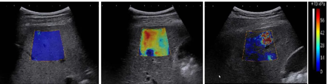
The quality of the acquired shear wave elasticity maps was very variable from one exam to the other as illustrated in Fig. 1 which shows different elasticity maps that can be encountered: high quality data and homogeneous SWE with complete filling of the elasticity map and low spatial variation (Fig. 1a), heterogeneous data with complete filling of the elasticity map but high spatial variation (Fig. 1b) and low quality data with a partial filling of the elasticity map (Fig. 1c).

Exploitable SWE measurements could not be obtained in three patients (n=3/31) because of patient obesity or anatomical inaccessibility, which hindered the propagation of shear waves. This showed as no or very little filling of the elasticity map. For these three cases, the percentage of unfilling of the elasticity map was greater than 60% and the candidate patient was excluded from the study. Acquisition failures occurred in three patients (n=3/31). There were 28 patients in the remaining population (n=28/31) included in the statistical analysis.

b) Data quality indexes

Across the whole set of clips, the values of the temporal variability (TV) parameter ranged from 0.05 to 3.4 kPa, the percentage of unfilling across the clip (PNF) ranged from 0 to 49% and the spatial variation ranged from 0.2 to 24.8 kPa. Table 1 summarizes the min, max, mean and median values of each quality parameter. From the distribution of these values, a threshold value was defined for each parameter in order to separate high from low quality clips: 1 kPa for TV, 10% for PNF and 2 kPa for SV. The thresholds were chosen so that about one fourth of the clips be classified in the low quality category.

The correlations between each parameter (TV, PNF and SV) and the expert measured elasticity (Eexp)

were assessed (Fig. 2). The temporal variability (TV) and the elasticity were correlated with a Pearsons’ correlation coefficient r=0.44 (p <0.001). There was no significant correlation between the percentage of non filling (PNF) and the elasticity (r=0.062). The spatial variability (SV) was the parameter the most correlated with the elasticity with a Pearsons’ correlation coefficient r=0.67 (p <0.001).

8 c) SWE acquisition intra-observer accuracy

To compute the Exp acquisition variability, all the combinations of clips for a same patient were analyzed. We found a mean variability of acquisition between clips 𝑉_𝑎 of 22% corresponding to an ICC of 0.855. Since the clips that were compared had different quality parameters, the mean values of

TV, SV and PNF of the different clips of a given patient i were computed (TVi, SVi and PNFi) in order

to get one value per patient for each parameter. Exams characterized by either a PNFi or a TVi above

the criteria thresholds were classified as low grade exams (LGi) while exams meeting the PNFi and

TVi criteria were classified as high grade exams (HGi). About one third of the clips (NC=27) belonging

to 9 patients were classified as LGi and showed an acquisition variability of 32.5%. The remaining

population (NC=57 corresponding to 19 patients) had a variability of 17%. The acquisition variability for different groups of patients separated according to the quality indexes (TVi, SVi and PNFi) is

summarized in Table 2.

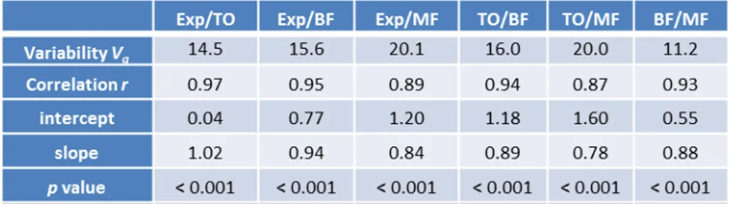
d) SWE quantification inter-observer variability

The mean elasticity values of the acquired elasticity maps were computed using the different methods described in sub-section (c) of the Material and Methods section. For each clip, the mean elasticity measured by the expert was compared to that measured by the trained operator (TO) and the two automatic methods (BF and MF). The plot of the mean elasticity values measured by the expert (abscissa) versus the TO, BF and MF methods (Fig. 3a) for the whole population (N=84 clips) shows that the correlation is higher for clips that have low elasticity values than high ones. This is also highlighted by the Bland-Altman plot of differences in SWE measurements performed by the different operators (Fig. 3b) which shows that absolute differences are generally smaller for low than for high elasticity values. Correlations of 0.97, 0.95 and 0.89 (p < 0.001) were found between the measurements of the expert and the TO, BF and MF methods respectively (Table 3). Characteristics of the linear fittings (intercept and slope) are also shown in Table 3. The percentages of variability between the measurements of the different observers for the general population ranged between 11.2 and 20.1 % (table 3). The variability between the two manual methods was 14.5% and the variability

9

between the two automatic methods was 11.2%. The variability between a manual and an automatic method ranged from 15.6% to 20.1% (17.9% in average). The BF method presented a variability with Exp and TO of 15.6% and 16% and the MF method of 20.1% and 20% respectively.

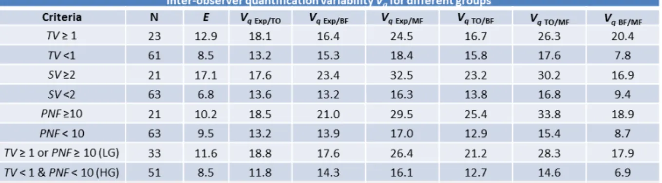
The variability between the measurements of the expert and those of the different observers for sub-groups of clips defined according to the thresholds of the different individual and combined quality parameters (TV, PNF and SV) was also computed (table 4). The variability between the two manual methods was 18.1% for unstable clips (TV≥1) and 13.2% for stable clips (TV<1). The variability between the two automatic methods was 20.4% and 7.8% for unstable and stable clips respectively. The average variability for all pairs of methods was also 20.4% for unstable clips and 14.7% for stable clips. The average variability for all pairs of methods was 13.9% for spatially homogeneous clips (SV<2) and 24.0% for heterogeneous clips with SV≥2. The average variability for all pairs of methods was 13.5% for highly filled elasticity maps (PNF<10) and 24.5% for PNF≥10. Clips presenting either a PNF or a TV above the criteria thresholds were classified as low grade clips (LG). This concerned 33 clips which in average showed an inter-observer quantification variability ranging from 17.6% to 28.3% for the different pairs of observer comparisons as summarized in Table 4. The 33 LG clips belonged to 16 different patients amongst which 5 patients had all three clips classified as LG. The remaining 51 clips met the PNF and TV criteria and were classified as high grade clips (HG). They had an inter-observer quantification variability ranging from 6.9% to 16.1% (Table 4). The mean elasticity of the population with low grade exams was about 30% higher than that of the sub-population with high grade exams (11.6 kPa in average for LG and 8.5 kPa for HG).

Discussion and conclusion

The acquisition and quantification accuracies of SWE estimates of liver were assessed in a population of patients with various hepatic pathologies. The acquisition accuracy which depends on the positioning of the probe and shear window was assessed by comparing elasticity estimates obtained on consecutive clips acquired by the same expert on a same patient after repositioning the probe (intra-observer inter-clip variability). The quantification accuracy depends only on the choice of the

10

measurement frame and area and was assessed by comparing the expert measurement with the measurement performed by a trained operator and 2 automatic methods on a same registered video clip (inter-observer intra-clip variability).

Previous reproducibility studies of SWE measurements in the liver reported by Ferraioli (Ferraioli et al., 2012b) showed ICC values of 0.95 and 0.93 for intra-observer SWE measurements performed the same day and 0.84 and 0.65 for measurements performed on different days by the expert and novice operators respectively. In (Hudson et al., 2013), the authors found SWE to be repeatable and reliable (ICC=0.92-0.87). In order to confront our findings to these previous studies, we evaluated the intra-observer ICC and found an agreement for same day assessments of 0.85 which is slightly below the agreements observed in (Ferraioli et al., 2012b)(Hudson et al., 2013). It is important to note that these previous studies only concerned healthy subjects, with homogeneous and soft livers and generally good quality elasticity maps. We had previously observed that soft livers provide highly reproducible measurements (Labit et al., 2013). This was confirmed by the results of this study.

In order to provide the radiologist with an estimation of the reliability and accuracy of a given SWE measurement in clinical practice, we attempted to evaluate the variability of SWE measurements according to parameters depending on the data quality instead of the liver elasticity. Data quality parameters based on temporal stability (TV- Temporal Variability parameter) and propagation of shear waves (PNF- Percentage of Non Filling parameter) as well as a spatial homogeneity parameter (reflected by the Spatial Variation SV) were defined for that purpose and computed in all the clips. In order to evaluate whether these parameters reflected not only the pathology but also the quality of the data, correlations between these parameters and the measured elasticity were computed. The PNF parameter of the clip was found to be insignificantly correlated to the elasticity value measured in the clip. This is not surprising as the PNF should more likely be related to subcutaneous fat thickness than to liver stiffness. The spatial variability parameter was found to be correlated to the elasticity which was expected as the higher the elasticity, the higher its fluctuations. The temporal variability was moderately correlated with the elasticity. In order to provide an automatic estimation of each clip or exam quality (high or low grade), a criterion combining the TV and PNF parameters was defined. The

11

SV parameter was excluded from the criterion as it is related to the standard deviation measurement

which is already displayed in the system Q-box and which reflects the variability of the measurement due to the liver heterogeneity more than that due to the data quality (artifacts).

The intra-observer expert acquisition variability Va was higher than the inter-observer variability

between all quantification methods. This is not surprising as some discrepancies arise from the positioning of the probe. The proposed qualitative data related criterion (high grade or low grade) was shown to be related to the acquisition variability. The acquisition variability was almost twice higher for exams classified as low grade than for high grade exams. The acquisition variability for high quality data is in agreement with the constructor precision of 15%.

The average correlation between the different quantification methods was excellent (ranging from 0.87 to 0.98). The agreement between methods is much higher for low elasticity values than for high ones as shown on the Bland-Altman plot in Fig.3 where the points are less scattered in the low elasticity range than in the high one. Concerning the quantification accuracy, the variability between the two manual methods was lower than the variability between a manual and an automatic method. The BF method presented a lower variability with the manual methods than the MF method. Moreover, the variability between the two automatic methods was almost three times higher for unstable clips (TV≥1) than for stable clips (TV<1). This was expected as the mean frame is only representative of the clip when the temporal stability is high. When splitting the population according to the PNF criteria, the variability for clips that have a low PNF is less than 17% between all quantification methods while it is measurement method dependent when the PNF is higher with a range of 18.5 to 33.8 % between all quantification methods. This indicates that the choice of the area of measurement is crucial when the clips are of poor quality. This also suggests that the mean elasticity is not very pertinent for poor quality clips as it very much depends on where the measurement is performed. The SV criteria also allows to split the population of clips between the ones that have reproducible measurements (13.9% variability in average), and the ones that are less reproducible (24.0% variability in average). This parameter is also highly related to the elasticity as stated above with a mean elasticity for clips with

12

As for the acquisition variability, exams classified as low grade quality have a significantly higher quantification related variability (17.6 to 28.3% for all comparisons of quantification methods) than high grade exams (quantification related variability of 6.9 to 16.1%). This quality index provides a confidence grading and allows deducing whether elasticity estimates can be considered accurate and reliable or not.

This study demonstrated that elasticity values obtained with the SWE technique are accurate for high quality exams according to the defined quality criteria, and must be interpreted cautiously for low quality exams. This quality assessment does not provide a marker totally unrelated to the elasticity itself, the average elasticity of low quality exams being about 30% higher than that of high quality exams.

The goal of this study was to evaluate the accuracy of SWE measurements in diseased livers and not to state on the capability of SWE to discriminate between different stages of fibrosis. A correlation with pathology would have to be performed for that purpose. A recommendation from this study is to acquire SWE clips because they make it possible to perform additional quantifications on a more stable frame if necessary. They also allow assessing the quality of the data. If the quality is low, additional clips can be acquired which might be of better quality. Amongst the 31 patients initially included in the study, acquisition failures due to narrow inter-costal space or obesity occurred in three patients (10%) and there were five patients (16%) who had all their clips classified as low grade. The remaining 23 patients (74%) had at least one high grade clip making it possible to confidently assess the liver elasticity for most patients.

Our conclusion about the importance of taking into account the quality of the data could certainly be extended to SWE studies concerning other organs. These quality criteria could easily be implemented in a commercial machine in order to provide an estimation of the accuracy of the measurement.

Appendix

13 𝑇𝑉 =_𝑛 4

𝑓.∆𝑥.∆𝑦∑ 𝐸𝑥,𝑦

𝑓

𝑓,𝑥,𝑦 (1)

where nf represents the number of frames in the clip, ∆𝑥 and ∆𝑦 are the lateral and axial sizes of the

insonation window and 𝐸_𝑥,𝑦𝑓 represents the elasticity of pixel px,y (𝑥 = [∆𝑥/4,3∆𝑥/4 ], 𝑦 = [∆𝑦/4,3∆𝑦/4 ]) in

the frame f (𝑓 = [1, 𝑛𝑓 ]).

A2) The percentage of non-filling parameter PNF was expressed as:

𝑃𝑃𝑃 =_{∆𝑥.∆𝑦}1 (𝑛𝑛𝑛𝑛𝑛𝑛 𝑝𝑝𝑥𝑛𝑝𝑝 / 𝐸𝑥,𝑦𝑓∗ = 0) (2)

where f* represents the best frame selected by the AAE algorithm

A3) The spatial variation parameter SV was expressed as:

𝑆𝑉 = �∑ ∑ �𝐸𝑥,𝑦𝑓∗−𝐸�𝑓∗� 2 ∆𝑦 𝑦=1 ∆𝑥 𝑥=1 (∆𝑥.∆𝑦−1) (3)

where 𝐸�𝑓∗ is the mean elasticity value in the frame f* . A4) The acquisition variability was defined as:

𝑉𝑎=_𝑁𝑁1 ∑ ∑ 2�𝐸𝑒𝑥𝑒 𝑖 _{(𝑗)−𝐸𝑒𝑥𝑒}𝑖 _�𝑗′_�� 𝐸𝑒𝑥𝑒𝑖 (𝑗)+𝐸𝑒𝑥𝑒𝑖 (𝑗′) 𝑁𝑖 𝑗,𝑗′₌₁ (𝑗′_≠𝑗) 𝑃 𝑖=1 (4)

where 𝐸_𝑒𝑥𝑒𝑖 (𝑗)and 𝐸_𝑒𝑥𝑒𝑖 (𝑗′) represent the mean elasticity values measured by Exp in two different clips (𝑗 and 𝑗′) of patient 𝑝, 𝑃 represents the number of patients, NC the total number of combinations of clips and 𝐶_𝑖 the number of combinations of clips corresponding to patient 𝑝.

A5) The quantification inter-observer relative variability was defined as:

𝑉𝑞=_𝑁1∑ ∑ 2�𝐸𝑒𝑥𝑒 𝑖 _{(𝑗)−𝐸} 𝑜𝑜𝑜𝑖 (𝑗)� 𝐸𝑒𝑥𝑒𝑖 (𝑗)+𝐸𝑜𝑜𝑜𝑖 (𝑗) 𝑛𝑖 𝑗 𝑃 𝑖=1 (5)

where 𝐸_𝑜𝑜𝑜𝑖 (𝑗) represents the mean elasticity value measured in the clip 𝑗 of patient 𝑝 by an operator different than the expert (𝑜𝑛𝑝 = {TO, BF, MF}), N the total number of clips and 𝑛_𝑖 the number of clips corresponding to patient 𝑝.

14

Acknowledgments

The authors wish to thank the French Cancer Association ARC (Association pour la Recherche sur le Cancer) for their generous funding (grant number SFI20111203653).

References

Afdhal, N.H., Nunes, D., 2004. Evaluation of liver fibrosis: a concise review. Am. J. Gastroenterol. 99, 1160–74.

Bedossa, P., Bioulac-Sage, P., Callard, P., Chevallier, M., Degott, C., Deugniar, Y., Fabro, M., Reynes, M., Voigt, J.J., Zafrani, E.S., Poynard, T., Babany, G., 1994. Intraobserver and interobserver variations in liver biopsy interpretation in patients with chronic hepatitis C. Hepatology 20, 15–20.

Bensamoun, S.F., Wang, L., Robert, L., Charleux, F., Latrive, J.-P., Ho Ba Tho, M.-C., 2008. Measurement of liver stiffness with two imaging techniques: magnetic resonance elastography and ultrasound elastometry. J. Magn. Reson. Imaging 28, 1287–92.

Bercoff, J., Tanter, M., Fink, M., 2004. Supersonic shear imaging: a new technique for soft tissue elasticity mapping. IEEE Trans Ultrason Ferroelectr Freq Control 51, 396–409.

Castera, L., 2009. Transient elastography and other noninvasive tests to assess hepatic fibrosis in patients with viral hepatitis. J. Viral Hepat. 16, 300–14.

Cosgrove, D.O., Berg, W. a, Doré, C.J., Skyba, D.M., Henry, J.-P., Gay, J., Cohen-Bacrie, C., 2012. Shear wave elastography for breast masses is highly reproducible. Eur. Radiol. 22, 1023–32.

Fahey, B.J., Nelson, R.C., Bradway, D.P., Hsu, S.J., Dumont, D.M., Trahey, G.E., 2008. In vivo visualization of abdominal malignancies with acoustic radiation force elastography. Phys. Med. Biol. 53, 279–293.

15

Ferraioli, G., Tinelli, C., Zicchetti, M., Above, E., Poma, G., Di Gregorio, M., Filice, C., 2012b. Reproducibility of real-time shear wave elastography in the evaluation of liver elasticity. Eur. J. Radiol. 81, 3102–6.

Ferraioli, G., Tinelli, C., Dal Bello, B., Zicchetti, M., Filice, G., Filice, C., 2012a. Accuracy of real-time shear wave elastography for assessing liver fibrosis in chronic hepatitis C: a pilot study. Hepatology 56, 2125–33.

Fraquelli, M., Rigamonti, C., Casazza, G., Conte, D., Donato, M.F., Ronchi, G., Colombo, M., 2007. Reproducibility of transient elastography in the evaluation of liver fibrosis in patients with chronic liver disease. Gut 56, 968–73.

Hudson, J.M., Milot, L., Parry, C., Williams, R., Burns, P.N., 2013. Inter- and intra-operator reliability and repeatability of shear wave elastography in the liver: a study in healthy volunteers. Ultrasound Med Biol 39, 950–955.

Klatt, D., Asbach, P., Rump, J., Papazoglou, S., Somasundaram, R., Modrow, J., Braun, J., Sack, I., 2006. In vivo determination of hepatic stiffness using steady-state free precession magnetic resonance elastography. Invest. Radiol. 41, 841–848.

Labit, M., Pellot-Barakat, C., Lefort, M., Frouin, F., Lucidarme, O., 2013. Reproducibility of liver elasticity assessed by shear wave elastography. Eur. Congr. Rad, C-1025, Vienne.

Muller, M., Gennisson, J.-L., Deffieux, T., Tanter, M., Fink, M., 2009. Quantitative viscoelasticity mapping of human liver using supersonic shear imaging: preliminary in vivo feasibility study. Ultrasound Med Biol 35, 219–229.

Palmeri, M.L., Wang, M.H., Dahl, J.J., Frinkley, K.D., Nightingale, K.R., 2008. Quantifying hepatic shear modulus in vivo using acoustic radiation force. Ultrasound Med. Biol. 34, 546–58.

16

Poynard, T., Munteanu, M., Luckina, E., Perazzo, H., Ngo, Y., Royer, L., Fedchuk, L., Sattonnet, F., Pais, R., Lebray, P., Rudler, M., Thabut, D., Ratziu, V., 2013. Liver fibrosis evaluation using real-time shear wave elastography: applicability and diagnostic performance using methods without a gold standard. J Hepatol 58, 928–935.

Sandrin, L., Fourquet, B., Hasquenoph, J.-M., Yon, S., Fournier, C., Mal, F., Christidis, C., Ziol, M., Poulet, B., Kazemi, F., Beaugrand, M., Palau, R., 2003. Transient elastography: a new noninvasive method for assessment of hepatic fibrosis. Ultrasound Med. Biol. 29, 1705–1713.

Tanter, M., Bercoff, J., Athanasiou, A., Deffieux, T., Gennisson, J.-L., Montaldo, G., Muller, M., Tardivon, A., Fink, M., 2008. Quantitative assessment of breast lesion viscoelasticity: initial clinical results using supersonic shear imaging. Ultrasound Med. Biol. 34, 1373–1386.

17

Tables

Table 1: Description and distribution of the quality parameters values; nf represents the number of frames in the

investigated clip, Thr represents the threshold value of the parameter, r and p represent the Pearson correlation with the elasticity measurement and its significance.

Table 2: Percentage of variability between elasticity measurements of different clips of the same patient performed by the expert radiologist. The mean variability was computed for different groups of exams separated according to the individual quality parameters of the exam (TVi, SVi and PNFi) as well as for Low Grade (LGi)

and High Grade (HGi) exams. NC represents the total number of combinations of clips and P the number of

patients in each category.

Table 3: Percentages of variability and coefficient of correlation between the expert (Exp) and observer (TO, BF and MF) measurements over the whole population.

18

Table 4: Variability between the expert and observer (TO, BF and MF) measurements according to quality criteria (TV: Temporal Variability, SV: Spatial Variation, PNF: Percentage of Non Filled pixels). The last 2 rows correspond to low quality clips (TV or PNF criteria not met) and high quality clips (TV and PNF criteria met).

19

Figure Legends

Fig. 1: SWE images of right livers accessed intercostally. a) Low spatial variation (SV=0.78) with high quality elasticity map (PNF=0%); b) Heterogeneous spatial distribution (SV=4.11) with high filling (PNF =0%), c) Heterogeneous spatial distribution (SV=7.88) with poor filling (PNF=49%).

Fig. 2: Quality parameter as a function of the estimated elasticity for the 84 clips. Pearson’s correlations of 0.40, 0.06 and 0.69 are found between the elasticity and TV, PNF and SV respectively.

Fig. 3: a) SWE estimates of the N clips (N=84 corresponding to P=28 patients) using the Trained Operator (TO), Best Frame (BF) and Mean Frame (MF) measurement methods as function the Expert measurement (Exp), b) Bland–Altman plot of differences in ratings performed by the expert and the three other operators. The blue,

20

red and green solid lines represent the mean of difference of ratings. The dashed lines define the limits of agreement.