Quantifying effectiveness of cathodic protection in water mains: theory

Publisher’s version / Version de l'éditeur:

Journal of Infrastructure Systems, 10, June 2, pp. 43-51, 2004-06-01

READ THESE TERMS AND CONDITIONS CAREFULLY BEFORE USING THIS WEBSITE. https://nrc-publications.canada.ca/eng/copyright

Vous avez des questions? Nous pouvons vous aider. Pour communiquer directement avec un auteur, consultez la

première page de la revue dans laquelle son article a été publié afin de trouver ses coordonnées. Si vous n’arrivez pas à les repérer, communiquez avec nous à PublicationsArchive-ArchivesPublications@nrc-cnrc.gc.ca.

Questions? Contact the NRC Publications Archive team at

PublicationsArchive-ArchivesPublications@nrc-cnrc.gc.ca. If you wish to email the authors directly, please see the first page of the publication for their contact information.

NRC Publications Archive

Archives des publications du CNRC

This publication could be one of several versions: author’s original, accepted manuscript or the publisher’s version. / La version de cette publication peut être l’une des suivantes : la version prépublication de l’auteur, la version acceptée du manuscrit ou la version de l’éditeur.

For the publisher’s version, please access the DOI link below./ Pour consulter la version de l’éditeur, utilisez le lien DOI ci-dessous.

https://doi.org/10.1061/(ASCE)1076-0342(2004)10:2(43)

Access and use of this website and the material on it are subject to the Terms and Conditions set forth at

Quantifying effectiveness of cathodic protection in water mains: theory

Kleiner, Y.; Rajani, B. B.

https://publications-cnrc.canada.ca/fra/droits

L’accès à ce site Web et l’utilisation de son contenu sont assujettis aux conditions présentées dans le site LISEZ CES CONDITIONS ATTENTIVEMENT AVANT D’UTILISER CE SITE WEB.

NRC Publications Record / Notice d'Archives des publications de CNRC:

https://nrc-publications.canada.ca/eng/view/object/?id=eb750ae5-daec-4d2b-ace9-ca68af258eb2 https://publications-cnrc.canada.ca/fra/voir/objet/?id=eb750ae5-daec-4d2b-ace9-ca68af258eb2

Quantifying effectiveness of cathodic protection in water mains: theory

Kleiner, Y.; Rajani, B.

NRCC-38457

A version of this document is published in / Une version de ce document se trouve dans : Journal of Infrastructure Systems, v. 10, no. 2, June 2004, pp. 43-51

QUANTIFYING EFFECTIVENESS OF CATHODIC

PROTECTION IN WATER MAINS: THEORY

Yehuda Kleiner and Balvant Rajani

Institute for Research in Construction, National Research Council Canada, Ottawa, Ontario Canada K1A 0R6

Tel: (613)-993-3805, fax: (613)-954-5984 E-mail: Yehuda.Kleiner@nrc.ca

QUANTIFYING EFFECTIVENESS OF CATHODIC

PROTECTION IN WATER MAINS: THEORY

Yehuda Kleiner and Balvant Rajani

Abstract: Cathodic protection is a viable measure to extend the residual life of water mains and thus defer capital investments in their rehabilitation and renewal. The

effectiveness of cathodic protection varies with the unique set of conditions under which it is applied and it is difficult to confirm or validate whether its application can be considered successful. Therefore, the reported success histories have been largely anecdotal and most often based on the reduction of water main breaks using cathodic protection.

This paper describes methodologies and associated models to quantify and assess the performance of cathodic protection programs implemented by water utilities. The effectiveness of cathodic protection programs applied under various conditions can be determined and weighed against their costs in order to maximise the benefit from their implementation. These proposed methodologies and models should assist water utilities to optimise the implementation and scheduling of future cathodic protection programs. A companion paper “Quantifying Effectiveness of Cathodic Protection in Water Mains: Case studies” describes the application of proposed models to assess the impact of cathodic protection programs.

Key words: water main deterioration, hot spot, retrofit, cathodic protection, water main renewal, life-cycle costs.

INTRODUCTION

Communities depend on a safe and reliable delivery of drinking water for domestic, industrial and fire fighting purposes. The water distribution network is the most

expensive component in a typical water supply system and it often involves up to 80% of its total expenditure (Clark and Gillian, 1977). Kirmeyer et al. (1994) estimated that in 1992 in the United States, more than two thirds of all existing water pipes were metallic (about 48% cast iron and 19% ductile iron), about 15% were asbestos-cement and the remaining 18% were plastic, concrete and others. A survey encompassing 21 Canadian cities (about 11% of the population of Canada), conducted by Rajani and McDonald (1995), revealed a similar distribution of pipe material types.

In most North American cities, metallic water mains deteriorate as a consequence of aggressive soil conditions, use of dissimilar metals, stray electric currents due to electrical grounding or other sources of currents, etc. These conditions encourage external corrosion pits in ductile iron or formation of graphitised zones in cast iron. Under extreme conditions, corrosion can impact pipe integrity as early as 5 years after installation. Cathodic protection (CP) of cast and ductile iron mains is a mitigative measure that has been implemented in many cities in recent years to reduce premature breaks and leaks in the water distribution network.

Cathodic protection can be defined as “…the reduction or elimination of corrosion by making the metal a cathode by means of an impressed direct current or attachment to a sacrificial anode (usually magnesium, aluminium or zinc)” (NACE, 1984). Ideally, a cathodic protection system should distribute protective current evenly over the entire pipe surface. However, the geometry of CP (discrete anodes protecting a continuous pipe resulting in varying distances between the anode and any point along the pipe) as well as variability in soil composition and presence of shielding structures, will result in variable attenuation of current and its uneven distribution along the pipe.

The difficulty in quantifying the effectiveness of CP is due to the fact that this

effectiveness can vary with the unique set of conditions under which CP is applied. If the effectiveness of CP could be determined and weighed against its costs then its benefits

could be maximised, making CP a viable measure for extending the residual life of water mains and thus defer capital investments in their rehabilitation and renewal.

In this paper, models and methods to quantify and assess the performance of cathodic protection programs implemented by water utilities are described. These methods should assist water utilities to optimise the implementation and scheduling of future cathodic protection programs.

The remainder of this paper is organised as follows. In the next section the

time-dependent breakage-forecasting model is briefly described. This multicovariate model is the platform within which the effectiveness of cathodic protection is quantified, based on historical breakage patterns before and after CP implementation. The third section describes the model to predict breakage rates in water mains cathodically protected using a hotspot strategy, as well as a method to assess its costs and benefits as a function of the time of implementation. The fourth section describes a model for predicting breakage rates in water mains that are retrofitted by cathodic protection anodes as well as a method to assess costs and benefits in order to select the best implementation strategy. The fifth section briefly discusses some theoretical issues that are relevant to the methods

presented in sections three and four. Summary and conclusions are provided in the final section. The examples used in this paper are solely to illustrate the behaviour and sensitivity of the models. A companion paper “Quantifying Effectiveness of Cathodic Protection in Water Mains: Case studies” (Rajani, Kleiner and McDonald, 2003) provides in-depth descriptions of several case studies that demonstrate the application of the models using the WARP (Water Mains Renewal Planner) software program.

TIME-DEPENDENT MULTICOVARIATE WATER MAIN BREAK

PREDICTION MODEL

Shamir and Howard (1979) were the first to suggest that an exponential function could be used to represent the increase in water main breakage rates with pipe age. They proposed a two-parameter (single variate – age) exponential function, which was subsequently used by others (e.g, Walski and Pelliccia, 1982; Clark et al., 1982; Kleiner et al., 1998; Kleiner and Rajani, 1999). Kleiner and Rajani (2000, 2002) proposed a

generalised form of the exponential model that included multiple covariates which can be time-dependent. t x a t N x e x N( )= ( t₀) ⋅ (1)

where t = time elapsed from year of reference to, xt = row vector of time-dependent

covariates prevailing at time t, N(xt) = number of breaks at time t (resulting from xt), a=

column vector of parameters corresponding to covariates x, and

0

t

x = vector of baseline x

values at year of reference to.

Time-dependent covariates (or “explanatory variables”) can be pipe age, temperature, soil moisture, number of effective CP anodes, etc. Parameters N

( )

time-dependent covariates could be extended to other break increase models such as the power model (e.g., Constantine and Darroch, 1993).

HOTSPOT CATHODIC PROTECTION (HS CP)

Hotspot cathodic protection is the practice of opportunistically installing a protective (sacrificial) anode at the location of a pipe repair. These anodes are typically installed without any monitoring and stay in the ground until total depletion, usually without replacement. The following is assumed in the development of a model to assess the effect of HS CP on the breakage rate of a (relatively homogeneous) group of pipes: • A hotspot anode has an effective life of tLF years in the ground.

• A hotspot anode provides full protection after a time lag of tLG from time of

installation.

• When a HS CP program commences at year THS for a given group of pipes, every

break repair reported from year t onwards includes a hotspot anode. This anode provides active protection starting at time t + tLG and ending at time t + tLF.

• The exact location of a break (and a HS anode) along a pipe is assumed to be random. It is also assumed that a higher breakage frequency is likely in pipe segments that are more deteriorated than other segments. The effectiveness of the active HS anodes (in terms of reducing breakage frequency) is expected to be higher at the beginning of the HS CP program, because many of these anodes will be placed in the more deteriorated parts of the network. However, as new anodes are continually added, some are likely to be placed close to existing active anodes. Consequently, as the number of breaks increase over time, additional placement of anodes is likely to have a diminishing impact and reflect a local “crowding effect”. This effect is represented in the proposed model by an effectiveness factor fe ,

which has been empirically established to vary between 0.7 and 2.

• For the time-dependent, multivariate analysis of breakage history, the HS CP covariate is taken as the number of active anodes per unit length of pipe in a given group of water mains, multiplied by the effectiveness factor fe. The HS CP covariate

is thus dependent both on the total length of the water mains at year t and the number of breaks in previous years.

The number of active HS anodes at year t, Atac is expressed by,

∑

∑

and the actual HS CP covariate is given by,

e t t ac HSCP t f L A X _      = (3)

where Lt is the total length of water mains in the group at year t, and fe is an effectiveness

factor given by ) exp( 3 . 1 7 . 0 t t ac e L A k f = + − (4)

Several functions were considered before arriving at the proposed function in (4). An examination of (4) indicates that the effectiveness factor is close to 2 when the number of active HS anodes is small. The effectiveness factor, fe, decreases and approaches the

value of 0.7 as the number of active anodes increases. The rate of this decrease is dependent on the magnitude of k.

As mentioned earlier, parameters a are found by regression or ML method, where covariate Atac and parameter k are computed from the number of observed historical

breaks. Once regression parameters are found, the impact of HS CP on future breakage rate can be determined and life-cycle cost analysis can be performed.

The following example considers only age and HS CP as covariates affecting pipe breakage rate. It illustrates the dependence of the breakage rate on the number of active HS anodes. The life of anodes, tLF , is assumed to be 15 years and the time lag, tLG, is

assumed to be 1 year.

The total number of breaks at pipe age t is given by HSCP t X a t a HSCP t HSCP t N t X e X t N 1 2 0 ) , ( ) , ( = ₀ + (5)

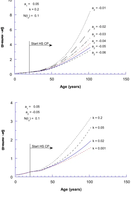
where a1 is the ageing parameter and a2 is the HS CP parameter. Figure 1 illustrates the

forecasted breakage rates given various combinations of a1 and a2 and effectiveness

factor parameter k. Hotspot cathodic protection is assumed to start at a pipe age of 20 years. The year of reference to is assumed to be the year of installation (age zero).

It can be seen in Figure 1 that the more negative the HS CP parameter a2 gets, the more

effective HS CP strategy is in reducing breakage rate. The impact of HS CP on the breakage rate of pipes is small in the early life of the pipe and the breakage rates increase becomes more significant as the pipe ages. This response is expected because the number of anodes is directly related to the number of previous pipe breaks.

The effectiveness factor, fe, might be expected to have a lower value of parameter k in

high resistivity soils, where the effect of a single anode is more localised, and overcrowding is less likely. However, higher resistivity soils are also less likely to promote corrosion, so breakage rates are likely to be relatively low and the effectiveness factor may not have much impact.

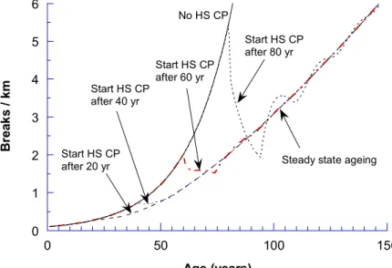
Figure 2 demonstrates the effect of commencing a HS CP program at various stages in the life of a pipe. For illustrative purposes, parameters a1 and a2 were intentionally

assigned high values to accentuate the effect.

When the HS CP program commences relatively early in the life of the pipe, the breakage rate remains relatively low and converges early to a steady state rate. On the other hand, the breakage rate drops rapidly when the HS CP program commences relatively late in the life of the pipe1. After several years the breakage rate converges to the same steady state breakage rate as that of the earlier protected pipes. This pronounced drop in breakage rate occurs because the CP program starts when the breakage rate is high, and consequently many HS anodes are placed in a relatively short period. This large number of anodes creates a significant drop in breakage rate. Thus, if the HS CP programs starts late in the life of the pipe at year t, the subsequent year t+1 will see a relatively large drop in breakage rate because a large number of anodes were placed in year t. The subsequent year t+2 will see a further drop in breakage rate, but this drop will be smaller than that in year t+1, because fewer anodes were placed in the preceding year. Subsequent years will see smaller and smaller declines in breakage rate. As the first anodes start to expire, the breakage rate will start increasing, triggering a higher rate of anode placement. The net effect is a breakage rate that oscillates until it converges to a steady state rate. The degree of oscillation and the speed of convergence depend on the pipe breakage rate at program commencement, on HS CP parameter and on the effectiveness factor.

Life-Cycle Cost of Pipes with Hotspot Cathodic Protection (HS CP)

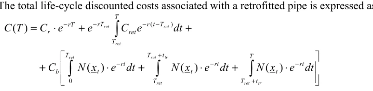
The total discounted life costing of a pipe from the present time (time of decision making) until it is replaced at time T is expressed in the following,

∫

Note that the terms “early” and “late” in this context refer to the state of deterioration of the pipe rather than its chronological age.

where Cr = cost to replace a unit length of pipe ($/km), r = equivalent continuous

discount rate, T = the year at which the pipe is replaced (time elapsed from the present),

Cb = cost of a single breakage, including direct, indirect and social costs, CHS = cost of a

hotspot anode, N(xt) = number of breaks per unit length as defined in (1) (km-1 year-1),

t = integration variable.

The first term on the right hand side of equation (6) is the discounted cost of pipe replacement, while the expression under the integral is the total discounted cost of all breaks (including HS CP anodes) from the present time (year zero) until the pipe is replaced.

Impact of HS CP on Cost of Breakage Repair

The impact of the the HS CP in the proposed model on the cost of pipe repair is

demonstrated with examples, in which relevant costs and parameters were assumed to be:

Cb = $5,000/break, CHS = $250/anode, Cr = $300,000/km of pipe replaced,

tLF = 15 years (anode life), tLG = 1 year (time lag), r = 3% (discount rate). Figure 3 shows

the total cumulative (discounted) cost of breaks and how it varies depending on the time at which HS CP commences. Note that the present time (year zero) in this example is taken as the year of installation, so that costs include the total life cycle.

Figure 3 shows that there is little cost saving when HS CP is implemented very early in the life of a pipe. This is expected because at an early deterioration stage the number of breaks is relatively small and the number of HS anodes will thus be small, resulting in a very small difference in breakage rates with or without HS CP. As the pipe ages and deteriorates further, the cost savings in implementing HS CP become increasingly more significant. It can also be seen that the differences in costs are approximately constant (e.g., the cost curves of HS CP commencing at 40, 60 and 80 years are nearly parallel). This model response is also expected, as described in Figure 2, given that once HS CP is implemented, breakage rate approaches the same steady state regardless of when it was implemented.

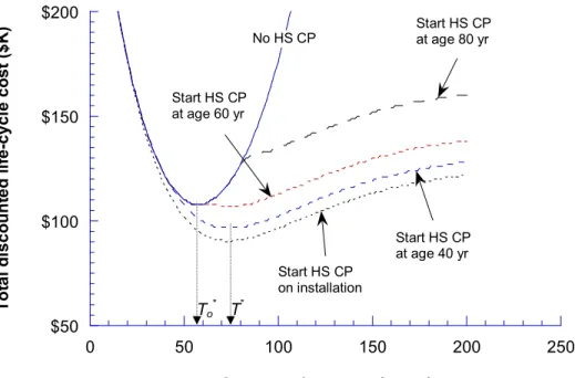
Total Costs and Optimal Replacement Timing

The cost of breakage repair increases as the time of replacement is delayed because of pipe deterioration (term under the integral in equation (6)) but at the same time the deferred cost of replacement decreases because of discounting (first term on the right hand side of equation (6)). The total cost curve, as is shown in Figure 4, is typically convex, with a minimum cost denoting the optimal time for replacement T*. This optimal replacement time T* could be viewed as the point in time at which the economic life of the pipe ends (Kleiner and Rajani, 1999). Strictly speaking, the replacement (new) pipe will also have a breakage rate that increases with age and will incur an additional

maintenance cost. This cost should also be considered in finding T*. This issue is further discussed subsequently.

Figure 4 illustrates that potential savings in total life-cycle cost are greater the sooner HS CP is implemented. However, there is little benefit in implementing HS CP very early in the life of a pipe because the incremental savings are very small (of course in early stages the incremental cost of HS anodes is small as well because of low breakage rate). In this example, if a pipe is eventually replaced at year 80 (point A), then its total discounted life-cycle cost if no HS protection were applied is approximately $128,000 (including repair and replacement but excluding initial installation). If HS CP is applied to this pipe at an earlier stage, say at points B or C, the total discounted life-cycle cost reduces to approximately $90,000 or $108,000, respectively.

Impact of HS CP on Pipe Replacement Timing

Under certain conditions HS CP can delay the optimal time of pipe replacement T* (Figure 5), which, as was stated earlier, could be viewed as extending the economic life of the pipe. The optimal time for replacement of an unprotected pipe is represented by To*

which, in this example is 58 years. The optimal time of replacement is not affected if HS CP commences at any year later than To*. However, the optimal time of replacement

may be delayed to year T* if HS CP commences earlier than To*. In this example T*

It is interesting to note that the magnitude of this ‘life extension’ does not depend on how early HS CP has commenced. As was demonstrated previously, the breakage rate of pipes protected by HS CP will tend to the same steady state regardless of when HS CP commences. Consequently, if HS CP is implemented sufficiently early, so as to allow the breakage rate to reach this steady state before To* , the life of the pipe will be extended by (T* - To*) years, which , in this example is

equal to 16 years. If this steady state is not reached at time To* the economic life extension

will be shorter than (T* - To*).

Effect of Future Replacement Cycles on Pipe Replacement Timing

Postponement of the time of pipe replacement not only defers the cost of installing the replacement pipe but also defers the total life-cycle cost of this replacement pipe, as well as that of the subsequent replacement pipes and so on in perpetuity. Under certain

assumptions, the present value of this infinite stream of costs can be computed (Kleiner et al. 1998) and incorporated into the calculation of the optimal time for next replacement. The main assumption that must be made in order to be able to analytically compute this infinite stream of costs is that all subsequent replacement cycles are identical in

behaviour and cost. This assumption is, of course, only a first-order approximation, as no one can predict how future pipes will perform. Kleiner et al. (1998) showed that subject to these assumptions, the future stream of costs can be evaluated and then discounted to the time of next replacement. The net effect is that an additional cost is incurred at the time of replacement. This additional cost represents the discounted total of the life-cycle costs of all subsequent replacement pipes to infinity. When evaluating alternative

strategies for a given water main, all future costs (subsequent to the next replacement) are represented by the this (same) additional cost, which accrues at the time of replacement. This cost is the same for all alternative strategies because it is assumed that for a given water main, the replacement pipe will always be the same, regardless when it is installed. In the previous example it was assumed that the cost of replacement pipe was

Cr = $300,000/km. If it is further assumed that all replacement pipes in the future will

have the same costs (installation and break repair) as the current pipe, and will have a breakage pattern parameter due to ageing, a1 = 0.025/year, then all these future

discounted costs are equivalent to approximately $53,400 that will accrue at the time of replacement. Thus at the year of replacement a cost of ($300,000 + $53,400 =) $353,400 will account for the next replacement and all subsequent life-cycle costs to infinity. If the ageing rate of future replacement pipes is assumed to be lower, say, a1 = 0.015/year, then

all the future life-cycle costs reduce to approximately $32,400.

The consideration of future life-cycle costs will typically impact the optimal times for next replacement. High future costs will tend to delay the optimal time of replacement, while low future costs will tend to expedite it. For instance, if in the example a future life-cycle cost of $53,400 was considered, then the optimal timings would defer from

To* = 58 to To* = 61 years, and from T* = 74 to T* = 80 years, for pipes without and with

HS CP, respectively. Although the impact of considering future life-cycle costs appears to be small in this example, it will have an increasing significance as the time of analysis (the present time) is closer to To*.

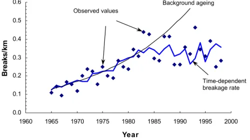
Example: HS CP Effect on Water Mains on a Southern Ontario Water Utility A group of water mains from ‘Utility A’ in Southern Ontario (Canada) was selected to illustrate the application of the proposed models. The group comprised a total of 84.4 km cast iron pipes, 100 to 300 mm in diameter, installed between 1950 and 1970, have not been retrofitted with cathodic protection, and are still in service. Utility A started an on-going HS CP program in 1979.

Figure 6 illustrates the breakage rate pattern identified for the group using equation (1), in years 1965 to 1998. The covariates used for the regression included the (mandatory) background ageing as well as freezing index (FI), rain deficit (RD), and HS CP (Kleiner and Rajani, 2000) provide a detailed explanation for the FI and RD covariates and their significance in the analysis). For the HS anodes, the life expectancy and time lag were assumed tLF = 15 years, tLG = 1 year, respectively. It should be noted that goodness of fit

statistics are not discussed in this illustrative example. These are elaborated upon in the companion paper “Quantifying Effectiveness of Cathodic Protection in Water Mains: Case studies” (Rajani, Kleiner, McDonald, 2003).

The background ageing coefficient was found to be a1 = 0.043/year (which means that if

conditions were to remain static, breakage rate would increase approximately 4.3% a year), the HS CP coefficient a2 = -0.054/year and the HS CP effectiveness parameter k =

0.05. Figure 7 shows the long-term breakage pattern expected for this group of water mains in Utility A, with and without HS CP.

Figure 8 illustrates the life-cycle cost with and without HS CP, assuming the costs of

Cb = $5,000/break for repair, CHS = $250/anode, and Cr = $300,000/km for pipe

replacement. The total discounted life-cycle cost decreases from $118,000 to

$91,000/km. As well, the optimal time for replacing these water mains is deferred from age 57 to age 87, enabling better allocation of funds. The total discounted cost of anodes from the present to age 87 is $2,540/km. Note that for simplicity life-cycle costs of future replacement pipes in this example were not considered.

RETROFIT CATHODIC PROTECTION (RETROFIT CP)

Retrofit CP refers to the practice of systematically protecting existing pipes with galvanic cathodic protection. If the existing water main is electrically discontinuous (e.g., bell and spigot with elastomeric gaskets and no bridging) then an anode is attached to each pipe segment (typically 6 m or 20’ in length)2. If the water main is electrically continuous then usually a bank of anodes in a single anode bed can protect a long stretch of pipe.

The following is assumed in the development of the model to assess the effect of retrofit CP on the breakage rate of a (relatively homogeneous) group of pipes:

• Subsequent to CP retrofitting, the pipe breakage rate reduces exponentially over a

transition period ttr. This is because the pipe is likely to have some deteriorated parts, with

imminent breakage. The CP can thus delay those breaks but not prevent them altogether.

2

There is a school of thought that claims that even without deliberate bridging water mains are electrically continuos through the electrical grounding of homes and structures that are connected to the electrical grid.

• Once the protected pipe is “purged” of these imminent breaks, a new phase begins, in which the pipe continues to age (exponential growth of breakage rate) albeit at a lower rate than before protection.

• Retrofit anodes are monitored and replaced when fully depleted, thus the slow ageing rate is maintained throughout the rest of the pipe’s life.

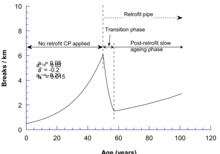
The breakage rate can then be expressed as

       ≤ + + ≤ ≤ ≤ ≤ = − − + + + ⋅ − + + ⋅ + ⋅ t t T e x t T t T e x T t t e x x N tr ret t T t a T a T a x a tr ret ret T t a T a x a ret o t a x a t tr ret tr ret t ret ret t t ; ) ( ; ) ( ; ) ( ) ( ) ( '' ' ) ( ' 1 1 1 0 0 0 t t t (7)

where Tret is the time of CP retrofit, a’ is a negative parameter depicting the reduction in

breakage rate through the transition period and a’’ is the post retrofit ageing parameter. Note that in equation (7) the row vector xt does not include pipe age, which is accounted

for in the separate terms a1t and a1Tret. Figure (9) schematically illustrates this ageing

pattern described by (7).

The validation of the proposed model for retrofitted pipes is quite challenging because only few water utilities have sufficient historical data. In addition, it is best to perform this type of analysis on relatively homogeneous groups of water mains (e.g., same type, size, vintage, etc.) to order to obtain accurate results. Furthermore, within a homogeneous group of pipes, it is preferred to trace the breakage rate of a subgroup that was retrofitted in a given year. The application of these criteria to identify relevant data ensures that a specific time-line is followed, and climatic effects can be factored out. The problem that arises is that such subgroups rarely comprise enough data to be statistically significant. A possible work-around can therefore be to pool all available breakage data so as to reflect breakage rates at years relative to the year of retrofit, rather than along an actual time line.

Three water utilities (two in Ontario and one in Alberta) were identified to have relevant data of some significance. Figure 10 shows breakage patterns before and after CP retrofit in select water main groups in these three water utilities. Case A represents all the main

breaks recorded for nearly 80 km of cast and ductile iron pipes 100 mm to 300 mm in diameter in a utility in Southern Ontario. Cases B and C illustrate the same analysis applied to CI and DI pipes 100 mm to 300 mm diameter in an Alberta utility (75 km) and an Eastern Ontario utility (36 km), respectively.

The results reflect broad averages rather than behaviour of a specific group of pipes, and climatic effects can not be factored out because no specific time-line is followed.

Nevertheless, even this aggregate analysis appears to validate the model, with adjusted coefficient of determination of 0.87, 0.89 and 0.86 for water utilities A, B and C

respectively. It can be seen that although the transition periods could be identified for the three examples, there are insufficient post-retrofit breakage data to validate the third phase of the model, namely the post-retrofit slow ageing phase.

Life-Cycle Costing of Retrofitted Pipes

The total life-cycle discounted costs associated with a retrofitted pipe is expressed as

        ⋅ + ⋅ + ⋅ + + + ⋅ =

∫

∫

∫

∫

The first term in the right hand side is the discounted cost of pipe replacement and the third term in the square brackets is the discounted cost of breakage repair in the three phases of the pipe life, depicted in equation (7). The second term in the right hand side of equation (8) is the discounted cost of retrofitting the pipe from year Tret to year T every

tLF years. Cret is the annualised cost of retrofit, expressed by

LF t retrofit ret r r C C ) 1 ( 1− + = (9)

where Cretrofit is the cost ($/km) of retrofitting a pipe.

Figure 11 illustrates an example where all replacement pipes to infinity are assumed to have the same replacement and breakage repair costs as the current pipe. The equivalent total discounted cost of all future life cycles (starting after the next replacement) is

calculated to be $42,200 (detailed calculations were done according to Kleiner et al., 1998). The following observations can be made for this example:

• The optimal age to replace the unprotected pipe is T*o = 76 years. The total discounted life-cycle cost (to infinity) if the pipe is replaced at age 76, is about $93,000/km. • The optimal age to replace the pipe if retrofitted upon installation is T* = 213years.

However, the total discounted life-cycle cost (to infinity) if the pipe is replaced at age 213, is about $110,000/km ($17,000 more than replacing unprotected pipe at year 76). The total discounted life-cycle cost increases even though the breakage rate in the protected pipe is lower because of the high present value of the up-front cost to retrofit at the time of installation. In general, however, it is expected that retrofitting pipes upon installation will be cheaper than retrofitting existing pipes because of the ease of access to the pipe. This lower cost was not considered in this example. • If the pipe is not retrofitted by age T*o , the total cost curve in the years immediately

following T*o depends on the length of the transition period ttr , on parameter a’’ and

on the cost of retrofit. For the example cited here, if the pipe is retrofitted at age 80, the total cost curve has a second minimum at T*80 = 133 years. However, if the pipe is retrofitted at age 100, then the minimum cost remains T*o. These patterns may change,

depending on specific parameters.

• Total life-cycle cost curves for the pipe retrofitted at age 40 or at age 60 are quite similar. In earlier years, the pipe retrofitted at age 40 will have a slightly higher cost because cathodic protection started earlier. However, since the breakage rate for pipe retrofitted at age 40 is lower than if it is retrofitted at age 60, after a while total costs of the former become a little lower that the latter.

• In this example the optimal strategy seems to be to retrofit the pipe at age 40 and subsequently to replace it at age T*40 = 173. The total life-cycle cost of this strategy is $69,400/km.

Because of discounting, early retrofit will have a significant impact on the discounted life-cycle costing of a pipe. The cost of retrofit depends on the cost of CP anodes, the

number of anodes per unit length of pipe and their life expectancies. Pipe size and coating and soil characteristics also influence anode density and life expectancy.

Figure 12 illustrates an example, which uses the same parameters from the previous example, except: (1) cost of retrofit Cretrofit = $20,000/km (vs. $35,000 before) and, (2)

anode life expectancy tLF = 20 years (vs. 15 years before).

It can be seen that early retrofit becomes much more attractive, compared to the previous example, because the present value of the early expenses are much smaller. Furthermore, the low cost of retrofit defers the optimal time for replacement even if retrofit is

implemented as late as age 80. The optimal strategy in this example is to retrofit the pipe at age 20, whereby the total discounted life-cycle cost is $49,200/km compared to

$69,400/km which, was the optimal cost of the previous example. Subsequently, replace the pipe at age T*20 = 202.

The magnitude of the discounting factor will also influence optimal strategy. A high discounting factor diminishes the impact of future costs and vice versa. Consequently, a lower discounting factor will tend to favour a strategy that includes an earlier retrofit. It should be noted that CP that is applied to new pipes upon installation can be viewed as a special case of retrofit, in which the time of implementation Tret = 0 and the transition

period ttr = 0. Further, applying cathodic protection upon (open cut) pipe installation is

cheaper than retrofitting an existing pipe because, (a) there is free and immediate access to the pipe, excavation and backfill costs are saved on the initial retrofit (but not on retrofit renewal), and (b) if a pipe is designed to be cathodically protected from the start, it will likely be installed with bridging to provide electrically continuous mains. In that case, anodes can be optimally spaced, as opposed to electrically discontinuous mains, where an anode should to be placed for each pipe segment.

SUMMARY AND CONCLUSIONS

The effects of hotspot cathodic protection and retrofit cathodic protection on the breakage rates of water mains were modelled within the framework of a time-dependent multi-covariate break prediction approach. As well, a process to quantify the impact of these

effects on the life-cycle costs and on the economic life of water mains was developed. The models show that the magnitude of this impact depends on the time of

implementation of the cathodic protection program.

More accurate ageing rates of water mains can be extracted from historical breakage data if consideration for the time-dependent factors such as temperatures and precipitation is allowed in the statistical analysis. The cathodic protection itself is considered as a time-dependent covariate. The hotspot CP covariate varies over time depending on the number of remaining active anodes and the length of water main. The retrofit CP is treated as a step-function that alters the breakage rate pattern of water mains after its implementation. Inferences can be made from data of other utilities with similar conditions if a water utility does not have adequate data, e.g., breakage rate before and after the

implementation of a CP program. Caution must be exercised such that inferences are applied (as much as possible) from a homogeneous group of pipes in one utility to pipes with very similar characteristics in the other utility.

A usable decision support tool in the form of a prototype computer program was developed to implement all the concepts presented here. The program enables the creation of homogeneous pipe data groups, and the automatic extraction of model parameters from data sets. It also enables to examine various planning scenarios and select the most economic strategy for water main protection/renewal. In a companion paper “Quantifying Effectiveness of Cathodic Protection in Water Mains: Case studies” (Rajani, Kleiner, and McDonald, 2003) several case studies are presented and analysed. The merits, as well as some limitations of the models described here are demonstrated and discussed.

References

Clark, R. M., and Gillian, J. I. (1977). “Cost of Water Supply and Water Utility Management.” Vol. II, EPA-15-77-015b, MERL, USEPA, Cincinnati, Ohio.

Clark, R. M., Stafford, C. L., and Goodrich, J. A. (1982). “Water distribution systems: A spatial and cost evaluation.” J. Water Resources Planning and Management Division, ASCE, 108(3), 243-256.

Constantine, A. G., and Darroch, J. N. (1993). “Pipeline reliability: stochastic models in engineering technology and management.” S. Osaki, D.N.P. Murthy, eds., World Scientific Publishing Co., River Edge, N.J.

Kirmeyer, G. J., Richards, W. and Smith, C. D. (1994). “An Assessment of Water Distribution Systems and Associated Research Needs.” AWWARF, Denver, CO. Kleiner, Y., Adams, B. J., and Rogers, J. S. (1998). “Long-term planning methodology

for water distribution system rehabilitation.” Water Resources Research, 34(8), 2039-2051.

Kleiner, Y., and Rajani, B. B. (1999). “Using limited data to assess future need.” J.

AWWA, 91(7), 47-62.

Kleiner, Y., and Rajani, B.B. (2000). “Considering time-dependent factors in the

statistical prediction of water main breaks.” Proc. American Water Works Association

Infrastructure Conference, Baltimore. (on CD-ROM).

Kleiner, Y., and Rajani, B.B. (2002).“Forecasting variations and trends in water main breaks,” Journal of Infrastructure Systems, ASCE, 8(4) 122-131.

Rajani, B.B., Kleiner, Y., and. McDonald, S. (2003). “Quantifying Effectiveness of Cathodic Protection in Water Mains: Case studies.” To be submitted to Journal of

Infrastructure Systems.

NACE, (1984). “Corrosion Basics – An Introductions.” National Association of

Rajani, B. and McDonald, S. 1995. “Water Mains Break Data on Different Pipe Materials for 1992 and 1993”, Report No. A-7019.1, National Research Council of Canada, Ottawa, ON.

Shamir, U., and Howard, C. D. D. (1979). “An analytic approach to scheduling pipe replacement.” J. AWWA, 71(5), 248-258.

Walski, T. M., and Pelliccia, A. (1982). “Economic analysis of water main breaks.” J.

0 2 4 6 8 10 0 50 100 Bre a k s / k m Age (years) a 2 = -0.01 a 2 = -0.05 a 2 = -0.04 a 2 = -0.03 a 2 = -0.02 a 2 = -0.06 a 1 = 0.05 k = 0.2 N(t o) = 0.1 Start HS CP 0 1 2 3 4 0 50 100 Bre a k s / k m Age (years) k = 0.2 k = 0.05 k = 0.02 k = 0.001 Start HS CP a 1 = 0.05 a 2 = -0.05 N(t o) = 0.1 150 150

Figure 1. Effect of various HS CP parameters on expected breakage rate (HS CP

0 1 2 3 4 5 6 0 50 100 Br ea k s / km Age (years) No HS CP Start HS CP after 80 yr Start HS CP after 60 yr Start HS CP after 40 yr Start HS CP

after 20 yr Steady state ageing

150

$0 $50 $100 $150 $200 0 50 100 150 200 250 Cu mu la ti v e d is c o u nte d c o st of bre a k s ( $ K) Age (years) Start HS CP on installation Start HS CP at age 40 yr Start HS CP at age 60 yr Start HS CP at age 80 yr No HS CP

$50 $100 $150 $200 0 50 100 150 200 250 T o ta l d isco u n te d l if e -c y c le co st ( $ K )

Age at replacement (years)

Start HS CP on installation Start HS CP at age 40 yr Start HS CP at age 60 yr Start HS CP at age 80 yr No HS CP C B A T*

$50 $100 $150 $200 0 50 100 150 200 250 To ta l di s c oun te d li fe -c y c le c o s t ($ K )

Age at replacement (years)

Start HS CP on installation Start HS CP at age 40 yr Start HS CP at age 60 yr Start HS CP at age 80 yr No HS CP To * T*

0.0 0.1 0.2 0.3 0.4 0.5 0.6 1960 1965 1970 1975 1980 1985 1990 1995 2000 Year B rea ks /km Time-dependent breakage rate Background ageing Observed values

0 1 2 3 4 5 6 0 20 40 60 80 1 1960 1980 2000 2020 2040 2060 Br e a k s / k m Age (years) No HS CP With HS CP Year Start HS CP program 00

$80 $100 $120 $140 $160 $180 $200 0 20 40 60 80 1 T o ta l d is c o u n te d l ife -cy c le co st ($ K )

Age at replacement (years)

With HS CP No HS CP Start HS CP program To * T* 00

0 2 4 6 8 10 0 20 40 60 80 100 120 Br ea ks / km Age (years)

No retrofit CP applied Post-retrofit slow ageing phase Transition phase Retrofit pipe N(t o) = 0.5 a" 2 = 0.015 a = 0.05 1 a' 1 = -0.20 a1 = 0.05 a’ = -0.2 a’’ = 0.015

0 20 40 60 80 100 120 140 160 -25 -15 -5 5 15

years before (-) and after (+) retrofit

T o tal b rea ks 0 20 40 60 80 100 120 -20 -15 -10 -5 0 5 10 15

years before (-) and after (+) retrofit

To ta l br e a k s 0 5 10 15 20 25 30 35 40 45 -25 -20 -15 -10 -5 0 5 10

years before (-) and after (+) retrofit

T o tal b reaks C B A a1 = 0.06 a’ = -0.44 a’’ = 0 ttr = 6 years a1 = 0.06 a’ = -0.9 a’’ = 0.06 ttr = 6 years a1 = 0.14 a’ = -1.46 a’’ = 0 ttr = 2 years

Parameter Notation value units

Breakage rate parameter at age zero N(t0) 0.1 # / km

Ageing parameter a1 0.04 Year -1

Transition period parameter a’ -0.2 Year-1 Protected ageing parameter a’’ 0.02 Year-1

Transition period ttr 7 Years

Anode life tLF 15 Years

Cost of replacement Cr 300,000 $ / km

Cost of breakage, including repair Cb 5,000 $

Cost of retrofit Cretrofit 35,000 $ / km

Discount rate r 3% -

Replacement pipe(s) ageing rate parameter - 0.02 Years-1

$20 $50 $80 $110 $140 $170 $200 0 50 100 150 200 250 To tal dis c ou nte d l if e -c yc le co st ($K)

Age at replacement (years)

Retrofit on installation Retrofit year 40 Retrofit year 60 Retrofit year 80 No retrofit Retrofit year 100 T* T40 * T80 *_T 60 * To *

$20 $50 $80 $110 $140 $170 $200 0 50 100 150 200 250 To tal dis c ou nte d l if e -c yc le co st ($K)

Age at replacement (years)

Retrofit on installation Retrofit year 20 Retrofit year 60 Retrofit year 80 No retrofit Retrofit year 100 T20 * T* T80 * T60 * To *