Scotch and libScotch 5.1 User's Guide

HAL Id: hal-00410327

https://hal.archives-ouvertes.fr/hal-00410327

Submitted on 19 Aug 2009

HAL is a multi-disciplinary open access

archive for the deposit and dissemination of

sci-entific research documents, whether they are

pub-lished or not. The documents may come from

teaching and research institutions in France or

abroad, or from public or private research centers.

L’archive ouverte pluridisciplinaire HAL, est

destinée au dépôt et à la diffusion de documents

scientifiques de niveau recherche, publiés ou non,

émanant des établissements d’enseignement et de

recherche français ou étrangers, des laboratoires

publics ou privés.

Scotch and libScotch 5.1 User’s Guide

François Pellegrini

To cite this version:

Scotch and libScotch 5.1 User’s Guide

(version 5.1.1)

Fran¸cois Pellegrini

ScAlApplix project, INRIA Bordeaux Sud-Ouest

ENSEIRB & LaBRI, UMR CNRS 5800

Universit´e Bordeaux I

351 cours de la Lib´eration, 33405 TALENCE, FRANCE

pelegrin@labri.fr

October 14, 2008

Abstract

This document describes the capabilities and operations of Scotch and libScotch_{, a software package and a software library devoted to static} mapping, partitioning, and sparse matrix block ordering of graphs and meshes/hypergraphs. It gives brief descriptions of the algorithms, details the input/output formats, instructions for use, installation procedures, and provides a number of examples.

Scotchis distributed as free/libre software, and has been designed such that new partitioning or ordering methods can be added in a straightforward manner. It can therefore be used as a testbed for the easy and quick coding and testing of such new methods, and may also be redistributed, as a library, along with third-party software that makes use of it, either in its original or in updated forms.

Contents

1 Introduction 5

1.1 Static mapping . . . 5

1.2 Sparse matrix ordering . . . 6

1.3 Contents of this document . . . 6

2 The Scotch project 7 2.1 Description . . . 7

2.2 Availability . . . 7

3 Algorithms 7 3.1 Static mapping by Dual Recursive Bipartitioning . . . 7

3.1.1 Static mapping . . . 8

3.1.2 Cost function and performance criteria . . . 8

3.1.3 The Dual Recursive Bipartitioning algorithm . . . 9

3.1.4 Partial cost function . . . 10

3.1.5 Execution scheme . . . 11

3.1.6 Graph bipartitioning methods . . . 11

3.1.7 Mapping onto variable-sized architectures . . . 14

3.2 Sparse matrix ordering by hybrid incomplete nested dissection . . . 15

3.2.1 Minimum Degree . . . 15

3.2.2 Nested dissection . . . 15

3.2.3 Hybridization . . . 15

3.2.4 Performance criteria . . . 16

3.2.5 Ordering methods . . . 16

3.2.6 Graph separation methods . . . 17

4 Updates 18 4.1 Changes from version 4.0 . . . 18

5 Files and data structures 18 5.1 Graph files . . . 18

5.2 Mesh files . . . 20

5.3 Geometry files . . . 21

5.4 Target files . . . 22

5.4.1 Decomposition-defined architecture files . . . 22

5.4.2 Algorithmically-coded architecture files . . . 23

5.4.3 Variable-sized architecture files . . . 24

5.5 Mapping files . . . 25

5.6 Ordering files . . . 25

5.7 Vertex list files . . . 26

6 Programs 26 6.1 Invocation . . . 27

6.2 Using compressed files . . . 27

6.3 Description . . . 29 6.3.1 acpl . . . 29 6.3.2 amk* . . . 29 6.3.3 amk grf . . . 31 6.3.4 atst . . . 32 6.3.5 gcv . . . 32

6.3.6 gmap . . . 33 6.3.7 gmk* . . . 34 6.3.8 gmk msh . . . 35 6.3.9 gmtst . . . 36 6.3.10 gord . . . 36 6.3.11 gotst . . . 38 6.3.12 gout . . . 38 6.3.13 gtst . . . 41 6.3.14 mcv . . . 42 6.3.15 mmk * . . . 42 6.3.16 mord . . . 43 6.3.17 mtst . . . 44 7 Library 45 7.1 Calling the routines of libScotch . . . 45

7.1.1 Calling from C . . . 45

7.1.2 Calling from Fortran . . . 46

7.1.3 Compiling and linking . . . 47

7.1.4 Machine word size issues . . . 47

7.2 Data formats . . . 48

7.2.1 Architecture format . . . 48

7.2.2 Graph format . . . 48

7.2.3 Mesh format . . . 50

7.2.4 Geometry format . . . 51

7.2.5 Block ordering format . . . 53

7.3 Strategy strings . . . 54

7.3.1 Mapping strategy strings . . . 54

7.3.2 Graph bipartitioning strategy strings . . . 55

7.3.3 Ordering strategy strings . . . 58

7.3.4 Node separation strategy strings . . . 61

7.4 Target architecture handling routines . . . 65

7.4.1 SCOTCH archInit. . . 65 7.4.2 SCOTCH archExit. . . 66 7.4.3 SCOTCH archLoad. . . 66 7.4.4 SCOTCH archSave. . . 67 7.4.5 SCOTCH archBuild . . . 67 7.4.6 SCOTCH archCmplt . . . 68 7.4.7 SCOTCH archCmpltw . . . 68 7.4.8 SCOTCH archName. . . 69 7.4.9 SCOTCH archSize. . . 69

7.5 Graph handling routines . . . 70

7.5.1 SCOTCH graphInit . . . 70 7.5.2 SCOTCH graphExit . . . 70 7.5.3 SCOTCH graphFree . . . 70 7.5.4 SCOTCH graphLoad . . . 71 7.5.5 SCOTCH graphSave . . . 71 7.5.6 SCOTCH graphBuild . . . 72 7.5.7 SCOTCH graphBase . . . 73 7.5.8 SCOTCH graphCheck . . . 74 7.5.9 SCOTCH graphSize . . . 74 7.5.10 SCOTCH graphData . . . 75

7.5.11 SCOTCH graphStat . . . 76

7.6 Graph mapping and partitioning routines . . . 77

7.6.1 SCOTCH graphPart . . . 77 7.6.2 SCOTCH graphMap. . . 78 7.6.3 SCOTCH graphMapInit . . . 79 7.6.4 SCOTCH graphMapExit . . . 79 7.6.5 SCOTCH graphMapLoad . . . 80 7.6.6 SCOTCH graphMapSave . . . 80 7.6.7 SCOTCH graphMapCompute . . . 81 7.6.8 SCOTCH graphMapView . . . 81

7.7 Graph ordering routines . . . 82

7.7.1 SCOTCH graphOrder . . . 82 7.7.2 SCOTCH graphOrderInit. . . 83 7.7.3 SCOTCH graphOrderExit. . . 84 7.7.4 SCOTCH graphOrderLoad. . . 84 7.7.5 SCOTCH graphOrderSave. . . 85 7.7.6 SCOTCH graphOrderSaveMap . . . 85 7.7.7 SCOTCH graphOrderSaveTree . . . 86 7.7.8 SCOTCH graphOrderCheck . . . 86 7.7.9 SCOTCH graphOrderCompute . . . 87 7.7.10 SCOTCH graphOrderComputeList . . . 87

7.8 Mesh handling routines . . . 88

7.8.1 SCOTCH meshInit. . . 88 7.8.2 SCOTCH meshExit. . . 89 7.8.3 SCOTCH meshLoad. . . 89 7.8.4 SCOTCH meshSave. . . 90 7.8.5 SCOTCH meshBuild . . . 90 7.8.6 SCOTCH meshCheck . . . 92 7.8.7 SCOTCH meshSize. . . 92 7.8.8 SCOTCH meshData. . . 93 7.8.9 SCOTCH meshStat. . . 94 7.8.10 SCOTCH meshGraph . . . 95

7.9 Mesh ordering routines . . . 96

7.9.1 SCOTCH meshOrder . . . 96 7.9.2 SCOTCH meshOrderInit . . . 97 7.9.3 SCOTCH meshOrderExit . . . 98 7.9.4 SCOTCH meshOrderSave . . . 98 7.9.5 SCOTCH meshOrderSaveMap . . . 99 7.9.6 SCOTCH meshOrderSaveTree . . . 99 7.9.7 SCOTCH meshOrderCheck. . . 100 7.9.8 SCOTCH meshOrderCompute . . . 100

7.10 Strategy handling routines . . . 101

7.10.1 SCOTCH stratInit . . . 101 7.10.2 SCOTCH stratExit . . . 101 7.10.3 SCOTCH stratSave . . . 102 7.10.4 SCOTCH stratGraphBipart . . . 102 7.10.5 SCOTCH stratGraphMap . . . 103 7.10.6 SCOTCH stratGraphOrder . . . 103 7.10.7 SCOTCH stratMeshOrder . . . 104

7.11 Geometry handling routines . . . 104

7.11.2 SCOTCH geomExit . . . 105 7.11.3 SCOTCH geomData . . . 105 7.11.4 SCOTCH graphGeomLoadChac . . . 106 7.11.5 SCOTCH graphGeomSaveChac . . . 107 7.11.6 SCOTCH graphGeomLoadHabo . . . 107 7.11.7 SCOTCH graphGeomLoadScot . . . 108 7.11.8 SCOTCH graphGeomSaveScot . . . 108 7.11.9 SCOTCH meshGeomLoadHabo . . . 109 7.11.10 SCOTCH meshGeomLoadScot . . . 110 7.11.11 SCOTCH meshGeomSaveScot . . . 110

7.12 Error handling routines . . . 111

7.12.1 SCOTCH errorPrint . . . 111

7.12.2 SCOTCH errorPrintW . . . 112

7.12.3 SCOTCH errorProg . . . 112

7.13 Miscellaneous routines . . . 112

7.13.1 SCOTCH randomReset . . . 112

7.14 MeTiS compatibility library . . . 113

7.14.1 METIS EdgeND . . . 113 7.14.2 METIS NodeND . . . 113 7.14.3 METIS NodeWND . . . 114 7.14.4 METIS PartGraphKway . . . 115 7.14.5 METIS PartGraphRecursive . . . 116 7.14.6 METIS PartGraphVKway . . . 116 8 Installation 117 9 Examples 118 10 Adding new features to Scotch 120 10.1 Graphs and meshes . . . 120

10.2 Methods and partition data . . . 121

10.3 Adding a new method to Scotch . . . 121

10.4 Licensing of new methods and of derived works . . . 123

1

Introduction

1.1

Static mapping

The efficient execution of a parallel program on a parallel machine requires that the communicating processes of the program be assigned to the processors of the machine so as to minimize its overall running time. When processes have a lim-ited duration and their logical dependencies are accounted for, this optimization problem is referred to as scheduling. When processes are assumed to coexist simul-taneously for the entire duration of the program, it is referred to as mapping. It amounts to balancing the computational weight of the processes among the proces-sors of the machine, while reducing the cost of communication by keeping intensively inter-communicating processes on nearby processors. In most cases, the underlying computational structure of the parallel programs to map can be conveniently mod-eled as a graph in which vertices correspond to processes that handle distributed pieces of data, and edges reflect data dependencies. The mapping problem can then be addressed by assigning processor labels to the vertices of the graph, so that all

processes assigned to some processor are loaded and run on it. In a SPMD con-text, this is equivalent to the distribution across processors of the data structures of parallel programs; in this case, all pieces of data assigned to some processor are handled by a single process located on this processor.

A mapping is called static if it is computed prior to the execution of the program. Static mapping is NP-complete in the general case [13]. Therefore, many studies have been carried out in order to find sub-optimal solutions in reasonable time, including the development of specific algorithms for common topologies such as the hypercube [11, 21]. When the target machine is assumed to have a communication network in the shape of a complete graph, the static mapping problem turns into the partitioning problem, which has also been intensely studied [4, 22, 31, 33, 51]. How-ever, when mapping onto parallel machines the communication network of which is not a bus, not accounting for the topology of the target machine usually leads to worse running times, because simple cut minimization can induce more expensive long-distance communication [21, 58].

1.2

Sparse matrix ordering

Many scientific and engineering problems can be modeled by sparse linear systems, which are solved either by iterative or direct methods. To achieve efficiency with direct methods, one must minimize the fill-in induced by factorization. This fill-in is a direct consequence of the order in which the unknowns of the linear system are numbered, and its effects are critical both in terms of memory and computation costs.

An efficient way to compute fill reducing orderings of symmetric sparse matrices is to use recursive nested dissection [17]. It amounts to computing a vertex set S that separates the graph into two parts A and B, ordering S with the highest indices that are still available, and proceeding recursively on parts A and B until their sizes become smaller than some threshold value. This ordering guarantees that, at each step, no non-zero term can appear in the factorization process between unknowns of A and unknowns of B.

The main issue of the nested dissection ordering algorithm is thus to find small vertex separators that balance the remaining subgraphs as evenly as possible, in order to minimize fill-in and to increase concurrency in the factorization process.

1.3

Contents of this document

This document describes the capabilities and operations of Scotch, a software package devoted to static mapping, graph and mesh partitioning, and sparse matrix block ordering. Scotch allows the user to map efficiently any kind of weighted process graph onto any kind of weighted architecture graph, and provides high-quality block orderings of sparse matrices. The rest of this manual is organized as follows. Section 2 presents the goals of the Scotch project, and section 3 outlines the most important aspects of the mapping and ordering algorithms that it implements. Section 4 summarizes the most important changes between version 5.0 and previous versions. Section 5 defines the formats of the files used in Scotch, section 6 describes the programs of the Scotch distribution, and section 7 defines the interface and operations of the libScotch library. Section 8 explains how to obtain and install the Scotch distribution. Finally, some practical examples are given in section 9, and instructions on how to implement new methods in the libScotch_{library are provided in section 10.}

2

The Scotch project

2.1

Description

Scotch _{is a project carried out at the Laboratoire Bordelais de Recherche en} In-formatique (LaBRI) of the Universit´e Bordeaux I, and now within the ScAlApplix project of INRIA Bordeaux Sud-Ouest. Its goal is to study the applications of graph theory to scientific computing, using a “divide and conquer” approach.

It focused first on static mapping, and has resulted in the development of the Dual Recursive Bipartitioning (or DRB) mapping algorithm and in the study of several graph bipartitioning heuristics [43], all of which have been implemented in the Scotch software package [47]. Then, it focused on the computation of high-quality vertex separators for the ordering of sparse matrices by nested dissection, by extending the work that has been done on graph partitioning in the context of static mapping [48, 49]. More recently, the ordering capabilities of Scotch have been extended to native mesh structures, thanks to hypergraph partitioning algorithms. New graph partitioning methods have also been recently added [8, 44]. Version 5.0 of Scotch is the first one to comprise parallel graph ordering rou-tines. The parallel features of Scotch are referred to as PT-Scotch (“Parallel Threaded Scotch”). While both packages share a significant amount of code, bea-cuse PT-Scotch transfers control to the sequential routines of the libScotch library when the subgraphs on which it operates are located on a single processor, the two sets of routines have a distinct user’s manual. Readers interested in the parallel features of Scotch should refer to the PT-Scotch 5.1 User’s Guide [45].

2.2

Availability

Starting from version 4.0, which has been developed at INRIA within the ScAlAp-plix project, Scotch is available under a dual licensing basis. On the one hand, it is downloadable from the Scotch web page as free/libre software, to all interested parties willing to use it as a library or to contribute to it as a testbed for new partitioning and ordering methods. On the other hand, it can also be distributed, under other types of licenses and conditions, to parties willing to embed it tightly into closed, proprietary software.

The free/libre software license under which Scotch 5.1 is distributed is the CeCILL-C license [6], which has basically the same features as the GNU LGPL (“Lesser General Public License”): ability to link the code as a library to any free/libre or even proprietary software, ability to modify the code and to redistribute these modifications. Version 4.0 of Scotch was distributed under the LGPL itself.

Please refer to section 8 to see how to obtain the free/libre distribution of Scotch_.

3

Algorithms

3.1

Static mapping by Dual Recursive Bipartitioning

For a detailed description of the mapping algorithm and an extensive analysis of its performance, please refer to [43, 46]. In the next sections, we will only outline the most important aspects of the algorithm.

3.1.1 Static mapping

The parallel program to be mapped onto the target architecture is modeled by a val-uated unoriented graph S called source graph or process graph, the vertices of which represent the processes of the parallel program, and the edges of which the commu-nication channels between communicating processes. Vertex- and edge- valuations associate with every vertex vS and every edge eS of S integer numbers wS(vS) and wS(eS) which estimate the computation weight of the corresponding process and the amount of communication to be transmitted on the channel, respectively.

The target machine onto which is mapped the parallel program is also modeled by a valuated unoriented graph T called target graph or architecture graph. Vertices vT and edges eT of T are assigned integer weights wT(vT) and wT(eT), which estimate the computational power of the corresponding processor and the cost of traversal of the inter-processor link, respectively.

A mapping from S to T consists of two applications τS,T : V (S) −→ V (T ) and

ρS,T : E(S) −→ P(E(T )), where P(E(T )) denotes the set of all simple loopless

paths which can be built from E(T ). τS,T(vS) = vT if process vS of S is mapped onto processor vT of T , and ρS,T(eS) = {e1T, e2T, . . . , enT} if communication channel eS of S is routed through communication links e1T, e2T, . . . , enT of T . |ρS,T(eS)|

denotes the dilation of edge eS, that is, the number of edges of E(T ) used to route eS.

3.1.2 Cost function and performance criteria

The computation of efficient static mappings requires an a priori knowledge of the dynamic behavior of the target machine with respect to the programs which are run on it. This knowledge is synthesized in a cost function, the nature of which determines the characteristics of the desired optimal mappings. The goal of our mapping algorithm is to minimize some communication cost function, while keeping the load balance within a specified tolerance. The communication cost function fC that we have chosen is the sum, for all edges, of their dilation multiplied by their weight: fC(τS,T, ρS,T) def = X eS∈E(S) wS(eS) |ρS,T(eS)| .

This function, which has already been considered by several authors for hyper-cube target topologies [11, 21, 25], has several interesting properties: it is easy to compute, allows incremental updates performed by iterative algorithms, and its minimization favors the mapping of intensively intercommunicating processes onto nearby processors; regardless of the type of routage implemented on the target machine (store-and-forward or cut-through), it models the traffic on the intercon-nection network and thus the risk of congestion.

The strong positive correlation between values of this function and effective execution times has been experimentally verified by Hammond [21] on the CM-2, and by Hendrickson and Leland [26] on the nCUBE 2.

The quality of mappings is evaluated with respect to the criteria for quality that we have chosen: the balance of the computation load across processors, and the minimization of the interprocessor communication cost modeled by function fC. These criteria lead to the definition of several parameters, which are described below.

For load balance, one can define µmap, the average load per computational power unit (which does not depend on the mapping), and δmap, the load imbalance

ratio, as µmap def = P vS∈V (S) wS(vS) P vT∈V (T ) wT(vT) and δmap def = P vT∈V (T )           1 wT(vT) P vS∈ V (S) τS,T(vS) = vT wS(vS)    − µmap        P vS∈V (S) wS(vS) .

However, since the maximum load imbalance ratio is provided by the user in input of the mapping, the information given by these parameters is of little interest, since what matters is the minimization of the communication cost function under this load balance constraint.

For communication, the straightforward parameter to consider is fC. It can be normalized as µexp, the average edge expansion, which can be compared to µdil, the average edge dilation; these are defined as

µexp def = P fC eS∈E(S) wS(eS) and µdil def = P eS∈E(S) |ρS,T(eS)| |E(S)| . δexp def

= µ_µexp_dil is smaller than 1 when the mapper succeeds in putting heavily inter-communicating processes closer to each other than it does for lightly inter-communicating processes; they are equal if all edges have same weight.

3.1.3 The Dual Recursive Bipartitioning algorithm

Our mapping algorithm uses a divide and conquer approach to recursively allocate subsets of processes to subsets of processors [43]. It starts by considering a set of processors, also called domain, containing all the processors of the target machine, and with which is associated the set of all the processes to map. At each step, the algorithm bipartitions a yet unprocessed domain into two disjoint subdomains, and calls a graph bipartitioning algorithm to split the subset of processes associated with the domain across the two subdomains, as sketched in the following.

mapping (D, P) Set_Of_Processors D; Set_Of_Processes P; { Set_Of_Processors D0, D1; Set_Of_Processes P0, P1;

if (|P| == 0) return; /* If nothing to do. */ if (|D| == 1) { /* If one processor in D */ result (D, P); /* P is mapped onto it. */ return;

}

(D0, D1) = processor_bipartition (D);

(P0, P1) = process_bipartition (P, D0, D1); mapping (D0, P0); /* Perform recursion. */ mapping (D1, P1);

}

The association of a subdomain with every process defines a partial mapping of the process graph. As bipartitionings are performed, the subdomain sizes decrease, up

to give a complete mapping when all subdomains are of size one. The above algorithm lies on the ability to define five main objects:

• a domain structure, which represents a set of processors in the target archi-tecture;

• a domain bipartitioning function, which, given a domain, bipartitions it in two disjoint subdomains;

• a domain distance function, which gives, in the target graph, a measure of the distance between two disjoint domains. Since domains may not be convex nor connected, this distance may be estimated. However, it must respect certain homogeneity properties, such as giving more accurate results as domain sizes decrease. The domain distance function is used by the graph bipartitioning algorithms to compute the communication function to minimize, since it allows the mapper to estimate the dilation of the edges that link vertices which belong to different domains. Using such a distance function amounts to considering that all routings will use shortest paths on the target architecture, which is how most parallel machines actually do. We have thus chosen that our program would not provide routings for the communication channels, leaving their handling to the communication system of the target machine;

• a process subgraph structure, which represents the subgraph induced by a subset of the vertex set of the original source graph;

• a process subgraph bipartitioning function, which bipartitions subgraphs in two disjoint pieces to be mapped onto the two subdomains computed by the domain bipartitioning function.

All these routines are seen as black boxes by the mapping program, which can thus accept any kind of target architecture and process bipartitioning functions. 3.1.4 Partial cost function

The production of efficient complete mappings requires that all graph bipartition-ings favor the criteria that we have chosen. Therefore, the bipartitioning of a subgraph S′ _{of S should maintain load balance within the user-specified tolerance,} and minimize the partial communication cost function f′

C, defined as f_C′ (τS,T, ρS,T) def = X v ∈ V (S′₎ {v, v′_{} ∈ E(S)} wS({v, v′}) |ρS,T({v, v ′_{})| ,}

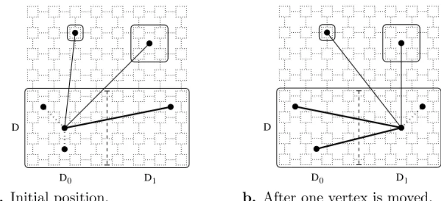
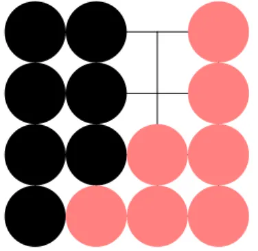
which accounts for the dilation of edges internal to subgraph S′ _{as well as for the} one of edges which belong to the cocycle of S′_{, as shown in Figure 1. Taking into} account the partial mapping results issued by previous bipartitionings makes it pos-sible to avoid local choices that might prove globally bad, as explained below. This amounts to incorporating additional constraints to the standard graph bipartition-ing problem, turnbipartition-ing it into a more general optimization problem termed skewed graph partitioning by some authors [27].

D0 D1

D

a. Initial position.

D0 D1

D

b. After one vertex is moved.

Figure 1: Edges accounted for in the partial communication cost function when bipartitioning the subgraph associated with domain D between the two subdomains D0 and D1 of D. Dotted edges are of dilation zero, their two ends being mapped onto the same subdomain. Thin edges are cocycle edges.

3.1.5 Execution scheme

From an algorithmic point of view, our mapper behaves as a greedy algorithm, since the mapping of a process to a subdomain is never reconsidered, and at each step of which iterative algorithms can be applied. The double recursive call performed at each step induces a recursion scheme in the shape of a binary tree, each vertex of which corresponds to a bipartitioning job, that is, the bipartitioning of both a domain and its associated subgraph.

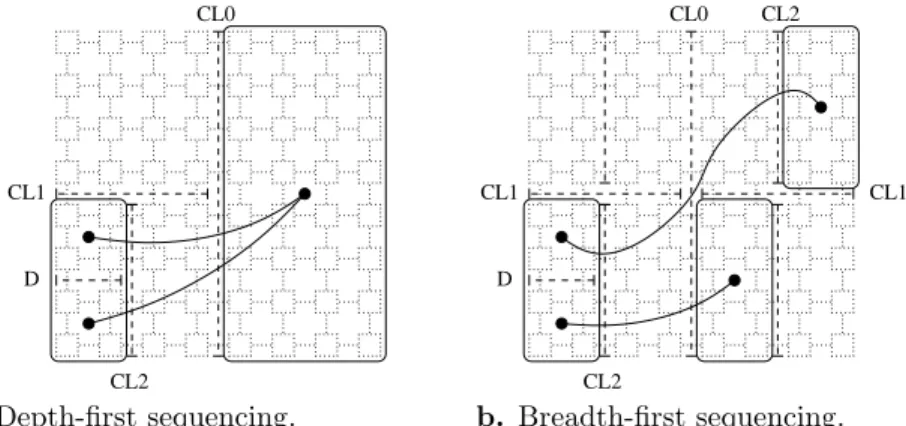
In the case of depth-first sequencing, as written in the above sketch, biparti-tioning jobs run in the left branches of the tree have no information on the dis-tance between the vertices they handle and neighbor vertices to be processed in the right branches. On the contrary, sequencing the jobs according to a by-level (breadth-first) travel of the tree allows any bipartitioning job of a given level to have information on the subdomains to which all the processes have been assigned at the previous level. Thus, when deciding in which subdomain to put a given pro-cess, a bipartitioning job can account for the communication costs induced by its neighbor processes, whether they are handled by the job itself or not, since it can estimate in f′

Cthe dilation of the corresponding edges. This results in an interesting feedback effect: once an edge has been kept in a cut between two subdomains, the distance between its end vertices will be accounted for in the partial communication cost function to be minimized, and following jobs will be more likely to keep these vertices close to each other, as illustrated in Figure 2. The relative efficiency of depth-first and breadth-first sequencing schemes with respect to the structure of the source and target graphs is discussed in [46].

3.1.6 Graph bipartitioning methods

The core of our recursive mapping algorithm uses process graph bipartitioning meth-ods as black boxes. It allows the mapper to run any type of graph bipartitioning method compatible with our criteria for quality. Bipartitioning jobs maintain an in-ternal image of the current bipartition, indicating for every vertex of the job whether it is currently assigned to the first or to the second subdomain. It is therefore possi-ble to apply several different methods in sequence, each one starting from the result of the previous one, and to select the methods with respect to the job character-istics, thus enabling us to define mapping strategies. The currently implemented

D CL2 CL0 CL1 a. Depth-first sequencing. D CL1 CL2 CL0 CL1 CL2 b. Breadth-first sequencing.

Figure 2: Influence of depth-first and breadth-first sequencings on the bipartitioning of a domain D belonging to the leftmost branch of the bipartitioning tree. With breadth-first sequencing, the partial mapping data regarding vertices belonging to the right branches of the bipartitioning tree are more accurate (C.L. stands for “Cut Level”).

graph bipartitioning methods are listed below. Band

Like the multi-level method which will be described below, the band method is a meta-algorithm, in the sense that it does not itself compute partitions, but rather helps other partitioning algorithms perform better. It is a refinement algorithm which, from a given initial partition, extracts a band graph of given width (which only contains graph vertices that are at most at this distance from the separator), calls a partitioning strategy on this band graph, and projects back the refined partition on the original graph. This method was designed to be able to use expensive partitioning heuristics, such as genetic algorithms, on large graphs, as it dramatically reduces the problem space by several orders of magnitude. However, it was found that, in a multi-level context, it also improves partition quality, by coercing partitions in a problem space that derives from the one which was globally defined at the coarsest level, thus preventing local optimization refinement algorithms to be trapped in local optima of the finer graphs [8].

Diffusion

This global optimization method, presented in [44], flows two kinds of antag-onistic liquids, scotch and anti-scotch, from two source vertices, and sets the new frontier as the limit between vertices which contain scotch and the ones which contain anti-scotch. In order to add load-balancing constraints to the algorithm, a constant amount of liquid disappears from every vertex per unit of time, so that no domain can spread across more than half of the vertices. Because selecting the source vertices is essential to the obtainment of use-ful results, this method has been hard-coded so that the two source vertices are the two vertices of highest indices, since in the band method these are the anchor vertices which represent all of the removed vertices of each part. Therefore, this method must be used on band graphs only, or on specifically crafted graphs.

Exactifier

imbal-ance as much as possible, while keeping the value of the communication cost function as small as possible. The vertex set is scanned in order of decreasing vertex weights, and vertices are moved from one subdomain to the other if doing so reduces load imbalance. When several vertices have same weight, the vertex whose swap decreases most the communication cost function is se-lected first. This method is used in post-processing of other methods when load balance is mandatory. For weighted graphs, the strict enforcement of load balance may cause the swapping of isolated vertices of small weight, thus greatly increasing the cut. Therefore, great care should be taken when using this method if connectivity or cut minimization are mandatory.

Fiduccia-Mattheyses

The Fiduccia-Mattheyses heuristics [12] is an almost-linear improvement of the famous Kernighan-Lin algorithm [35]. It tries to improve the bipartition that is input to it by incrementally moving vertices between the subsets of the partition, as long as it can find sequences of moves that lower its commu-nication cost. By considering sequences of moves instead of single swaps, the algorithm allows hill-climbing from local minima of the cost function. As an extension to the original Fiduccia-Mattheyses algorithm, we have developed new data structures, based on logarithmic indexings of arrays, that allow us to handle weighted graphs while preserving the almost-linearity in time of the algorithm [46].

As several authors quoted before [24, 32], the Fiduccia-Mattheyses algorithm gives better results when trying to optimize a good starting partition. There-fore, it should not be used on its own, but rather after greedy starting methods such as the Gibbs-Poole-Stockmeyer or the greedy graph growing methods. Gibbs-Poole-Stockmeyer

This greedy bipartitioning method derives from an algorithm proposed by Gibbs, Poole, and Stockmeyer to minimize the dilation of graph orderings, that is, the maximum absolute value of the difference between the numbers of neighbor vertices [18]. The graph is sliced by using a breadth-first spanning tree rooted at a randomly chosen vertex, and this process is iterated by se-lecting a new root vertex within the last layer as long as the number of layers increases. Then, starting from the current root vertex, vertices are assigned layer after layer to the first subdomain, until half of the total weight has been processed. Remaining vertices are then allocated to the second subdomain. As for the original Gibbs, Poole, and Stockmeyer algorithm, it is assumed that the maximization of the number of layers results in the minimization of the sizes –and therefore of the cocycles– of the layers. This property has already been used by George and Liu to reorder sparse linear systems using the nested dissection method [17], and by Simon in [56].

Greedy graph growing

This greedy algorithm, which has been proposed by Karypis and Kumar [31], belongs to the GRASP (“Greedy Randomized Adaptive Search Procedure”) class [36]. It consists in selecting an initial vertex at random, and repeatedly adding vertices to this growing subset, such that each added vertex results in the smallest increase in the communication cost function. This process, which stops when load balance is achieved, is repeated several times in order to explore (mostly in a gradient-like fashion) different areas of the solution space, and the best partition found is kept.

Multi-level

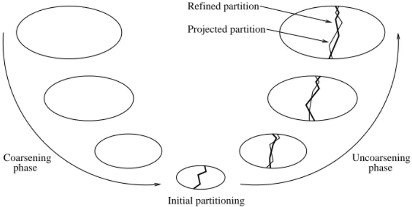
This algorithm, which has been studied by several authors [4, 23, 31] and should be considered as a strategy rather than as a method since it uses other methods as parameters, repeatedly reduces the size of the graph to bipartition by finding matchings that collapse vertices and edges, computes a partition for the coarsest graph obtained, and projects the result back to the original graph, as shown in Figure 3. The multi-level method, when used in

conjunc-Coarsening phase Uncoarsening phase Initial partitioning Projected partition Refined partition

Figure 3: The multi-level partitioning process. In the uncoarsening phase, the light and bold lines represent for each level the projected partition obtained from the coarser graph, and the partition obtained after refinement, respectively.

tion with the Fiduccia-Mattheyses method to compute the initial partitions and refine the projected partitions at every level, usually leads to a signifi-cant improvement in quality with respect to the plain Fiduccia-Mattheyses method. By coarsening the graph used by the Fiduccia-Mattheyses method to compute and project back the initial partition, the multi-level algorithm broadens the scope of the Fiduccia-Mattheyses algorithm, and makes possible for it to account for topological structures of the graph that would else be of a too high level for it to encompass in its local optimization process.

3.1.7 Mapping onto variable-sized architectures

Several constrained graph partitioning problems can be modeled as mapping the problem graph onto a target architecture, the number of vertices and topology of which depend dynamically on the structure of the subgraphs to bipartition at each step.

Variable-sized architectures are supported by the DRB algorithm in the follow-ing way: at the end of each bipartitionfollow-ing step, if any of the variable subdomains is empty (that is, all vertices of the subgraph are mapped only to one of the sub-domains), then the DRB process stops for both subdomains, and all of the vertices are assigned to their parent subdomain; else, if a variable subdomain has only one vertex mapped onto it, the DRB process stops for this subdomain, and the vertex is assigned to it.

The moment when to stop the DRB process for a specific subgraph can be con-trolled by defining a bipartitioning strategy that tests for the validity of a criterion at each bipartitioning step, and maps all of the subgraph vertices to one of the subdomains when it becomes false.

3.2

Sparse matrix ordering by hybrid incomplete nested

dis-section

When solving large sparse linear systems of the form Ax = b, it is common to precede the numerical factorization by a symmetric reordering. This reordering is chosen in such a way that pivoting down the diagonal in order on the resulting permuted matrix P APT _{produces much less fill-in and work than computing the} factors of A by pivoting down the diagonal in the original order (the fill-in is the set of zero entries in A that become non-zero in the factored matrix).

3.2.1 Minimum Degree

The minimum degree algorithm [57] is a local heuristic that performs its pivot selection by iteratively selecting from the graph a node of minimum degree.

The minimum degree algorithm is known to be a very fast and general purpose algorithm, and has received much attention over the last three decades (see for example [1, 16, 41]). However, the algorithm is intrinsically sequential, and very little can be theoretically proved about its efficiency.

3.2.2 Nested dissection

The nested dissection algorithm [17] is a global, heuristic, recursive algorithm which computes a vertex set S that separates the graph into two parts A and B, ordering Swith the highest remaining indices. It then proceeds recursively on parts A and B until their sizes become smaller than some threshold value. This ordering guarantees that, at each step, no non zero term can appear in the factorization process between unknowns of A and unknowns of B.

Many theoretical results have been carried out on nested dissection order-ing [7, 40], and its divide and conquer nature makes it easily parallelizable. The main issue of the nested dissection ordering algorithm is thus to find small vertex separators that balance the remaining subgraphs as evenly as possible. Most often, vertex separators are computed by using direct heuristics [28, 38], or from edge separators [50, and included references] by minimum cover techniques [9, 30], but other techniques such as spectral vertex partitioning have also been used [51].

Provided that good vertex separators are found, the nested dissection algorithm produces orderings which, both in terms of fill-in and operation count, compare favorably [20, 31, 48] to the ones obtained with the minimum degree algorithm [41]. Moreover, the elimination trees induced by nested dissection are broader, shorter, and better balanced, and therefore exhibit much more concurrency in the context of parallel Cholesky factorization [3, 14, 15, 20, 48, 55, and included references]. 3.2.3 Hybridization

Due to their complementary nature, several schemes have been proposed to hybridize the two methods [28, 34, 48]. However, to our knowledge, only loose couplings have been achieved: incomplete nested dissection is performed on the graph to order, and the resulting subgraphs are passed to some minimum degree algorithm. This results in the fact that the minimum degree algorithm does not have exact degree values for all of the boundary vertices of the subgraphs, leading to a misbehavior of the vertex selection process.

Our ordering program implements a tight coupling of the nested dissection and minimum degree algorithms, that allows each of them to take advantage of the infor-mation computed by the other. First, the nested dissection algorithm provides exact degree values for the boundary vertices of the subgraphs passed to the minimum degree algorithm (called halo minimum degree since it has a partial visibility of the neighborhood of the subgraph). Second, the minimum degree algorithm returns the assembly tree that it computes for each subgraph, thus allowing for supervariable amalgamation, in order to obtain column-blocks of a size suitable for BLAS3 block computations.

As for our mapping program, it is possible to combine ordering methods into ordering strategies, which allow the user to select the proper methods with respect to the characteristics of the subgraphs.

The ordering program is completely parametrized by its ordering strategy. The nested dissection method allows the user to take advantage of all of the graph partitioning routines that have been developed in the earlier stages of the Scotch project. Internal ordering strategies for the separators are relevant in the case of sequential or parallel [19, 52, 53, 54] block solving, to select ordering algorithms that minimize the number of extra-diagonal blocks [7], thus allowing for efficient use of BLAS3 primitives, and to reduce inter-processor communication.

3.2.4 Performance criteria

The quality of orderings is evaluated with respect to several criteria. The first one, NNZ, is the number of non-zero terms in the factored reordered matrix. The second one, OPC, is the operation count, that is the number of arithmetic operations required to factor the matrix. The operation count that we have considered takes into consideration all operations (additions, subtractions, multiplications, divisions) required by Cholesky factorization, except square roots; it is equal toP

cn2c, where nc is the number of non-zeros of column c of the factored matrix, diagonal included. A third criterion for quality is the shape of the elimination tree; concurrency in parallel solving is all the higher as the elimination tree is broad and short. To measure its quality, several parameters can be defined: hmin, hmax, and havgdenote the minimum, maximum, and average heights of the tree1_{, respectively, and h}

dlt is the variance, expressed as a percentage of havg. Since small separators result in small chains in the elimination tree, havg should also indirectly reflect the quality of separators.

3.2.5 Ordering methods

The core of our ordering algorithm uses graph ordering methods as black boxes, which allows the orderer to run any type of ordering method. In addition to yielding orderings of the subgraphs that are passed to them, these methods may compute column block partitions of the subgraphs, that are recorded in a separate tree structure. The currently implemented graph ordering methods are listed below. Halo approximate minimum degree

The halo approximate minimum degree method [49] is an improvement of the approximate minimum degree [1] algorithm, suited for use on subgraphs

1_{We do not consider as leaves the disconnected vertices that are present in some meshes, since}

produced by nested dissection methods. Its interest compared to classical min-imum degree algorithms is that boundary vertices are processed using their real degree in the global graph rather than their (much smaller) degree in the subgraph, resulting in smaller fill-in and operation count. This method also implements amalgamation techniques that result in efficient block computa-tions in the factoring and the solving processes.

Halo approximate minimum fill

The halo approximate minimum fill method is a variant of the halo approxi-mate minimum degree algorithm, where the criterion to select the next vertex to permute is not based on its current estimated degree but on the minimiza-tion of the induced fill.

Graph compression

The graph compression method [2] merges cliques of vertices into single nodes, so as to speed-up the ordering of the compressed graph. It also results in some improvement of the quality of separators, especially for stiffness matrices. Gibbs-Poole-Stockmeyer

This method is mainly used on separators to reduce the number and extent of extra-diagonal blocks.

Simple method

Vertices are ordered consecutively, in the same order as they are stored in the graph. This is the fastest method to use on separators when the shape of extra-diagonal structures is not a concern.

Nested dissection

Incomplete nested dissection method. Separators are computed recursively on subgraphs, and specific ordering methods are applied to the separators and to the resulting subgraphs (see sections 3.2.2 and 3.2.3).

3.2.6 Graph separation methods

The core of our incomplete nested dissection algorithm uses graph separation methods as black boxes. It allows the orderer to run any type of graph separation method compatible with our criteria for quality, that is, reducing the size of the vertex separator while maintaining the loads of the separated parts within some user-specified tolerance. Separation jobs maintain an internal image of the current vertex separator, indicating for every vertex of the job whether it is currently assigned to one of the two parts, or to the separator. It is therefore possible to apply several different methods in sequence, each one starting from the result of the previous one, and to select the methods with respect to the job characteristics, thus enabling the definition of separation strategies.

The currently implemented graph separation methods are listed below. Fiduccia-Mattheyses

This is a vertex-oriented version of the original, edge-oriented, Fiduccia-Mattheyses heuristics described in page 13.

Greedy graph growing

This is a vertex-oriented version of the edge-oriented greedy graph growing algorithm described in page 13.

Multi-level

This is a vertex-oriented version of the edge-oriented multi-level algorithm described in page 14.

Thinner

This greedy algorithm refines the current separator by removing all of the exceeding vertices, that is, vertices that do not have neighbors in both parts. It is provided as a simple gradient refinement algorithm for the multi-level method, and is clearly outperformed by the Fiduccia-Mattheyses algorithm. Vertex cover

This algorithm computes a vertex separator by first computing an edge sepa-rator, that is, a bipartition of the graph, and then turning it into a vertex sep-arator by using the method proposed by Pothen and Fang [50]. This method requires the computation of maximal matchings in the bipartite graphs as-sociated with the edge cuts, which are built using Duff’s variant [9] of the Hopcroft and Karp algorithm [30]. Edge separators are computed by using a bipartitioning strategy, which can use any of the graph bipartitioning methods described in section 3.1.6, page 11.

4

Updates

4.1

Changes from version 4.0

Scotch _{has gone parallel with the release of PT-Scotch, the Parallel Threaded} Scotch_{. People interested in these parallel routines should refer to the PT-Scotch} and libScotch 5.1 User’s Guide [45], which extends this manual.

A compatibility library has been developed to allow users to try and use Scotch in programs that were designed to use MeTiS. Please refer to Section 7.14 for more information.

Scotch_{can now handle compressed streams on the fly, in several widely used} formats such as gzip, bzip2 or lzma. Please refer to Section 6.2 for more informa-tion.

5

Files and data structures

For the sake of portability, readability, and reduction of storage space, all the data files shared by the different programs of the Scotch project are coded in plain ASCII text exclusively. Although we may speak of “lines” when describing file for-mats, text-formatting characters such as newlines or tabulations are not mandatory, and are not taken into account when files are read. They are only used to provide better readability and understanding. Whenever numbers are used to label objects, and unless explicitely stated, numberings always start from zero, not one.

5.1

Graph files

Graph files, which usually end in “.grf” or “.src”, describe valuated graphs, which can be valuated process graphs to be mapped onto target architectures, or graphs representing the adjacency structures of matrices to order.

Graphs are represented by means of adjacency lists: the definition of each vertex is accompanied by the list of all of its neighbors, i.e. all of its adjacent arcs.

Therefore, the overall number of edge data is twice the number of edges.

Since version 3.3 has been introduced a new file format, referred to as the “new-style” file format, which replaces the previous, “old-“new-style”, file format. The two advantages of the new-style format over its predecessor are its greater compacity, which results in shorter I/O times, and its ability to handle easily graphs output by C or by Fortran programs.

Starting from version 4.0, only the new format is supported. To convert remaining old-style graph files into new-style graph files, one should get version 3.4 of the Scotch distribution, which comprises the scv file converter, and use it to produce new-style Scotch graph files from the old-style Scotch graph files which it is able to read. See section 6.3.5 for a description of gcv, formerly called scv.

The first line of a graph file holds the graph file version number, which is cur-rently 0. The second line holds the number of vertices of the graph (referred to as vertnbrin libScotch; see for instance Figure 16, page 49, for a detailed example), followed by its number of arcs (unappropriately called edgenbr, as it is in fact equal to twice the actual number of edges). The third line holds two figures: the graph base index value (baseval), and a numeric flag.

The graph base index value records the value of the starting index used to describe the graph; it is usually 0 when the graph has been output by C programs, and 1 for Fortran programs. Its purpose is to ease the manipulation of graphs within each of these two environments, while providing compatibility between them.

The numeric flag, similar to the one used by the Chaco graph format [24], is made of three decimal digits. A non-zero value in the units indicates that vertex weights are provided. A non-zero value in the tenths indicates that edge weights are provided. A non-zero value in the hundredths indicates that vertex labels are provided; if it is the case, vertices can be stored in any order in the file; else, natural order is assumed, starting from the graph base index.

This header data is then followed by as many lines as there are vertices in the graph, that is, vertnbr lines. Each of these lines begins with the vertex label, if necessary, the vertex load, if necessary, and the vertex degree, followed by the description of the arcs. An arc is defined by the load of the edge, if necessary, and by the label of its other end vertex. The arcs of a given vertex can be provided in any order in its neighbor list. If vertex labels are provided, vertices can also be stored in any order in the file.

Figure 4 shows the contents of a graph file modeling a cube with unity vertex and edge weights and base 0.

0 8 24 0 000 3 4 2 1 3 5 3 0 3 6 0 3 3 7 1 2 3 0 6 5 3 1 7 4 3 2 4 7 3 3 5 6

5.2

Mesh files

Mesh files, which usually end in “.msh”, describe valuated meshes, made of elements and nodes, the elements of which can be mapped onto target architectures, and the nodes of which can be reordered.

Meshes are bipartite graphs, in the sense that every element is connected to the nodes that it comprises, and every node is connected to the elements to which it belongs. No edge connects any two element vertices, nor any two node vertices. One can also think of meshes as hypergraphs, such that nodes are the vertices of the hypergraph and elements are hyper-edges which connect multiple nodes, or reciprocally such that elements are the vertices of the hypergraph and nodes are hyper-edges which connect multiple elements.

Since meshes are graphs, the structure of mesh files resembles very much the one of graph files described above in section 5.1, and differs only by its header, which indicates which of the vertices are node vertices and element vertices.

The first line of a mesh file holds the mesh file version number, which is currently 1. Graph and mesh version numbers will always differ, which enables application programs to accept both file formats and adapt their behavior according to the type of input data. The second line holds the number of elements of the mesh (velmnbr), followed by its number of nodes (vnodnbr), and by its overall number of arcs (edgenbr, that is, twice the number of edges which connect elements to nodes and vice-versa).

The third line holds three figures: the base index of the first element vertex in memory (velmbas), the base index of the first node vertex in memory (vnodbas), and a numeric flag.

The Scotch mesh file format requires that all nodes and all elements be assigned to contiguous ranges of indices. Therefore, either all element vertices are defined before all node vertices, or all node vertices are defined before all element vertices. The node and element base indices indicate at the same time whether elements or nodes are put in the first place, as well as the value of the starting index used to describe the graph. Indeed, if velmbas < vnodbas, then elements have the smallest indices, velmbas is the base value of the underlying graph (that is, baseval = velmbas), and velmbas + velmnbr = vnodbas holds. Conversely, if velmbas > vnodbas, then nodes have the smallest indices, vnodbas is the base value of the underlying graph, (that is, baseval = vnodbas), and vnodbas+vnodnbr = velmbas holds.

The numeric flag, similar to the one used by the Chaco graph format [24], is made of three decimal digits. A non-zero value in the units indicates that vertex weights are provided. A non-zero value in the tenths indicates that edge weights are provided. A non-zero value in the hundredths indicates that vertex labels are provided; if it is the case, and if velmbas < vnodbas (resp. velmbas > vnodbas), the velmnbr (resp. vnodnbr) first vertex lines are assumed to be element (resp. node) vertices, irrespective of their vertex labels, and the vnodnbr (resp. velmnbr) remaining vertex lines are assumed to be node (resp. element) vertices; else, natural order is assumed, starting at the underlying graph base index (baseval).

This header data is then followed by as many lines as there are node and element vertices in the graph. These lines are similar to the ones of the graph format, except that, in order to save disk space, the numberings of nodes and elements all start from the same base value, that is, min(velmbas, vnodbas) (also called baseval, like for regular graphs).

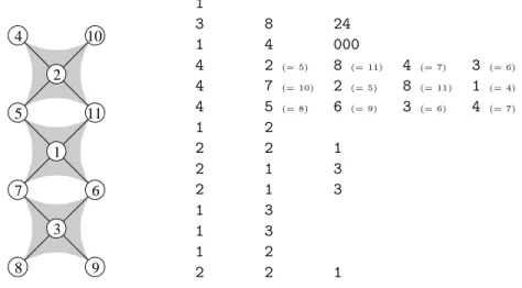
For example, Figure 5 shows the contents of the mesh file modeling three square elements, with unity vertex and edge weights, elements defined before nodes, and numbering of the underlying graph starting from 1. In memory, the three elements are labeled from 1 to 3, and the eight nodes are labeled from 4 to 11. In the file, the three elements are still labeled from 1 to 3, while the eight nodes are labeled from 1 to 8.

When labels are used, elements and nodes may have similar labels, but not two elements, nor two nodes, should have the same labels.

4 2 5 1 6 3 10 11 7 8 9 1 3 8 24 1 4 000 4 2 (= 5) 8 (= 11) 4 (= 7) 3 (= 6) 4 7 (= 10) 2 (= 5) 8 (= 11) 1 (= 4) 4 5 (= 8) 6 (= 9) 3 (= 6) 4 (= 7) 1 2 2 2 1 2 1 3 2 1 3 1 3 1 3 1 2 2 2 1

Figure 5: Mesh file representing three square elements, with unity vertex and edge weights. Elements are defined before nodes, and numbering of the underlying graph starts from 1. The left part of the figure shows the mesh representation in memory, with consecutive element and node indices. The right part of the figure shows the contents of the file, with both element and node numberings starting from 1, the minimum of the element and node base values. Corresponding node indices in memory are shown in parentheses for the sake of comprehension.

5.3

Geometry files

Geometry files, which usually end in “.xyz”, hold the coordinates of the vertices of their associated graph or mesh. These files are not used in the mapping process itself, since only topological properties are taken into account then (mappings are computed regardless of graph geometry). They are used by visualization programs to compute graphical representations of mapping results.

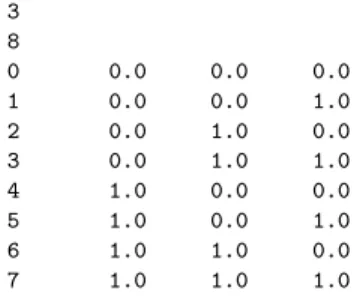
The first string to appear in a geometry file codes for its type, or dimensional-ity. It is “1” if the file contains unidimensional coordinates, “2” for bidimensional coordinates, and “3” for tridimensional coordinates. It is followed by the number of coordinate data stored in the file, which should be at least equal to the number of vertices of the associated graph or mesh, and by that many coordinate lines. Each coordinate line holds the label of the vertex, plus one, two or three real numbers which are the (X), (X,Y), or (X,Y,Z), coordinates of the graph vertices, according to the graph dimensionality.

Vertices can be stored in any order in the file. Moreover, a geometry file can have more coordinate data than there are vertices in the associated graph or mesh file; only coordinates the labels of which match labels of graph or mesh vertices will be

taken into account. This feature allows all subgraphs of a given graph or mesh to share the same geometry file, provided that graph vertex labels remain unchanged. For example, Figure 6 shows the contents of the 3D geometry file associated with the graph of Figure 4.

3 8 0 0.0 0.0 0.0 1 0.0 0.0 1.0 2 0.0 1.0 0.0 3 0.0 1.0 1.0 4 1.0 0.0 0.0 5 1.0 0.0 1.0 6 1.0 1.0 0.0 7 1.0 1.0 1.0

Figure 6: Geometry file associated with the graph file of Figure 4.

5.4

Target files

Target files describe the architectures onto which source graphs are mapped. Instead of containing the structure of the target graph itself, as source graph files do, target files define how target graphs are bipartitioned and give the distances between all pairs of vertices (that is, processors). Keeping the bipartitioning information within target files avoids recomputing it every time a target architecture is used. We are allowed to do so because, in our approach, the recursive bipartitioning of the target graph is fully independent with respect to that of the source graph (however, the opposite is false).

For space and time saving issues, some classical homogeneous architectures (2D and 3D meshes and tori, hypercubes, complete graphs, etc.) have been algorithmi-cally coded within the mapper itself by the means of built-in functions. Instead of containing the whole graph decomposition data, their target files hold only a few values, used as parameters by the built-in functions.

5.4.1 Decomposition-defined architecture files

Decomposition-defined architecture files are the standard way to describe weighted and/or irregular target architectures. Several file formats exist, but we only present here the most humanly readable one, which begins in “deco 0” (“deco” stands for “decomposition-defined” architecture, and “0” is the format type).

The “deco 0” header is followed by two integer numbers, which are the number of processors and the largest terminal number used in the decomposition, respec-tively. Two arrays follow. The first array has as many lines as there are processors. Each of these lines holds three numbers: the processor label, the processor weight (that is an estimation of its computational power), and its terminal number. The terminal number associated with every processor is obtained by giving the initial domain holding all the processors number 1, and by numbering the two subdomains of a given domain of number i with numbers 2i and 2i + 1. The second array is a lower triangular diagonal-less matrix that gives the distance between all pairs of processors. This distance matrix, combined with the decomposition tree coded by terminal numbers, allows the evaluation by averaging of the distance between all pairs of domains. In order for the mapper to behave properly, distances between

processors must be strictly positive numbers. Therefore, null distances are not ac-cepted. For instance, Figure 7 shows the contents of the architecture decomposition file for UB(2, 3), the binary de Bruijn graph of dimension 3, as computed by the amk grfprogram.

1

7

3

6

12 13

9 11

8 10

5

4

2

14

15

Figure 7: Target decomposition file for UB(2, 3). The terminal numbers associated with every processor define a unique recursive bipartitioning of the target graph.

5.4.2 Algorithmically-coded architecture files

All algorithmically-coded architectures are defined with unity edge and vertex weights. They start with an abbreviation name of the architecture, followed by parameters specific to the architecture. The available built-in architecture defini-tions are listed below.

cmplt size

Defines a complete graph with size vertices. The vertex labels are numbers between 0 and size − 1.

cmpltw size load0 load1. . . loadsize₋₁

Defines a weighted complete graph with size vertices. The vertex labels are numbers between 0 and size − 1, and vertices are assigned integer weights in the order in which these are provided.

hcub dim

Defines a binary hypercube of dimension dim. The vertex labels are the decimal values of the binary representations of the vertex coordinates in the hypercube.

leaf height cluster weight

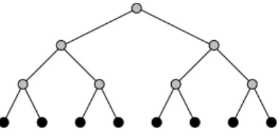
Defines a tree-leaf architecture with height levels and 2height vertices. The tree-leaf graph models a machine the topology of which is a complete binary tree, such that leaves are processors and all other nodes are communication routers, as shown in Figure 8. Only the leaves are used to map processes, but distances between them are computed by considering the whole tree. This graph is used to represent multi-stage machines with constant bandwidth,

Figure 8: The “tree-leaf” graph of height 3. Processors are drawn in black and routers in grey.

such as the CM-5 [37] for which experiments have shown that bandwidth is constant between every pair of processors and hardly depends on network congestion [39], or the SP-2 with power-of-two number of nodes.

The two additional parameters cluster and weight serve to model hetero-geneous architectures for which multiprocessor nodes having several highly interconnected processors (typically by means of shared memory) are linked by means of networks of lower bandwidth. cluster represents the number of levels to traverse, starting from the root of the leaf, before reaching the multiprocessors, each multiprocessor having 2height−cluster nodes. weight is the relative cost of extra-cluster links, that is, links in the upper levels of the tree-leaf graph. Links within clusters are assumed to have weight 1.

When there are no clusters at all, that is, in the case of purely homogeneous architectures, set cluster to be equal to height, and weight to 1.

mesh2D dimX dimY

Defines a bidimensional array of dimX columns by dimY rows. The vertex with coordinates (posX, posY) has label posY × dimX + posX.

mesh3D dimX dimY dimZ

Defines a tridimensional array of dimX columns by dimY rows by dimZ lev-els. The vertex with coordinates (posX,posY,posZ ) has label (posZ × dimY + posY) × dimX + posX.

torus2D dimX dimY

Defines a bidimensional array of dimX columns by dimY rows, with wraparound edges. The vertex with coordinates (posX, posY) has label posY× dimX + posX.

torus3D dimX dimY dimZ

Defines a tridimensional array of dimX columns by dimY rows by dimZ levels, with wraparound edges. The vertex with coordinates (posX,posY,posZ ) has label (posZ × dimY + posY) × dimX + posX.

5.4.3 Variable-sized architecture files

Variable-sized architectures are a class of algorithmically-coded architectures the size of which is not defined a priori. As for fixed-size algorithmically-coded ar-chitectures, they start with an abbreviation name of the architecture, followed by parameters specific to the architecture. The available built-in variable-sized archi-tecture definitions are listed below.

varcmplt

Defines a variable-sized complete graph. Domains are labeled such that the first domain is labeled 1, and the two subdomains of any domain i are labeled

2i and 2i + 1. The distance between any two subdomains i and j is 0 if i = j and 1 else.

varhcub

Defines a variable-sized hypercube. Domains are labeled such that the first domain is labeled 1, and the two subdomains of any domain i are labeled 2i and 2i + 1. The distance between any two domains is the Hamming distance between the common bits of the two domains, plus half of the absolute dif-ference between the levels of the two domains, this latter term modeling the average distance on unknown bits. For instance, the distance between subdo-main 9 = 1001B, of level 3 (since its leftmost 1 has been shifted left thrice), and subdomain 53 = 110101B, of level 5 (since its leftmost 1 has been shifted left five times), is 2: it is 1, which is the number of bits which differ between 1101B (that is, 53 = 110101B shifted rightwards twice) and 1001B, plus 1, which is half of the absolute difference between 5 and 3.

5.5

Mapping files

Mapping files, which usually end in “.map”, contain the result of the mapping of source graphs onto target architectures. They associate a vertex of the target graph with every vertex of the source graph.

Mapping files begin with the number of mapping lines which they contain, fol-lowed by that many mapping lines. Each mapping line holds a mapping pair, made of two integer numbers which are the label of a source graph vertex and the label of the target graph vertex onto which it is mapped. Mapping pairs can be stored in any order in the file; however, labels of source graph vertices must be all dif-ferent. For example, Figure 9 shows the result obtained when mapping the source graph of Figure 4 onto the target architecture of Figure 7. This one-to-one embed-ding of H(3) into UB(2, 3) has dilation 1, except for one hypercube edge which has dilation 3. 8 0 1 1 3 2 2 3 5 4 0 5 7 6 4 7 6

Figure 9: Mapping file obtained when mapping the hypercube source graph of Figure 4 onto the binary de Bruijn architecture of Figure 7.

Mapping files are also used on output of the block orderer to represent the allocation of the vertices of the original graph to the column blocks associated with the ordering. In this case, column blocks are labeled in ascending order, such that the number of a block is always greater than the ones of its predecessors in the elimination process, that is, its leaves in the elimination tree.

5.6

Ordering files

Ordering files, which usually end in “.ord”, contain the result of the ordering of source graphs or meshes that represent sparse matrices. They associate a number

with every vertex of the source graph or mesh.

The structure of ordering files is analogous to the one of mapping files; they differ only by the meaning of their data.

Ordering files begin with the number of ordering lines which they contain, that is the number of vertices in the source graph or the number of nodes in the source mesh, followed by that many ordering lines. Each ordering line holds an ordering pair, made of two integer numbers which are the label of a source graph or mesh vertex and its rank in the ordering. Ranks range from the base value of the graph or mesh (baseval) to the base value plus the number of vertices (resp. nodes), minus one (baseval + vertnbr − 1 for graphs, and baseval + vnodnbr − 1 for meshes). Ordering pairs can be stored in any order in the file; however, indices of source vertices must be all different.

For example, Figure 10 shows the result obtained when reordering the source graph of Figure 4. 8 0 6 1 3 2 2 3 7 4 1 5 5 6 4 7 0

Figure 10: Ordering file obtained when reordering the hypercube graph of Figure 4. The advantage of having both graph and mesh orderings start from baseval (and not vnodbas in the case of meshes) is that an ordering computed on the nodal graph of some mesh has the same structure as an ordering computed from the native mesh structure, allowing for greater modularity. However, in memory, permutation indices for meshes are numbered from vnodbas to vnodbas + vnodnbr − 1.

5.7

Vertex list files

Vertex lists are used by programs that select vertices from graphs.

Vertex lists are coded as lists of integer numbers. The first integer is the number of vertices in the list and the other integers are the labels of the selected vertices, given in any order. For example, Figure 11 shows the list made from three vertices of labels 2, 45, and 7.

3 2 45 7

Figure 11: Example of vertex list with three vertices of labels 2, 45, and 7.

6

Programs

The programs of the Scotch project belong to five distinct classes.

• Graph handling programs, the names of which begin in “g”, that serve to build and test source graphs.

• Mesh handling programs, the names of which begin in “m”, that serve to build and test source meshes.

• Target architecture handling programs, the names of which begin in “a”, that allow the user to build and test decomposition-defined target files, and especially to turn a source graph file into a target file.

• The mapping and ordering programs themselves.

• Output handling programs, which are the mapping performance analyzer, the graph factorization program, and the graph, matrix, and mapping visualiza-tion program.

The general architecture of the Scotch project is displayed in Figure 12.

6.1

Invocation

The programs comprising the Scotch project have been designed to run in command-line mode without any interactive prompting, so that they can be called easily from other programs by means of “system ()” or “popen ()” system calls, or be piped together on a single shell command line. In order to facilitate this, whenever a stream name is asked for (either on input or output), the user may put a single “-” to indicate standard input or output. Moreover, programs read their input in the same order as stream names are given in the command line. It allows them to read all their data from a single stream (usually the standard input), provided that these data are ordered properly.

A brief on-line help is provided with all the programs. To get this help, use the “-h” option after the program name. The case of option letters is not significant, except when both the lower and upper cases of a letter have different meanings. When passing parameters to the programs, only the order of file names is significant; options can be put anywhere in the command line, in any order. Examples of use of the different programs of the Scotch project are provided in section 9.

Error messages are standardized, but may not be fully explanatory. However, most of the errors you may run into should be related to file formats, and located in “...Load” routines. In this case, compare your data formats with the definitions given in section 5, and use the gtst and mtst programs to check the consistency of source graphs and meshes.

6.2

Using compressed files

Starting from version 5.0.6, Scotch allows users to provide and retrieve data in compressed form. Since this feature requires that the compression and decompres-sion tasks run in the same time as data is read or written, it can only be done on systems which support multi-threading (Posix threads) or multi-processing (by means of fork system calls).

To determine if a stream has to be handled in compressed form, Scotch checks its extension. If it is “.gz” (gzip format), “.bz2” (bzip2 format) or “.lzma” (lzma format), the stream is assumed to be compressed according to the corresponding format. A filter task will then be used to process it accordingly if the format is implemented in Scotch and enabled on your system.

To date, data can be read and written in bzip2 and gzip formats, and can also be read in the lzma format. Since the compression ratio of lzma on Scotch graphs is 30% better than the one of gzip and bzip2 (which are almost equivalent

Program File Source graph file .grf mtst .tgt Target file gtst atst .msh Source mesh file mord External graph file gcv External mesh file mmk_* gmk_* mcv .xyz Geometry file gord gmk_msh file .ord Ordering file Mapping .map gmtst file Graphics gout amk_grf gotst acpl amk_* gmap Data flow

Figure 12: General architecture of the Scotch project. All of the features offered by the stand-alone programs are also available in the libScotch library.

in this case), the lzma format is a very good choice for handling very large graphs. To see how to enable compressed data handling in Scotch, please refer to Section 8. When the compressed format allows it, several files can be provided on the same stream, and be uncompressed on the fly. For instance, the command “cat brol.grf.gz brol.xyz.gz | gout -.gz -.gz -Mn - brol.iv” concatenates the topology and geometry data of some graph brol and feed them as a single compressed stream to the standard input of program gout, hence the ”-.gz” to indicate a compressed standard stream.

6.3

Description

Synopsis

acpl[input target file [output target file]] options Description

The program acpl is the decomposition-defined architecture file compiler. It processes architecture files of type “deco 0” built by hand or by the amk * programs, to create a “deco 1” compiled architecture file of about four times the size of the original one; see section 5.4.1, page 22, for a detailed description of decomposition-defined target architecture file formats.

The mapper can read both original and compiled architecture file formats. However, compiled architecture files are read much more efficiently, as they are directly loaded into memory without further processing. Since the compilation time of a target architecture graph evolves as the square of its number of vertices, precompiling with acpl can save some time when many mappings are to be performed onto the same large target architecture.

Options

-h Display the program synopsis.

-V Print the program version and copyright. 6.3.2 amk *

Synopsis

amk ccc dim[output target file] options amk fft2 dim[output target file] options amk hy dim[output target file] options

amk m2 dimX[dimY [output target file]] options amk p2 weight0[weight1 [output target file]] options

Description