Publisher’s version / Version de l'éditeur:
Vous avez des questions? Nous pouvons vous aider. Pour communiquer directement avec un auteur, consultez la première page de la revue dans laquelle son article a été publié afin de trouver ses coordonnées. Si vous n’arrivez pas à les repérer, communiquez avec nous à PublicationsArchive-ArchivesPublications@nrc-cnrc.gc.ca.
Questions? Contact the NRC Publications Archive team at
PublicationsArchive-ArchivesPublications@nrc-cnrc.gc.ca. If you wish to email the authors directly, please see the first page of the publication for their contact information.
https://publications-cnrc.canada.ca/fra/droits
L’accès à ce site Web et l’utilisation de son contenu sont assujettis aux conditions présentées dans le site
LISEZ CES CONDITIONS ATTENTIVEMENT AVANT D’UTILISER CE SITE WEB.
MONET Workshop on Model-Based Systems at 16th European Conference on
Artificial Intelligence [Proceedings], 2004
READ THESE TERMS AND CONDITIONS CAREFULLY BEFORE USING THIS WEBSITE. https://nrc-publications.canada.ca/eng/copyright
NRC Publications Archive Record / Notice des Archives des publications du CNRC :
https://nrc-publications.canada.ca/eng/view/object/?id=fdc9d8e3-1b15-42aa-8d58-30434d53c3bf
https://publications-cnrc.canada.ca/fra/voir/objet/?id=fdc9d8e3-1b15-42aa-8d58-30434d53c3bf
NRC Publications Archive
Archives des publications du CNRC
This publication could be one of several versions: author’s original, accepted manuscript or the publisher’s version. / La version de cette publication peut être l’une des suivantes : la version prépublication de l’auteur, la version acceptée du manuscrit ou la version de l’éditeur.
Access and use of this website and the material on it are subject to the Terms and Conditions set forth at
Sensor Placement and Diagnosability Analysis at Design Stage
Yan, Y.
National Research Council Canada Institute for Information Technology Conseil national de recherches Canada Institut de technologie de l'information
Sensor Placement and Diagnosability Analysis
at Design Stage *
Yan, Y.
August 2004
* published in the MONET Workshop on Model-Based Systems at 16th European
Conference on Artificial Intelligence. August 22-26, 2004. Valencia, Spain. NRC 47160.
Copyright 2004 by
National Research Council of Canada
Permission is granted to quote short excerpts and to reproduce figures and tables from this report, provided that the source of such material is fully acknowledged.
Sensor Placement and Diagnosability
Analysis at Design Stage
Yuhong Yan
1Abstract. Adequate sensors are a necessary condition for fault
di-agnosability. Sensor placement for diagnosis task is to study where to put the sensors so that they are the minimal set to diagnose cer-tain faults. This paper presents a method of sensor placement based on diagnosability analysis using the simulation model in the CAD environment. The fault signature matrix is determined by the projec-tions of different operation modes on observable variables. The min-imal sensor set for detecting faults and for discriminating the faults can be computed from the fault signature matrix. We also consider that values of exogenous variables are a condition for diagnosabil-ity. By introducing the concept of virtual sensors, faults can be de-tectable/discriminable based on their signatures on virtual sensors. The advantages of this approach are that not only the minimal sen-sor set but also the conditions of causal scopes are obtained and the procedure is fully automated.
1
INTRODUCTION
There are demands on the automobile industry to consider vehicle maintenance and diagnosis at the early stage of design. The IDD (In-tegrated Diagnosis and Design) project, a V framework EU project, aims at the definition of a new design process for automotive sys-tems. The goal is to integrate the process of diagnostic development (FMEA, diagnosability analysis, etc.) in the early phase of the de-sign process. Sensor placement for diagnosis task is to study where to put the sensors so that they are the minimal set to diagnose cer-tain faults. The diagnosis principles reveal that diagnosability of the faults relies on adequate sensors to provide redundancy relations so that the discrepancies of the predictions and the observations can be detected. This paper presents a method of sensor placement based on diagnosability analysis using the simulation model in the CAD environment.
A. Short View of Sensor Placement Methods
The criteria for making sensor location decisions vary depending on the goals of the task. In control theory, the sensor network is to provide necessary information for the control of the process or the system, so the study starts from the observability/controllability of the variables. Madorn and Veverka [6] addressed sensor placement for a linear process. Their method makes use of the Gauss-Jordan elimination to identify a minimum set of variables that need to be measured in order to observe all important variables while simultane-ously minimizing the overall cost of sensors. Others consider sensor failures and their effect on the observability of variables. [1] intro-duced the concept of reliability of the estimation of a variable, which
1NRC-IIT-Fredericton, Canada, email: yuhong.yan@nrc.gc.ca
In ECAI 2004 MONET Workshop on Model-Based Systems, Valencia, Spain.
gives the probability of estimating a variable for any given sensor network and specified sensor failure probabilities. [2] discussed the redundancy of sensor network, i.e. more sensors than the minimum to ensure the observabilities of variables when some sensors fail. Simi-lar work can be found in [5].
This paper is in the model-based diagnosis domain. The goal of sensor placement is to achieve the diagnosability, i.e. the sensor net-work can detect and discriminate the faults of the components in a system. Sensor failure is not considered in this paper. The observ-ables from the point of view of diagnosis are the variobserv-ables that can be measured by sensors. This differs from the concept of control the-ory, where the observable variables are the measurable variables plus the unmeasured variables deducible from the measurable variables. Though the terms used in the two domains are similar, the work in this paper has little relation to the work described in the previous paragraph.
Existing work of sensor placement in diagnosis is based on the An-alytical Redundancy Relation (ARR) in [3]. In [9], AND-OR Graph is drawn to show the dependency relation of a potential sensor and components (faults). Then the HFS (Hypothetical Fault Signature) matrix is built to analyse the redundant relation. HFS makes a corre-spondence among the additional sensor, the resulting redundant rela-tion and the involved component. The next step is to build an EHFS (Extended Hypothetical Fault Signature) matrix. This latter matrix takes into account the addition of several sensors at one time. If one independent redundant relation is added by one additional sensor and involves one component, the fault on this component is discrim-inable. Though [9] presents appropriate conclusions, it is not easy to use in practice because its complexity is beyond what an expert can handle for even a small system.
B. Our Approach
Our analysis is based on diagnosability analysis [8]. Intuitively, if the faulty behavior and the normal behavior have disjointed projec-tions on some observables, the fault can be detected; similarly,if two faults have disjointed projections on some observables, the two faults can be discriminated.
Inspired by the signature of ARR, the projections of different modes on the observables can be encoded into {0,1}, based on wether the fault modes have the same or different values to the right mode. This gives a signature for each mode. Therefore, if different modes have different signatures, those modes can be discriminated.
The values of exogenous variables and and/or inputs play a role in diagnosability, i.e. a fault can only be detected under certain do-mains. [8] implies that the domains of the variables can be partitioned into serval areas that have different diagnosability. “Causal scope” is used to represent the partitioned domains. A physical sensor work-ing under different causal scopes can be mapped to several virtual
sensors. Then the fault signatures are built on the virtual sensors. The minimal sensor set for detecting faults and for discriminating the faults can be computed from the fault signature matrix. It is an initial work that the domains of variables are taken into consideration for sensor placement.
When the sensor placement analysis is conducted in the CAD en-vironment, the nature of the simulation function of the CAD envi-ronment actually does the work of constraint propagation. Thus we avoid the complex manual method to build the dependency relation between variables and components as in [9]. Therefore, the method developed in this paper can be conducted fully automatically inside CAD environment.
Section 2 discusses the diagnosability analysis; section 3 presents the approach of sensor placement; section 4 is a small demonstration; and section 5 contains the conclusions.
2
DIAGNOSABILITY ANALYSIS
From the diagnosis principle, a fault modifies the normal behavior of a component, thus generates a discrepancy on the outputs of the com-ponent. The discrepancy propagates by the components links until the discrepancy is detected by sensors on the observable points. Di-agnosability includes two notions[8]: Fault Detectability is whether and under which circumstances the possible faults considered can be distinguished from the right modes; Fault Discriminability is whether and under which circumstances the faults (or the classes of faults) can be distinguished. Discriminability is a stronger defini-tion. The diagnosability is computed from the projections of different modes on the observables [8]:
SITo−cause= P ROJo−cause(OP Ci)\P ROJo−cause(
P ROJobs(M ODELmode1∩OP Ci)∩P ROJobs(M ODELmode2
∩ OP Ci)) (1)
where P ROJ is projection operation, OP C represents operating conditions, and Vobs is observables set. Vobs are divided into two
sets: Vo−causewhich is the set of exogenous or “causal” variables
in Vobs, and Vobs\cause which is the set of rest variables in Vobs.
Mode1 and mode2 are the two modes. SITo−causeis the range of
Vo−cause that the two modes are discriminable. It is calculated in
this way: calculate the projections on the Vobsfor the two modes
(by “P ROJobs”); calculate the conjunction of the two projections
(by “∩” between the two “P ROJobs”); calculate the subtraction of
the projection on Vo−cause of the original modes and the
projec-tion of the conjuncprojec-tion on Vo−cause(by “\”). OP Ciis the variable
to describe different states of the system and its control. Examples are engine idle, clutch engaged, cold engine. For diagnosability, it is meaningful to compare the two modes only when the operating con-ditions are the same. In modeling, it is difficult to distinguish OP C and Vo−causeas long as OP C variables are observable. It is solely
a matter of convenience.
The principle in (1) is that, if the projections on Vobsare disjoint,
the discrepancy of the two modes can be observed, which is called deterministically discriminable (DD). [8] also defines two other cat-egories of discriminability: possibly discriminable (PD), and non-discriminable (ND). We are only concerned with DD in this paper.
The goal of our project, as introduced in Section 1, is to integrate diagnostic tasks at system design time. The system model is available in the CAD environment. Matlab/Simulink is the target platform in our project because of its popularity in automobile industry. Design engineers normally have excellent knowledge of fault modes and an-alyze the fault effects by simulation. The approach developed in this paper assumes that the knowledge of fault modes is available.
Figure 1. values propagate through component links.
Figure 1(a) is a system that contains two components, Comp1 and Comp2. v1,v2, and v3 are their input and output variables, among
them v1and v3 are observables (surrounded by the dotted square).
Comp1 and Comp2 have function as q1: v17→ v2and q2: v27→ v3.
Qualitatively, when Comp1 and Comp2 are both in right modes, they map qualitative tuples as shown in Figure 1(b): q1maps [va, vb] to
[vc, vd], and q2 maps [vc, vd] to [ve, vf]. When Comp1 has fault,
its model changes to q01. q 0 1 maps [va, vb] to [vc0, v 0 d] , and q2 maps [vc0, v 0 d] to [v 0 e, v 0
f] , which is shown in figure 1(c). The graph, as
shown in Figure 1(b) or (c), is called a Tuple Mapping Graph and displays the qualitative relations. In practice, we don’t normally draw such a picture. Through the method in [10], the qualitative model is abstracted from the numerical model automatically in the simulation environment. Therefore, we can use the qualitative relations in the following context directly.
If we want to compare our method with other method where the structural knowledge is used to set up the relation between faults and components, we can find that simulation indeed does the work of constraint propagation, in which the values of variable are propa-gated through the links of components. Therefore, we can obtain the relation of sensor and components (faults) without structural knowl-edge. One can argue that the simulation model does have the struc-tural knowledge about the connections of the components. But we don’t make extra effort to find how the discrepancy is propagated through the connections. The simulation does it for us. The method developed here takes the advantage of the CAD environment and can be integrated into the CAD environment to provide an automatic analysis of sensor placement.
We observe that the modes actually have the same values for vari-ables in Vo−cause, thus the diagnosability analysis reduced into
com-parison of projection on Vobs\cause. In Figure 1, assume is the only element in Vo−cause and is the only element in Vobs\cause, since
takes the same value of , the necessary and sufficient condition of DD is that [ve, vf] ∩ [ve0, v
0
f] = ∅. It is obvious that the values of
Vo−cause is a condition of diagnosability. We call the intervals of
Vo−cause”causal scope”.
Definition 1 (Projection from causal scope) a qualitative relation
q : v 7→ u projection on variable u under causal scope va= [vx, vy]
is U = {∪ui| q : va7→ ui}
Definition 1 says that q : v 7→ u maps vato several ui, the union
of ui is the projection of q under the scope of va = [vx, vy]. The
importance of definition 1 is in including the causal scope vaas a
condition of projection.
Proposition 1 (Discriminability within causal scope) two modes
pro-jections of q1 and q2 on u under a causal scope va = [vx, vy] are
disjoint as U 1 ∩ U 2 = ∅, modes q1 and q2 are discriminable by u under scope va.
The proof is quite straightforward and eliminated here. Proposi-tion 1 says that if the qualitative models for two behavior modes take the same value for Vo−cause, the necessary and sufficient condition
for DD is that the projections on Vobs\causeare disjointed.
3
SENSOR PLACEMENT ANALYSIS
3.1
Minimal Sensor Set
Our approach is inspired by ARR which uses a fault signature matrix to discriminate faults [4]. The difference is that our fault detectability matrix is built on projections. More specifically, since the variables in Vo−causealways take the same values for different modes, the fault
signature matrix is built on Vobs\cause. In order to present the values of Vo−causeas the condition of diagnosability, we define:
Definition 2 (V-sensor) a virtual sensor is a physical sensor
associ-ated with a causal scope.
V-sensor is written as VS(v, scope), where v is the physical vari-able that the sensor measures; the scope is a qualitative value of Vo−cause(can be multi-dimension).
Using definition 2, a physical sensor may be mapped to several V-sensors if the causal scopes are different. For example, assume a sensor S1measures variable v1. Then its V-sensors can be VS1(v1,
scope1) and VS2(v1, scope2), where scope1 and scope2 are two
dif-ferent causal scopes. A fault can be detectable under a certain causal scope but not the others. Using V-sensor gives us a more precise view on sensor placement.
Definition 3 (Fault Detectability Signature): Given a vector of
V-sensors VS={VS1, VS2,...,VSn}, the detectability signature of fault
fjis a binary vector FSj= [s1j,s2j,...snj] in which siis given by :
VS× FS 7→{0,1}
where(VSi, FSj)7→ sij=1 if fjcauses discrepancy at VSi; sij=0 if fj
causes no discrepancy at VSi;
Computing Fault Detectability Signature: discrepancy is
com-puted by the intersection of the values of VSiat mode fjand at right
mode r, i.e.:
if value(VSi| fj)∩ value(VSi| r) =∅, sij= 1
if value(VSi| fj)∩ value(VSi| r) 6= ∅, sij= 0
It is obvious that for the right mode, all the elements in the vector are 0. Table 1 is an example of fault detectability signature matrix.
Table 1. fault detectability signature matrix F1 F2 F3 F4 F5 VS1(v1,scope1) 0 0 0 0 0 VS2(v2,scope2) 1 1 1 0 1 VS3(v3,scope3) 1 1 1 0 1 VS4(v4,scope4) 1 0 1 1 1 VS5(v5,scope5) 0 1 1 1 0
Computing minimal sensor set to detect fault fj: It is easy to
know that one sij=1 is sufficient to detect the fault. The minimal
sensor set (MSS) to detect fault fjis
MSSij= {VSi} with sij=1
All MSSijdefines a set MSSSj={MSSij}.
Example 1: (Get MSSS (MSS Sets) for detecting a fault)
From table 1, the MSSS for detecting F1 is MSSS1={{VS2}, {VS3}, {VS4}}
the MSSSs for F2, F3, F4 and F5 respectively are MSSS2={{VS2}, {VS3}, {VS5}}
MSSS3={{VS2}, {VS3}, {VS4}, {VS5}}
MSSS4={{VS4}, {VS5}}
MSSS5={{VS2}, {VS3}, {VS4}}
Detectability is about discriminating a fault from normal be-haviour. A detectable fault may or may not be discriminated from other faults. To discriminate multiple faults, we have proposition 2:
Proposition 2 If the two faults have different fault detectability
sig-natures, they are discriminable.
Proof: If the two modes have different signatures, there exists at least
one V-sensor taking value 0 in one mode and value 1 in the other. The projections on Vobsof the two modes, for the causal scope defined
by the V-sensor, are thus disjoint (by definition 3). These modes are thus discriminable.
Example 2: (faults with different signatures are discriminable)
Using table 1, for F1 the signature is FS1 = {0, 1, 1, 1, 0} and F2’s signature is FS2 = {0, 1, 1, 0, 1}. Since FS1 6= FS2, the two faults are discriminable. For F1 and F5, since their signatures are equal, the two faults are not discriminable.
Remark of Proposition 2: Proposition 2 gives sufficient conditions of discriminability because the fault modes are compared with only the normal mode in the fault detectability signature. If we compare fault modes not only with the normal mode, but also with each other, we need more values than {0, 1} to describe their relations. If so, we can get the necessary and sufficient condition for discriminability. To do this, the projections of different modes (including the right modes) have to be compared by pairs and assigned different values if they are disjoint. In this case, the following proposition 3 does not hold. The following proposition 4 can be modified to hold. But in the following context, we still use {0, 1} based fault detectability signature.
If we have n V-sensors, we can get 2npossibilities of the fault
detectability signature, including the right mode with a zero vector
as the signature. Thus the maximum number of faults to be discrim-inable by n V-sensors has a limitation:
Proposition 3 : given n V-sensors, the maximum number of faults
to be discriminable is 2n − 1.
If we have m faults, we can determine from proposition 3 how many V-sensors we need to discriminate them:
Corollary 1 The minimum number of V-sensors to discriminate m
faults is equal to dlog2(m + 1)e
Proof: If n is the minimum number of V-sensors to discriminate
m faults, then n satisfies:
2n−1− 1 < m ≤ 2n− 1
We can get n − 1 < log2(m + 1) ≤ n
Thus, n = dlog2(m + 1)e
Proposition 4 : For m faults, select dlog2(m + 1)e rows from the
fault detectability signature matrix to form a new matrix. If the m column vectors in the new matrix are different and non-zero, the cor-respondent V-sensors on the row are a MSS to discriminate the group of faults.
Example 3: (Get MSSS for discriminating two faults) The fault
matrix of F1 and F2 are {{0,1,1,1,0}, {0,1,1,0,1}}. To discriminate the faults, we need at least two V-sensors. We select two rows in the matrix, that the new matrix has different non-zero column vectors. We have several choices here: {2,4}, {2,5}, {3,4}, {3,5}, {4,5}. Thus we get the MSSS for F1 and F2 are MSSS={{VS2, VS4},
{VS2, VS5}, {VS3, VS4}, {VS3, VS5}, {VS4, VS5}}.
Example 4: (Get MSSS for discriminating multiple faults)
con-sidering F1 through F4, we need three V-Sensors to discriminate 4 faults. We then select three rows in the matrix, that the col-umn vectors are non-zero and different. We get only two solutions MSSS={{VS2, VS4, VS5}, {VS3, VS4, VS5}}.
Notice that the MSSS used in this paper are on V-sensors. The correspondent physical sensors are the real physical MSSS. If we get several physical MSSS, we can use other criteria to select the best one. [7] discussed other criteria, e.g. cost.
3.2
Sensor set for Recovery Actions
Due to the scarcity of sensors, the diagnosis requirement is some-times relaxed from discriminating each individual fault to detecting a group of faults. The criterion to group the faults is their common recovery action. Since the faults have the same recovery action, it is not necessary to discriminate them other than just to detect them.
We assign a signature for the group of faults in this way: if all the faults have the same signature at a sensor, the group takes the same signature. If the faults have different signatures, a question mark is used to show the ambiguity. Then the signature of a group is treated as the one of a fault.
Table 2. fault detectability matrix for fault group G F4 VS1(v1,scope1) 0 0 VS2(v2,scope2) 1 0 VS3(v3,scope3) 1 0 VS4(v4,scope4) ? 1 VS5(v5,scope5) ? 1
Example 5:(Sensor Set for Recovery Action) Uses the data in
ta-ble 1. If F1, F2, F3 are in the same recovery group, we determine the signature of this group. We reduce the columns for F1, F2, and F3 into one column G. The value for each sensor depends on the individual values. For VS1, the three give 0, so (VS1, G) is 0. For
VS4 and VS5, some fault gives 1, some gives 0, we put a question
mark. So the signature for G is {0, 1, 1, ?, ?}, see table 2. So we have four solutions {{VS2, VS4}, {VS2, VS5},{VS3, VS4},{VS3,
VS5}}. F5 can’t be discriminated with F1, so we just consider how
to discriminate G from F4.
4
DEMONSTRATION
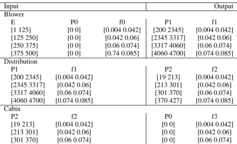
A simple air conditioning system has three components: blower; distribution; and cabin (figure 2).Figure 2 is the model in Mat-lab/Simulink.
Figure 2. A Simplified AC System with 3 Components.
P is pressure, f is airflow rate, E is the electrical power driving the blower. When the blower works, air will pass through the system. We only consider the behavior at a stable point. The right behavior mode is shown in Table 3.
Table 3. qualitative model for AC system
Input Output Blower E P0 f0 P1 f1 [1 125] [0 0] [0.004 0.042] [200 2345] [0.004 0.042] [125 250] [0 0] [0.042 0.06] [2345 3317] [0.042 0.06] [250 375] [0 0] [0.06 0.074] [3317 4060] [0.06 0.074] [375 500] [0 0] [0.74 0.085] [4060 4700] [0.074 0.085] Distribution P1 f1 P2 f2 [200 2345] [0.004 0.042] [19 213] [0.004 0.042] [2345 3317] [0.042 0.06] [213 301] [0.042 0.06] [3317 4060] [0.06 0.074] [301 370] [0.06 0.074] [4060 4700] [0.074 0.085] [370 427] [0.074 0.085] Cabin P2 f2 P0 f3 [19 213] [0.004 0.042] [0 0] [0.004 0.042] [213 301] [0.042 0.06] [0 0] [0.042 0.06] [301 370] [0.06 0.074] [0 0] [0.06 0.074]
We consider two fault modes. One is the lower efficiency of the blower, which causes a change on output flow rate and pressure. Another fault is the leak at distribution, which causes a lower out-put flow rate and pressure at the outout-puts of distribution. For this system, the pressures are measurable, but not the flows. By sim-ulating the fault modes, we get the fault signature as table 4. We have two solutions: {{VS6(P2, [125 250][0 0]), VS7(P2, [250 375][0
0])},{VS6(P2, [125 250][0 0]), VS8(P2, [375 500] [0 0])}}.
Physi-cally they are correspondent to the sensors on P2. The Vo−causeis
E,P0. The discriminable causal scopes are E= {[125 250] [250 375] [375 500]}, P={[0 0]}. We can distinguish faults within these scopes by observing the fault signature.
Some faults are so-called dynamic faults which are detectable only at the dynamic process. It is possible to use our approach for dynamic faults. As in [10], pseudo variables, which are the derivatives of “flow” or “effort” variables (as in bond graph modelling approach), are added to model the dynamic. Treating the pseudo variables as the normal variables, the approach developed here can be used for the dynamic faults. Actually, this demo system is a dynamic system. Due to the length of the paper, the demonstration for the dynamic faults is not covered.
5
CONCLUSION
This paper considers sensor placement based on discriminability analysis at the design stage. The approach we have presented gives us not only the minimal sensor set but also the causal scopes for fault
Table 4. fault signature matrix F1(Blower) F2(Distribution) VS1(P1,[1 125] [0 0]) 0 0 VS2(P1,[125 250] [0 0]) 0 0 VS3(P1,[250 375] [0 0]) 1 0 VS4(P1,[375 500][0 0]) 1 0 VS5(P2,[1 125] [0 0]) 0 0 VS6(P2, [125 250] [0 0]) 0 1 VS7(P2, [250 375] [0 0]) 1 1 VS8(P2, [375 500] [0 0]) 1 1 VS9(P3, [1 125] [0 0]) 0 0 VS10(P3, [125 250] [0 0]) 0 0 VS11(P3, [250 375] [0 0]) 0 0 VS12(P3, [375 500] [0 0]) 0 0
detectability and discriminability. Using the causal scope concept, we can make more precise conclusions on sensor placement. The sensor placement analysis takes place in the simulation environment and is an automatic approach with no structural knowledge needed. This approach is practical for analysis of real world applications.
REFERENCES
[1] Y. Ali and S. Narasimhan, ‘Sensor network design for maxi-mizing reliability of linear processes’, AICheE Journal, 39(5), 820–828, (1993).
[2] Y. Ali and S. Narasimhan, ‘Redundant sensor network de-sign for linear processes’, AICheE Journal, 41(10), 2237–2249, (1995).
[3] J. Cassar and M. Staroswiecki, ‘A structural approach for the design of failure detection and identification systems’, in In
Proc. IFAC, IFIP, IMACS Conference on ’Control of Industrial Systems, pp. 329–334, Belfort, France, (1997).
[4] M-O. Cordier, P. Dague, F. Levy, J. Montmain, M. Staroswiecki, and L. Trave-Massuyes, ‘Conflicts ver-sus analytical redundancy relations’, the special issues of the
IEEE SMC Transactions - Part B on Diagnosis of Complex Systems: Bridging the methodologies of the FDI and DX Communities, (to appear).
[5] M. Luong, D. Maquin, C. Huynh, and Ragot, ‘Observability, redundancy, reliability and integration design of measurement systems’, in Proc. of 2nd IFAC Symposium on Intel.
Com-ponents and Instruments for Control Applications (SICIA’94),
(1994).
[6] F. Madron and V. Veverka, ‘Optimal selection of measuring points in complex plants by linear models’, AICheE Journal,
38(2), 227–236, (1992).
[7] E. Scarl, ‘Sensor placement for diagnosability’, Annuals of
Mathematics and Artificial Intelligence, 11, 493–509, (1994).
[8] P. Struss, B. Rehfus, F. Cascio, L. Console, P. Dague, P. Dubois, Dressler, and D. Millet, ‘Model-based tools for the integra-tion of design and diagnosis into a common process’, in Proc.
of 13th Int. Workshop on Principles of Diagnosis, pp. 25–32,
(2002).
[9] L. Trave-Massuyes, T. Escobe, and R. Milne, ‘Model-based di-agnosability and sensor placement application to a frame 6 gas turbine subsystem’, in Proc. of 12th Int. Workshop on
Princi-ples of Diagnosis, pp. 205–212, Sansicario, Via Lattea, Italy,
(2001).
[10] Y. Yan, ‘Qualitative model abstraction for diagnosis’, in Proc.
of 17th Int. Workshop on Qualitative Reasoning, pp. 171–179,

![Table 4. fault signature matrix F1(Blower) F2(Distribution) VS 1 (P1,[1 125] [0 0]) 0 0 VS 2 (P1,[125 250] [0 0]) 0 0 VS 3 (P1,[250 375] [0 0]) 1 0 VS 4 (P1,[375 500][0 0]) 1 0 VS 5 (P2,[1 125] [0 0]) 0 0 VS 6 (P2, [125 250] [0 0]) 0 1 VS 7 (P2, [250 375]](https://thumb-eu.123doks.com/thumbv2/123doknet/14192435.478353/7.892.83.414.115.322/table-fault-signature-matrix-blower-distribution-vs-vs.webp)
