• Aucun résultat trouvé

Minimum-Cost Virtual Network Function Resilience

N/A
N/A
Protected

Academic year: 2021

Partager "Minimum-Cost Virtual Network Function Resilience"

Copied!
7
0
0

Texte intégral

(1)

HAL Id: hal-02456229

https://hal.archives-ouvertes.fr/hal-02456229

Submitted on 27 Jan 2020

HAL is a multi-disciplinary open access

archive for the deposit and dissemination of

sci-entific research documents, whether they are

pub-lished or not. The documents may come from

teaching and research institutions in France or

abroad, or from public or private research centers.

L’archive ouverte pluridisciplinaire HAL, est

destinée au dépôt et à la diffusion de documents

scientifiques de niveau recherche, publiés ou non,

émanant des établissements d’enseignement et de

recherche français ou étrangers, des laboratoires

publics ou privés.

Minimum-Cost Virtual Network Function Resilience

Yannick Carlinet, Nancy Perrot, Anderson Alves-Tzitas

To cite this version:

Yannick Carlinet, Nancy Perrot, Anderson Alves-Tzitas. Minimum-Cost Virtual Network Function

Resilience. INOC 2019, Jun 2019, Avignon, France. �10.5441/002/inoc.2019.08�. �hal-02456229�

(2)

Minimum-Cost Virtual Network Function Resilience

Yannick Carlinet

Orange Labs Networks

Chatillon, France yannick.carlinet@orange.com

Nancy Perrot

Orange Labs Networks

Chatillon, France nancy.perrot@orange.com

Anderson Alves-Tzitas

Univ. Federal de Minas Gerais

Brazil

andersontzitas02@gmail.com

ABSTRACT

In the future 5G networks, a wide range of new services with strong requirements will be delivered in the form of chains of service functions on independent virtual networks. These virtual networks will be deployed on demand, each one adapted to the specific service requirements. For infrastructure providers a real challenge consists in providing and setting up the required virtual networks (network slices) while guaranteeing strict Service Level Agreements. One of the major stakes is to be able to provide failure protection for the service function chains at minimal cost. In this work, we consider a set of deployed service chains, and we study the best strategy to protect them at minimal cost. We propose mathematical formulations that provide optimal backup functions placement over a network, and the associated backup paths for each VNF of all the chains. We develop an efficient ILP-based heuristic relying on a separation of the problem into smaller ones to solve large scale instances. We show that our heuristic is competitive, both regarding the solution quality and the solving time.

1

INTRODUCTION

1.1

Telecom context

Network operators face the challenge of making their network more flexible and cost-effective. They also have to plan the evo-lution of their networks for the incoming 5G networks. Indeed, some 5G services, such as the Ultra-Reliable Low Latency (URLL), require the network functions to be executed as close as possi-ble to the end-user. This means that the operators will have to split and distribute the network functions over multiple network nodes. Thanks to the maturity of virtualization technologies, Vir-tual Network Functions (VNF) have the capability to run inside Virtual Machines (VM) or containers on commodity hardware. In addition, the concept of Network Slicing will bring even more flexibility, as it allows several virtual networks to run on a unique physical infrastructure, provided by one or several infrastructure providers. This flexibility brings the following benefits:

• On-Demand Network. Network Functions can be deployed and updated remotely, as opposed to manually installing and plugging a hardware equipment to the network. Net-work capacity can also be scaled down or up on-the-fly, depending on the current demand.

• Cost-effectiveness. Maintenance and exploitation of the physical infrastructure are mutualized between the service providers.

• Automatization. Operations on software are easily autom-atized, enabling scaling, healing, reduced delays to market new services, among others.

A Network Slice could be seen as a set of VNFs that are or-ganized into Service Function Chains (SFC), that specifies the

© 2019 Copyright held by the owner/author(s). Published in Proceedings of the International Network Optimization Conference (INOC), June 12-14, 2019: Distribution of this paper is permitted under the terms of the Creative Commons license CC-by-nc-nd 4.0.

sequence of VNFs crossed by the traffic for a specific service. Figure 1 shows an example of a Service Function Chain taken from a use-case defined at IETF (Internet Engineering Task Force) [10]. The provided service is video optimization and it consists of three basic Virtual Network Functions: the Steering Proxy, which is able to redirect HTTP traffic, a DPI-based (Deep Packet Inspector based) controller, which checks for video traffic, and an optimizer, which transcodes the video into a suitable format for the user terminal.

Figure 1: Example of Service Function Chain (SFC). However, this shift in the networking paradigm comes with many technological obstacles to overcome. One of them concerns the resilience of the slices and the associated services.

1.2

Problem Statement

To operate a service, the VNFs of the service chains must be installed in some network nodes, and the traffic routed through the installed VNFs. Some of the VNFs could possibly be shared among several different chains to reduce the exploitation costs, while the capacity limitations and security requirements are met. Figure 2 illustrates a small example of two different SFCs to be routed between an origin-destination pair (1, 6). SFC1 (respec-tively SFC2), in red color (resp. blue color), corresponds to a service that requires the functions VNF1 and VNF3 (resp. VNF1, VNF2 and VNF4). A SFC routing and VNF placement solution is illustrated. VNF1 is installed in node 2 and shared by both SFCs.

Figure 2: Example of deployed Service chains For a commercially exploited network, having a resiliency scheme for each failure scenario is mandatory. Figure 3 illustrates a rerouting scenario of the previous example in case of a failure of the node 2, assuming that a backup of VNF1 has been previously installed on node 3. In this example both SFCs are to be rerouted through the backup node 3.

The aim of this paper is to answer the question of how to make the Service Function Chains resilient to node and link failures. More specifically, the goal is to protect all the Service Function Chains already deployed against a single node or link failure, at minimum cost. It means that all the Virtual Network Functions

(3)

that compose the Service Chains must be protected. We assume that a backup VNF can be used as a backup VNF for several nominal VNFs. Similarly, nominal VNFs with spare capacity can be used as backup VNF. The new routes to the backup VNFs must be disjoint from the corresponding nominal route, to protect from link failure, while satisfying the same latency and capacity constraints as for the nominal path.

Figure 3: Example of node and routing back-up Considering routing and placement of nominal and backup SFCs jointly would yield better solutions, as it would allow a bet-ter usage of network resources. However, in operational settings, realistic scenarios are likely to consider a two-phase deployment.

1.3

State of the Art

In [1], Allybokus et al. consider the problem of VNF placement for the composition of Service Function Chains. Resiliency is taken into account to a certain extent with the addition of anti-affinity rules in the model.

The ETSI (European Telecommunications Standards Institute) has studied the issue of reliability in Network Function Virtual-ization and has given a comprehensive list of features and models for end-to-end reliability [4]. In [6], Hmaity et al. solve the prob-lem of the placement of primary VNFs and backup VNFs, so that the service chains are protected against node and/or link failure. In the end-to-end protection scheme, the backup path does not use any link or node from the primary path. In this scheme, the service chains are resilient against the failure of all the links and all the nodes. In [11], Qu et al. aim at finding the best service chain embedding and routing, for minimizing the overall net-work bandwidth consumption. The problem considers reliability of the service chains with constraints to guarantee that there are enough backup VNF for a given target reliability. In [8], Kong et al. determine the number of VNF replicas required to guarantee the availability of the SFC, and place these replicas on the routing path. In [3], Engelmann and Jukan study the reliability of SFCs with flow parallelism. They evaluate the number of backup VNF necessary to reach a certain service reliability. They also study various placement strategy for the backup VNF. In [13], Wang and Doucette present an algorithm that aims at maximizing the network availability with the approach offered by Shared-Backup Path Protection (SBPP).

We observe that in the cited work, the backup path is disjoint from the working path. In practice, this level of resilience is often too costly and hardly needed since the event of all nodes and all links failing at the same time should seldom occur (if at all). The practical approach for network resiliency is to protect the network operations from a certain number of simultaneous failures. In this paper, we propose and solve a problem that is more relevant to the practical cases of network resiliency design. In addition, our approach is to help network architects to design

a resilient network, in a cost-efficient manner. This is why we seek to minimize the cost of deployment, by contrast to the cited works.

2

THE VIRTUAL NETWORK FUNCTION

RESILIENCE PROBLEM (VNFR)

2.1

Problem Definition

The network is represented by a directed graphG(V , A), where V is the set of network nodes and A the set of arcs. Each network nodeu corresponds to a site in which a network function could be executed, either by running it on existing server or by opening a new site. Opening a new site has a high costmuand corresponds to setting up a new small DC on an eligible site. We assume that the nominal service chains are already deployed in the network. This assumption corresponds to many planned real use-case, in particular when protecting service chains related to critical virtualized functions like vEPC (virtual Evolved Packet Core, [9]) or vRAN (virtual Radio Access Network, [2]). The nominal functions already in place in the network can be shared and used to protect other service chains, and the residual capacityCu ∈ N of used servers can be used to install new functions.

Each arc (uv) of G is characterized by a weight luvthat is a function of the transmission delay between nodesu and v, by a maximal bandwidth capacityBuv, and by a unitary usage cost euv.

The set of all the VNFs to be protected against failure is denoted byF . Each virtual function is characterized by a type f ∈ F , and a maximal flow ratetf the function is able to process. The placement cost of a new function of typef in a node u is denoted hfu.

A service chaink ∈ K is composed of an ordered set of virtual network functions, and an associated routing pathPk. It is char-acterized by a traffic demand between origin-destination nodes, named respectivelyokanddk. Without loss of generality, we de-compose each service chaink into micro chains i, i = 1, . . . , |Fk| composed of one function each, of typefki ∈F .

Then, from now, a section (i, k) corresponds to a unique func-tion between an origin nodeoikand a destination nodedki along the routing pathPkof the global service chain. Then,oikis the node wherefki−1is placed ifi ≥ 2, okotherwise, anddki the node wherefki+1 is placed ifi ≤ n − 1, dk otherwise. The paths of these micro chains are sectionsSki of the pathPk. An example of nominal service chain path is given in Figure 4. The repre-sented SFC is routed along a pathP1 from the source node o1to

the destination oned1, and the flow runs 3 functionsf1i, with

i = 1, 2, 3. The three corresponding sections Si

1, withi = 1, 2, 3

are respectively represented in figures 5, 6 and 7.

Figure 4: A service function chain pathP1, composed of 3

functions

The service chain sections deployed in the network are defined by two set of parameters:

(4)

•puikf that has value 1 is a VNF of typef in section i of service chaink is installed on u, 0 otherwise, and •quvik whose value is 1 if the traffic in sectioni of service

chaink is routed along arc (uv), 0 otherwise.

Figure 5: First section of PathP1,S11

Figure 6: Second section of PathP1,S21

Figure 7: Third section of PathP1,S13

All the notations previously introduced in this section are summarized in Table 1.

2.2

Problem Formulation

The Virtual Network Function Resilience (VNFR) Problem can be formulated as an integer linear program. The four types of decision variables are :

• Routing variables ruvik =


1 if (u,v) is used to re-route section i, k 0 otherwise • Function placement yikfu =       

1 if backup function off for section i of k is placed on nodeu

0 otherwise

• Number of instances of a same type of the backup function f installed on node u

xuf ∈ N • Opening of a new site zu =       

1 if the nodeu is newly used to install at least one back up function

0 otherwise

Then, a compact formulation for the problem is as follows : min Õ u ∈V Õ f ∈F hfuxuf + Õ u ∈V \N muzu+ Õ (uv)∈A Õ k ∈K Õ i ∈Sk euvbkruvik (1) subject to Õ (uv)∈A ruvik − Õ (v′u)∈A rvik′u=          1 ifu = oki − 1 ifu = dki 0 otherwise ∀i ∈ Sk, ∀k ∈ K, ∀u ∈ V . (2) Õ k ∈K Õ i ∈Sk rik uvbk ≤Buv ∀(u, v) ∈ A (3) Õ f ∈F xuf ≤Cu ∀u ∈ V (4) Õ (uv)∈A ruvikluv ≤Lik ∀k ∈ K, ∀i ∈ Sk (5) Õ k ∈K i ∈Sk  bkyuik f − Õ k′∈K \k i ∈Sk′ piku′f(tf −bk′) ≤tfxuf ∀u ∈ V , ∀f ∈ F (6) puik f ≤ Õ u′∈V \u yuik f′ ∀u ∈ V , ∀k ∈ K, ∀f ∈ F, ∀i ∈ Sk (7) rik uv+ qikuv ≤ 1 ∀k ∈ K, ∀(u, v) ∈ A, ∀i ∈ Sk (8) Õ f ∈F xuf ≤Cuzu ∀u ∈ V \N (9) yuik f ≤ Õ (uv)∈A rik uv+ rvuik  ∀u ∈ V , ∀k ∈ K, ∀f ∈ F, ∀i ∈ Sk (10) ruvik ∈ {0, 1} ∀k ∈ K, ∀(u, v) ∈ A, ∀i ∈ Sk yuik f ∈ {0, 1} ∀f ∈ F, ∀k ∈ K, ∀u ∈ V , ∀i ∈ Sk xuf ∈ N ∀f ∈ F, ∀u ∈ V zu ∈ {0, 1} ∀u ∈ V

The objective (1) of the problem consists in minimizing the whole cost of protecting the service chains against a single failure. The first term refers to the installation cost of a functionf in a siteu, the second one to the cost of opening a new site u, and finally the last one refers to the cost of re-routing the traffic of sectioni, of demand k, on the arc (u,v).

The first set of constraints (2) are the flow conservation con-straints, to ensure the flow continuity on the back up routes for all the demands on all the network nodes. The constraints (3) are to ensure that the sum of the flows routed on each arc are less or equal to the bandwidth limit capacity. The constraints (4) are the node capacity constraints and (5) the latency constraints all along the backup routes of all the demands. The maximal flow rates that can be processed by a functionf on a node u is expressed in (6) : the capacity of a function being the capacity of the new installed function instances in addition to the residual capacity of the functionsf already installed for the nominal chains.

The placement constraints (7) are to ensure that each nominal functionf has a back up function installed on another node, while constraints (8) are to ensure the disjunction between nominal and backup paths. The constraints (9) are to define the opening of a site : if at least one functionf is installed on a site u ∈ V \N , ie a site where no function has been installed yet. Finally, constraints (10) are to link the backup functions to the backup routes for all the functions.

2.3

A variant with protection sharing

A shared protection model can easily be obtained from this model, considering that just one VNF failure can occur at a given time, in the same geographical area. The shared protection consists

(5)

Table 1: Indexes, Sets, Constants, and Variables Indexes

f Virtual Network Function types u Nodes

k Service Function Chains i Sections of a service chain (u,v) Arcs

Sets V Set of nodes

A Set of arcs F Set of VNF types

K Set of service chains to protect S Set of all sections of all chains

N Set of open nodes i.e. hosting at least one VNF Constants

Graph notation

Cu Max number of VNF that can be hosted onu mu Cost of opening nodeu

luv Latency of arc (u,v)

Buv Bandwidth capacity of arc (u,v)

euv Cost per traffic unit on arc (u,v)

Service chains Pk Nominal path of service chaink ok Source node for service chaink dk Destination node service chaink bk Bandwidth necessary for service chaink Fk Set of VNFs in service chaink

Sk the set of sections in pathPk

tf Maximum rate off

huf Cost of installingf in node u Service chain sections si

k Source node of the sectioni of service chain k

Sf The set of sections containing functionf

dki Destination node of the sectioni of service chain k ni

k Backup node for backup sectioni of service chain k

fki VNF type in the sectioni of service chain k Lik Max. latency for sectioni of service chain k puikf Binary indicator of nominal VNFs placement

qik

uv Binary indicator of nominal arc usage

in reserving, in each node, a free capacity space to run only the VNF with the largest capacity requirement, so that any single VNF could be run.

Thus, the capacity constraint Equation (6) becomes : max k ∈K i ∈Sk (bkyuikf) ≤tfxuf + Õ k ∈K i ∈Sk Õ k′∈K\k i ∈Sk′ piku′f(tf −bk′) ∀u ∈ V , ∀f ∈ F And the bandwidth constraint (3) becomes :

max

k ∈K i ∈Sk

(bkruvik) ≤Buv ∀(u,v) ∈ A

This alternate formulation is referred to as PS-VNFR (Protec-tion Sharing VNFR) in the following.

Table 2: Compact formulation

|V | |A| |F | |S | Time (s) Var. Constr. 30 198 20 400 1820 319,830 892,258 50 538 40 500 >3600 1,271,050 3,568,138 100 2030 40 400 >3600 2,416,100 6,474,630

2.4

Problem Formulation Analysis

These formulations have been solved to optimality using the commercial solver Cplex 12 ([7]). The largest generated instances, described in section 4.1, couldn’t be solved within one hour. An illustration of the size of the formulation (number of variables and constraints) of VNFR is given in Table 2; where |V | and |A| refers to the graph size, |F | to the number of function types, and |S | is the number VNF instances, i.e. the number of chain sections to be protected against failure. From the formulation of the problem, we can compute the number of variables as

|S ||A| + |S||F ||V | + |F ||V | + |V | (11) and the number of constraints as

|A| + 2|V | + |S| + |V ||S| + 2|F ||V | + 2|S||A| + 3|V ||S||F | (12) We can observe from Equation (11) that for a given graph (i.e. with given V and A), the factor for the number of function types is |V | and the factor for the number of sections is |A|. In typical production networks, the number of arcs is much greater than the number of nodes, i.e. |V | ≪ |A|. The same reasoning applies for the number of constraints, in Equation 12. Therefore, we conclude that the size of the formulation is particularly sensitive to the number of sections, for a given graph.

3

ILP-BASED HEURISTIC

For some instances, solving the ILP (Integer Linear Program) to optimality might not be feasible in a reasonable time. For this reason, we have designed a heuristic called DC-VNFR (Divide and Conquer in the VNFR problem). This heuristic is based on the principle of dividing the original problem into a set of smaller problems. The approach is to process the backups for each type of VNF, one type at a time. More specifically, the set of all the sectionsS is divided into subsets Sf such thatSf contains all the sections that contain a VNF of typef .

The VNFR problem is then solved for eachSf separately. The order of resolution is by decreasingλf, withλf = Í(i,k)∈Sfbk. In other words, we determine the backups for the type of VNF with the largest traffic first.

The heuristic DC-VNFR is detailed in Algorithm 1.

As the heuristic consists in fixing a set of variables at each iteration, it may not find a feasible solution for some instances. In that case, the algorithm stores the rejected backups in a set R and carry on the processing. However, over all our numerical experiments the heuristic has always terminated with a feasible solution.

4

RESULTS

4.1

Random Instances Creation

In order to evaluate the performance of our model, we have designed a random instance generator, that allows us to generate arbitrarily large instances. It is implemented with python3 and the networkX package [12].

(6)

Algorithm 1: The DC-VNFR heuristic

Input : An instance of the VNFR problem (cf. 2), with S = Ðf =1|F | Sf, withSf the set of all sections with function typef

Output : A solution to the VNFR problem (i.e. ¯xuf, ¯yuikf, ¯zu, ¯

ruvik), the total costct, and the set of rejected demandsR

1 Compute all theλf = Í(i,k)∈Sfbkforf ∈ F 2 Sort the setsSf by decreasingλf

3 for f ← 1 to |F | do

4 Solve VNFR to optimality withSf instead ofS 5 if there is a solution then

6 Update variables ¯xuf, ¯ykfu , ¯zu, ¯ruvk 7 Update total costct

8 Update capacities of arcs and nodes 9 for allu such that zu = 1 do 10 N ← N ∪ {u} 11 end 12 else 13 R ← R ∪ {Sf} 14 end 15 end

The inputs for the random instance generator are the number of nodes in the graph, the number of types of VNF and the number of sections. The other parameters are randomly and uniformly chosen in-between an input interval given in Table 3.

The arcs are added as follows. First a path that connects all the nodes is added, so as to ensure that the graph is connected. Then, arcs are chosen randomly and added until a certain percentage of the maximum number of arcs in the graph is reached. In the following, we name the graphs that have 20% of the maximum number of arcs type A and the graphs at 80% type B (cf. Table 3). These values were selected in order to assess the impact of the graph density on performance.

Table 3: Parameters for random instances Intervals Cu [1, 3] luv [1, 20] Buv [100, 500] tf [1000, 2000] bk [1, 20] Lk [100, 500] euv [1, 5] hfu [10, 100] mu [100, 300] Graphs type A 20% complete type B 80% complete

The nominal Service Function Chains are placed as follows: first the origin and destination nodes of each section are randomly selected, then a node is randomly selected on the shortest path to host the VNF. The type of the VNF is also randomly selected.

4.2

Numerical Results

We have generated random instances with varying numbers of nodes and varying number of sections. For a given set of input parameters, we have generated 10 random instances. Then, we have solved all the instances, first with the ILPs (Integer Linear Programs) described in section 2 and then with the DC-VNFR heuristic described in section 3. The ILPs were implemented in Python3 with the Pyomo library [5] and the heuristic was also developed with Python3. We have recorded the execution time in terms of CPU time, and recorded the relative gap between the optimal solution and the solution given by DC-VNFR.

First, it is interesting to note that the two ILPs presented in section 2 yield to the same results (both in terms of objective function and execution time). Therefore, in the following we refer simply to the optimal solution as the ILP. This is due to the fact that, in the random instances we have generated, the parameter tf (maximum rate processed by a function) was high enough not to need to instantiate two of them in a node. In addition, the capacity of the links were not saturated. In consequence, since both constraints (3) and (6) were not saturated, there is no difference with the model that relaxes them. We could check that, on the instances where one or both these constraints were actually saturated, the objective was lower with the PS-VNFR variant.

Figures 8 and 9 show the CPU Time needed for the resolution of the ILP and the execution of the heuristic, when varying re-spectively the number of nodes in the graph and the number of sectionsK. The y-axis scale is logarithmic so it appears from the figures that there is almost always at least an order of magnitude in the performance of the heuristic and the exact resolution.

Figures 10 and 11 represent the relative gap between the DC-VNFR solution and the optimum. The relative gap is defined as (β −α)/α with α the minimum cost and β the cost of the solution provided by DC-VNFR. When varying the number of nodes, the relative gap is always below 0.6%.

4.3

Discussion

The results given in section 4.2 first show that the performance gain with the proposed algorithm over the exact resolution is very good, irrespective of the number of nodes in the graph or the number of sections to protect. It is also noteworthy that the type B instances take more time to solve, in average, than the type A instances. This is because the combinatorial exploration is larger when the graph is more connected.

The results also show that the proposed algorithm yields high-quality solutions, in the sense that whatever the number of nodes in the graph, the gap to optimality stays under 0.6%. In fact, the heuristic is always optimal when the node capacities are not saturated. This is due to the fact that, in that case, the problems of finding the backups for each VNF type are independent from one another. Since in DC-VNFR the optimal solution is found for each VNF type separately, the combined solution remains optimal. We have also observed that when the node capacities are less saturated, the solutions of DC-VNFR tends to be closer to the optimal solutions, which seems quite natural.

However, when varying the number of sections, two opposite trends appear. With type A instances, the gap to optimality in-creases with the number of sections (after 100 sections). This is due to the fact that, for sparse graphs, there is a limited number of nodes to choose from, for the selection of the backup node (because of the latency constraints). In consequence, the node

(7)

Figure 8: CPU Time vs. Number of Nodes

Figure 9: CPU Time vs. Number of Sections

Figure 10: Gap vs. Number of Nodes

Figure 11: Gap vs. Number of Sections

capacities are more often saturated, leading to sub-optimal place-ment of backup VNfs. In contrast, with type B instances, the gap decreases (cf. Figure 11). This is because in that case, there is a larger number of choices for the backup node, which means they are less prone to reach their capacity, which allows the heuristic to lead to a near-optimal solution.

In conclusion, the DC-VNFR heuristic allows to take advantage of the mutualization of the backups of each particular VNF types. It is a good compromise between the optimal resolution of the ILP and a reasonable computation time.

5

CONCLUSION

In this work, we have studied how to improve the resiliency of a set of given Service Function Chains, in a practical and cost-effective manner. The aim is to deploy a backup VNF and an associated backup path for each VNF of all the chains. Since the goal is to protect against a single failure, the backups can be mutualized for several nominal VNFs, and also a nominal VNF with spare capacity can be used as backup. The formulation that we proposed allows to solve this problem at minimal cost, and an ILP-based heuristic, relying on a separation of the problem into smaller ones, is provided in order to solve large scale instances. Empirical results on instances representative of real use-cases show the benefits of this approach.

ACKNOWLEDGMENTS

This work is supported by the french Agence Nationale de la Recherche (ANR), Project MAESTRO-5G ANR-18-CE25-0012.

REFERENCES

[1] Z. Allybokus, N. Perrot, J. Leguay, L. Maggi, and E. Gourdin. 2018. Virtual Function Placement for Service Chaining with Partial Orders and Anti-Affinity Rules. Networks 71 (2018), 97–106.

[2] C. J. Bernardos, A. Rahman, and A. Mourad. 2018. Service Function Chain-ing Use Cases in Fog RAN. Internet-Draft draft-bernardos-sfc-fog-ran-04. Internet Engineering Task Force. https://datatracker.ietf.org/doc/html/ draft-bernardos-sfc-fog-ran-04 Work in Progress.

[3] A. Engelmann and A. Jukan. 2017. A Reliability Study of Parallelized VNF Chaining. CoRR abs/1711.08417 (2017). arXiv:1711.08417 http://arxiv.org/abs/ 1711.08417

[4] ETSI. 2016. Network Functions Virtualisation (NFV) ; Reliability ; Report on Models and Features for End-to-End Reliability. ETSI GS NFV-REL 003 V1.1.2 (2016).

[5] W. E. Hart, C. D. Laird, J.P. Watson, D. L. Woodruff, G. A. Hackebeil, B. L. Nicholson, and J. D. Siirola. 2017. Pyomo–optimization modeling in python (second ed.). Vol. 67. Springer Science & Business Media.

[6] A. Hmaity, M. Savi, F. Musumeci, M. Tornatore, and A. Pattavina. 2016. Virtual Network Function placement for resilient Service Chain provisioning. 2016 8th International Workshop on Resilient Networks Design and Modeling (RNDM) (2016), 245–252.

[7] IBM ILOG. 2015. IBM ILOG CPLEX V12.6: User’s manual for CPLEX. [8] J. Kong, I. Kim, X. Wang, Q. Zhang, H. C. Cankaya, W. Xie, T. Ikeuchi, and

J. P. Jue. 2017. Guaranteed-Availability Network Function Virtualization with Network Protection and VNF Replication. GLOBECOM 2017 - 2017 IEEE Global Communications Conference (2017), 1–6.

[9] S. Matsushima and R. Wakikawa. 2016. Stateless user-plane architecture for virtualized EPC (vEPC). Internet-Draft draft-matsushima-stateless-uplane-vepc-06. Internet Engineering Task Force. https://datatracker.ietf.org/doc/ html/draft-matsushima-stateless-uplane-vepc-06 Work in Progress. [10] J. Napper, M. Stiemerling, D. Lopez, and J. Uttaro. 2018. Service Function

Chaining Use Cases in Mobile Networks. Internet-Draft draft-ietf-sfc-use-case-mobility-08. Internet Engineering Task Force. https://datatracker.ietf.org/doc/ html/draft-ietf-sfc-use-case-mobility-08 Work in Progress.

[11] L. Qu, C. M. Assi, K. B. Shaban, and M. J. Khabbaz. 2017. A Reliability-Aware Network Service Chain Provisioning With Delay Guarantees in NFV-Enabled Enterprise Datacenter Networks. IEEE Transactions on Network and Service Management 14 (2017), 554–568.

[12] D. A. Schult. 2008. Exploring network structure, dynamics, and function using NetworkX. In In Proceedings of the 7th Python in Science Conference (SciPy. 11–15.

[13] W. Wang and J. Doucette. 2018. Availability optimization in shared-backup path protected networks. IEEE/OSA Journal of Optical Communications and Networking 10, 5 (May 2018), 451–460. https://doi.org/10.1364/JOCN.10.000451

Figure

Figure 1 shows an example of a Service Function Chain taken from a use-case defined at IETF (Internet Engineering Task Force) [10]
Figure 3: Example of node and routing back-up
Figure 6: Second section of Path P 1 , S 2 1
Table 3: Parameters for random instances
+2

Références

Documents relatifs

Traversal time (lower graph) and transmission coefficient (upper graph) versus the size of the wavepacket for three different values ofthe central wavenumber, k = 81r/80 (dashed

A rough analysis sug- gests first to estimate the level sets of the probability density f (Polonik [16], Tsybakov [18], Cadre [3]), and then to evaluate the number of

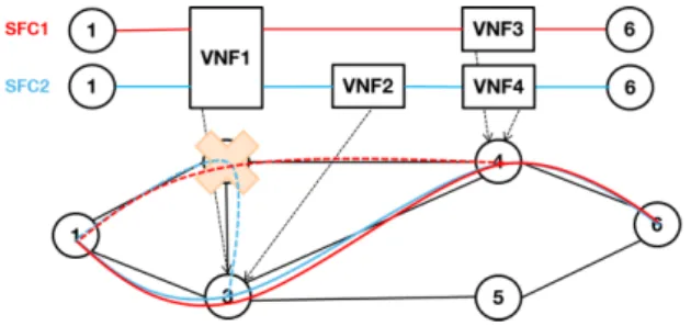
Given the matrix of cost functions and the agents’ demands, one must firstly find a cost-minimizing network (efficiency) and secondly share the cost of this optimal

Fleischner and Stiebitz [3] proved that in every ( Cycle and triangles' graph there is an odd number of Eulerian orientations. They used this result and the 'Graph polynomial

Unit´e de recherche INRIA Rennes, Irisa, Campus universitaire de Beaulieu, 35042 RENNES Cedex Unit´e de recherche INRIA Rhˆone-Alpes, 655, avenue de l’Europe, 38330 MONTBONNOT ST

Explicit examples of linear sized graphs that are Ramsey with respect to T s H are given by the Ramanujan graphs of Lubotzky, Phillips and Sarnak [22] and Margulis [23].. Let us

Toute utili- sation commerciale ou impression systématique est constitutive d’une infraction pénale.. Toute copie ou impression de ce fichier doit conte- nir la présente mention

The basic idea is to form a rough skeleton of the level set L(t) using any preliminary estimator of f , and to count the number of connected components of the resulting