Characterization of Kenyan obsidian through analysis of magnetic properties

Characterization of Kenyan Obsidian Through Analysis of

Magnetic Properties

By

Elizabeth A. Krueger

Submitted to the Department of Materials Science and Engineering in Partial Fulfillment of the Requirements for the Degree of

ARC00E

Bachelor of Science in Archaeology and Materials

at the OF TECHNOLOGY

Massachusetts Institute of Technology _{JUN 0 4 2014}

June 2014

L LIBRARIES @2014 Elizabeth A. Krueger. All rights reserved.

The author hereby grants MIT permission to reproduce and to distribute publicly paper and electronic copies of this thesis document

in whole or in part in any medium now known or hereafter created.

Signature redacted

Signature of Author:

Signatre redacted

Departme4of Materials SciencI and Engineering

Signature redacted

May 2, 2014

Certified by: _I

Certified by:

Accepted by:

Dr. Harry V. Merrick

Lecturer in Archaeology

Thesis Supervisor

Signature redacted

Associate Professor of Materials Science and Engineering

Thesis Supervisor

Signature redacted

V

I

V/Jeffrey C. Grossman

Professor of Materials Science and Engineering

Undergraduate Committee Chairman

Characterization of Kenyan Obsidian Through Analysis of

Magnetic Properties

By

Elizabeth A. Krueger

Submitted to the Department of Materials Science and Engineering on

May 2, 2014 in Partial Fulfillment of the Requirements for the Degree of

Bachelor of Science in Archaeology and Materials

Abstract

Obsidian is known to have been used for tool making in Kenya since the Early Stone Age, appearing as early as 974 thousand years ago (Durkee and Brown, in press). Past research has shown that the study of obsidian artifacts, and the determination of their provenance, can be very useful in reconstructing past civilizations and analyzing the spread of technology and trade. A number of different analytical techniques have previously been utilized to characterize obsidian sources for such studies, including magnetic analysis. This thesis reports the results of a preliminary study to explore the potential of utilizing magnetic analysis for the characterization of obsidian sources in Kenya. A total of 192 samples from 23 localities, belonging to

6 broadly defined petrologically distinct source groups, were analyzed using a

vibrating sample magnetometer to test saturation magnetization (Ms), remanence magnetization (Mr), and coercivity (Hc). Comparing the ratio of Mr/Ms with Hc allowed clear differentiation among three of the analyzed obsidian sources (Groups 14, 19, and 29 from Merrick and Brown 1984a). The magnetic signatures reveal clues about the microscopic Fe mineral grains present in the samples, suggesting that magnetic characterization also has the potential to provide additional value as a supplementary technique to chemical analysis. Based on these preliminary results, it is proposed that future studies could examine the temperature dependence of the magnetic properties of obsidian to provide more complete characterization of the obsidian sources.

Thesis Supervisor: Harry V. Merrick Title: Lecturer in Archaeology

Thesis Supervisor: Geoffrey S.D. Beach

Table of Contents

TITLE PAGE AND SIGNATURES ₁

ABSTRACT 2 TABLE OF CONTENTS 3 LIST OF FIGURES ₄ LIST OF TABLES ₄ INTRODUCTION 5 ARCHAEOLOGICAL PROVENANCE ₅ OBSIDIAN 6

EVOLUTION OF OBSIDIAN PROVENANCE STUDIES 9

KENYAN OBSIDIAN 14

MATERIALS AND METHODS 16

TYPES OF MAGNETISM ₁₆

SAMPLES AND SAMPLE PREPARATION 21

ANALYSIS METHODS ₂₆

RESULTS 28

CHARACTERIZATION BY SQUARENESS AND COERCIVITY 30

SATURATION MOMENT AND FE PERCENTAGE CALCULATIONS 31

PRECISION CALCULATIONS 33

DISCUSSION AND CONCLUSIONS 34

CONCLUSIONS 34

LIMITATIONS 35

POTENTIAL FUTURE WORK 35

ACKNOWLEDGEMENTS ₃₇

APPENDIX A ₃₈

Figure 1. Figure 2. Figure 3. Figure 4. Figure 5. Figure 6. Figure 7. Figure 8. Figure 9. Figure 10. Figure 11. Figure 12.

Initial and Saturation magnetization of Sardinian obsidians,

from M cDougall et al. 1983 ... 12

Generic hysteresis loops and diagrams of the atomic basis for various types of magnetic response... 16

Generic hysteresis loop diagram, measuring applied field (H) against induced magnetic response (M)... 19

M ap of all source localities ... 22

Closer view of source localities map showing group 29 and 32 localities (Merrick and Brown, 1984a)... 23

Photograph of an obsidian specimen... 24

Vibrating sample magnetometer schematic diagram... 26

Sample of visual VSM output from a Baixia Estate sample ... 28

Sample of visual VSM output from a Sonanchi Crater sample... 29

Plot of the coercivity (Hc) versus the hysteretic squareness (Sq)... 30

Plot of saturation moment (Ms) per gram of Fe in the sa m p le ... 3 1 Plot of calculated approximate percentage of Fe in a-Fe203 form in the sam ple... 32

List of Tables

Appendix A. Table 1. Magnetic analysis data from all samples ... 38

Introduction

The goal of this thesis project was to explore the possibility of using magnetic properties as a characterization metric for the study of obsidian provenance in Kenya. This research will add to the available database of general knowledge about magnetic obsidian sourcing in various regions worldwide. No previous magnetic obsidian provenance studies have been conducted in eastern Africa (Coleman,

2008). Three major magnetic properties, discussed in more detail later, were

analyzed here to determine whether any combination of them showed enough patterning to provide useful characterization metrics for sourcing Kenyan archaeological obsidian artifacts.

Archaeological Provenance

Provenance studies, also known as sourcing studies, are a type of archaeological research where various material sources (stone, metal ores, clays, etc.) in a region are characterized using one or more testing metrics to create a sort of "fingerprint" (Cann and Renfrew, 1964) allowing archaeologists to locate the original material sources of archaeological artifacts. Such studies have been shown to be extremely useful in the study of the human past (Glascock et al., 1998).

Tracing artifacts back to the locations where the material itself originated can provide useful information about how ancient societies functioned. Tracing materials found at artifact production sites can give us a look at production

the raw material long distances back to the production site. Artifacts found in other contexts can have important implications regarding early human movement and material exchange patterns, as well as potentially hinting at the material's cultural significance (Glascock et al., 1998).

The provenance postulate states that in order to successfully source an artifact, there must be "a demonstrable set of physical, chemical, or mineral characteristics in the raw material source deposits that is retained in the final artifact" (Rapp and Hill, 2006; 222). This condition allows the comparison of the properties of the artifact with those of various source samples so that the artifact can be matched to its source. There are a number of methods that archaeologists have at their disposal with which to do this. The most common methods in use today for the analysis of obsidians involve the testing of their physical and geochemical properties, either alone or in combination, and comparing them to those of the various obsidian sources in the surrounding area (Rapp and Hill, 2006).

Obsidian

Obsidian is a volcanic silicate glass, which occurs in several forms within pyroclastic deposits (flows, welded layers, and lapilli). It exhibits a strong pattern of conchoidal fracture, which makes it an ideal material for the manufacture of sharp-bladed objects such as cutting tools and spear points. Obsidian is often known for its shiny black color, although it also comes in a variety of other color variants (Miller, 2014). Since the obsidian is liquid before the eruption, thorough mixing usually occurs within the magma chamber, and an entire eruptive event will produce obsidian with

approximately identical chemical makeup. This homogeneity can lead to obsidians with such similar chemistry many miles/kilometers apart depending on the size of the flow.

All obsidians contain trace amounts of various minerals in sub-millimeter sized

crystal grains. The most common mineral found as micro-inclusions in obsidian is magnetite (Fe30 4), which causes obsidian's typical black coloration. Hematite, ilmenite, feldspars, and other minerals are also common (Frahm and Feinberg,

2013). The concentrations, compositions, morphologies, and the size and spatial

arrangement of these mineral grains can all affect the magnetic properties of obsidian. Unlike the bulk chemical composition of the obsidian, the magnetic properties of the mineral grains are affected by the local flow conditions under which the obsidian cooled, which can vary across a single flow, causing intra-flow spatial patterning of the magnetic properties of obsidian (Frahm and Feinberg,

2013).

Obsidian has been the frequent subject of provenance studies in many areas of the world -- including the Near East (Binder et al., 2011), the Mediterranean (Stewart et al., 2003), western North America (Frahm and Feinberg, 2013), Japan (Hall and Kimura, 2002), New Zealand (Sheppard et al., 2011), Mexico (Urrutia-Fucugauchi,

1999), the Andean region of South America (Vasquez et al., 2001), and Kenya

(Brown et al., 2013) -- for a number of reasons. First, it was frequently used in artifact manufacture in ancient times around the world practically everywhere it

was available as a natural resource to ancient peoples (Merrick and Brown, 1984a). Second, obsidian-containing localities tend to be very discretized due to the geologic processes that form them (Carmichael, 2014). Obsidian often gets buried under other layers of rock over time, so it is available on the surface only where it has either been freshly laid down by volcanic activity, or where geologic processes such as erosion have brought older layers to the surface (Miller, 2014). The reemergence of old obsidian layers can lead to the existence of a number of discrete obsidian collection localities within a single obsidian flow. Another reason that obsidian is more conducive to provenance studies than some other materials is that the artifact

forming processes -- e.g. knapping or flaking -- do not affect obsidian in ways that

would affect the properties that are generally used for sourcing materials (Rapp and Hill, 2006). For example: unlike metal ores, which are refined by melting to separate the metal from the unwanted parts of the ore, obsidian artifacts are formed by

processes which do not affect the chemistry or magnetic properties of the original material.

One challenging bit of terminology encountered in archaeological provenance studies is the term "obsidian source". Over the history of obsidian provenance studies, different researchers have used varying definitions of an obsidian "source". It seems that each author's definition has generally been defined by the scale of resolution on which the characterization techniques they used can effectively

differentiate various obsidians. Many previous authors have used the term "source" to mean one chemically "identical" set of localities, presumed to be from the same

eruptive event or flow due to their chemical similarity (e.g. McDougall et al., 1983; Urrutia-Fucugauchi, 1999; Duttine et al., 2008; etc.). This definition is adopted here, as this is the scale of characterization that is mainly being considered here, and different usages of the term "sources" will be identified by alternative descriptive names to differentiate them. One particular example of a usage of "source" in a more geographically restrictive sense occurs in the recent Frahm and Feinberg paper

(2013), where the term "source" refers to the individual quarry localities rather

than clusters of quarries showing similar material properties. In this study the term "locality" will be used to discuss the particular quarry from which an artifact

originated. In addition, what is referred to in this study as a "source" has been referred to as a "source group" or "petrological group" in previous published research done on these samples (Merrick and Brown, 1984a; Merrick and Brown,

1984b; Merrick, Brown and Nash, 1994; Brown et al., 2013). In this study, "source

group" "group" and "source" are used approximately interchangeably.

Evolution of Obsidian Provenance Studies

The development and use of obsidian provenance studies has been a major archaeological success story. Over the roughly fifty years or so that obsidian sourcing has been developing, hundreds of such studies have been conducted (Frahm and Feinberg, 2013). Of the methods that have been tested for sourcing obsidian, chemical analysis techniques - such as spectrometry based methods including optical emission spectrometry (OES) (e.g. Cann and Renfrew, 1964) and more refined inductively coupled plasma mass spectrometry (ICP-MS) (Binder et al., 2011), x-ray fluorescence (XRF) (e.g. Ndiema et al., 2011), electron microprobe

analysis (EMP) (Brown et al., 2013), and neutron activation analysis (NAA) (Hallam et al., 1976) - have come to be widely used and are considered the most successful, although a number of other metrics have also been used at various times to

characterize obsidian sources (e.g. Binder et al., 2011; Duttine et al., 2008; Game in Leakey, 1945). In the case of eastern Africa, alternate sourcing metrics that have been used include refractive index and specific gravity (Game in Leakey, 1945; Walsh and Powys, 1970). Because of its success, chemical composition analysis is the most common obsidian characterization method in use today.

The success of chemical analysis as the leading method of obsidian characterization is in part due to the chemical homogeneity of obsidian within a single flow. Since the obsidian produced from a single eruptive event originated from a single source or chamber of liquid magma, an entire flow will have a homogenous chemical

composition. A single volcano can produce multiple eruptive events over its lifetime, each of which will have similar but not identical chemistries because lighter

elements tend to become depleted in successive eruptions. In theory, chemical analysis could be used to differentiate among flows from the same volcano if enough elements were analyzed. However, it would be impractical to perform such tests for cost reasons and because at some point the chemical variations may be less than the analytical precision of the measurements. In cases of chemically similar flows from successive eruptions of a single volcano, it is often possible to characterize the individual flows using obsidian dating methods (e.g. Bigazzi et al., 1997) or other supplementary techniques.

In the earlier days of obsidian sourcing, chemical analysis methods - typically OES (Cann and Renfrew, 1964), XRF or NAA -- were costly and more time-consuming than other non-chemical methods that were available at the time. These drawbacks made chemical analysis impractical for sourcing large collections of artifacts. These earlier chemical analytical techniques were generally also destructive of the

samples, which is obviously undesirable when it comes to working with scarce archaeological materials. These disadvantages led researchers to search for alternative and perhaps better methods for sourcing obsidian. One of the more commonly studied alternatives to chemical analysis was magnetic testing (McDougall et al., 1983).

The first major magnetic obsidian provenance study was conducted by McDougall (McDougall, 1978; McDougall et al., 1983). The purpose of the study was to examine whether magnetic analysis could be used as an effective alternative to slower and more expensive chemical analysis methods. McDougall and others (1983) analyzed a collection of Mediterranean obsidians consisting of both geological and

archaeological samples. Their archaeological samples had already been chemically analyzed by NAA, and they used this previous chemical sourcing data for

comparison to test the reliability of their magnetic data (McDougall, 1978). They tested a number of magnetic parameters including natural remanent magnetization, saturation magnetization, and mass susceptibility -- another magnetic property that has been used for previous magnetic studies (e.g. Schmidbauer et al., 1986) but is

not further discussed here. Using a combination of these parameters, they were able to partially characterize the obsidian sources in the Mediterranean. However,

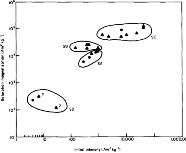
McDougall and others' magnetic data showed high intra-source variability, making the precise characterization of sources more difficult (McDougall et al. 1983). Most of the obsidian sources that had been previously identified through chemical analysis were distinguishable with minimal overlap, but there were a few sources that had too much overlap to be easily distinguishable. This can be seen in Figure 1.

105' 0% E 0 E C 104 102 10LI _{I0 100 10,000 1,000,000}

Initial intensity (Am 2 kq~1)

Figure 1. Initial and Saturation magnetization of Sardinian obsidians, from McDougall et al., 1983. Circles represent source samples, and triangles represent archaeological artifacts. SA, SB, SC, and SD are chemically distinct obsidian sub-types. SC and SD can be clearly

distinguished, but SA and SB are close enough together that distinguishing between the two using this method would not be feasible.

SC

??

A? SD

10-Since McDougall and others' initial study, several other magnetic obsidian provenance studies have been conducted in various regions, including Mexico (Urrutia-Fucugauchi, 1999), and the Near East (Hillis et al., 2010; Frahm and Feinberg, 2013). These studies have generally yielded mixed results, with most finding that magnetic analysis could work in specific cases, but that it is still less reliable than chemical sourcing techniques, and thus not a good substitute. Prior to the current research, no such magnetic studies had been conducted on Kenyan or other eastern African samples.

Magnetic properties, unlike chemical composition, are dependent on the

microstructure and molecular organization of the material (Carmichael, 2014). Since these both depend on the conditions in which the obsidian cooled, the

magnetic properties of obsidian are not always constant across a single flow (Frahm and Feinberg, 2013). This variation can make it difficult to differentiate between obsidian flows using magnetic properties in regions with chemically similar

obsidian sources, like those observed in the studies reference above. Since there is higher intra-source variation in magnetic properties, it is easier for different sources' magnetic signatures to overlap than for their chemical compositions to do

so.

Despite the mixed success of previous magnetic obsidian provenance studies, certain characteristics of eastern African obsidians make them a potential target for better results from magnetic study. The obsidian flows in Kenya are known for

having a much higher range of iron contents than obsidians in most other regions, and given the highly magnetic nature of iron minerals, this wider range may possibly translate to wider inter-source variation, potentially making magnetic sourcing more effective in this region than previous research in other regions has found it to be. Despite improvements in chemical analysis methods, magnetic analysis is still fairly easy and cheap, so if it were useful in discriminating between sources, it might still provide a reasonable alternative to chemical analysis.

Kenyan Obsidian

Obsidian provenance study in Kenya began in the 1940s with P.M. Game's study of the refractive index and specific gravity of obsidian artifacts from the Hyrax Hill archaeological site being studied by Mary D. Leakey (1945). The refractive index is a measure of how light bends across the boundary between different materials, and specific gravity compares the density of a sample to the density of a reference substance, usually water, under the same conditions. Game compared the data from these archaeological samples to data from samples from the Njorowa Gorge and Mt.

Eburru obsidian sources. From this comparison, he was able to determine that ancient people had been using obsidian from both of these sources (Game in Leakey, M.D. 1945).

Chemical analysis as a method for obsidian provenance was not used in Kenya until the 1970's and 1980's. The first of such studies in the region (Michels et al., 1983; Merrick and Brown, 1984a; Merrick and Brown, 1984b) utilized atomic absorption spectroscopy (AAS), XRF and electron microprobe analysis (EMP) techniques to

characterize obsidian samples. These techniques proved successful, and they continue to be used to this day. NAA has also been used recently in this region. Coleman and others (2008) showed NAA to have better resolved data clusters than XRF. As of today, more than 80 chemically distinct Kenyan obsidian sources have been characterized, although only about 20 of these are known to have been used archaeologically, and even fewer saw regular use (Brown et al. 2013).

Obsidian artifacts are known to have been in use in Kenya as early as 974,000 years ago (Durkee and Brown, in press). Thereafter, obsidian continued to be used, though uncommonly, throughout the Acheulean period, or the latter half of the Early Stone Age until about 200,000 years ago. Obsidian use in the region picks up in the Middle Stone Age beginning within the last 150,000 years, with the majority of

archaeological sites within a radius of about 50 km from a source of obsidian showing use of it. The first appreciable quantities of obsidian (20% or greater) at sites more distant than 50 km from any obsidian sources also start to appear during this period. By the Late Stone Age, almost all sites in the central Rift Valley in Kenya display considerable percentages of obsidian artifacts, suggesting pervasive

adoption of obsidian as a tool-making material (Merrick, Brown and Nash, 1994).

The Pastoral Neolithic period began in eastern Africa around 2000 BC. In this period, obsidian starts to appear as the dominant material (>90%) in nearly all archaeological sites within 50 km of an obsidian source. Obsidian also begins to be used very frequently further away from sources during this period, with a number

of sites as far as 100-200 km away showing high frequencies of obsidian (Merrick and Brown, 1984a).

Materials and Methods

Types of Magnetism

The magnetic properties of materials are derived from the atomic magnetic

moments of their constituent atoms. Although most people only think of "magnetic" materials as materials that can be permanently magnetized, many materials

generate some kind of response to being placed in a magnetic field (Borradaile et al.,

1998). Some of the common types of magnetic response are shown in Figure 2,

along with relevant examples of materials that produce each kind of response.

Paramagnetic Ferromagnetic Antiferromagnetic Ferrimagnetic

M M M M

H H H H

-r

)ks

l0

00e

Ex: Aluminum Ex: Pure Fe metal Ex: FeO, a-Fe203 Ex: y-Fe2O, Fe304

Figure 2. Generic hysteresis loops and diagrams of the atomic basis for various types of magnetic response.

Paramagnetic

Paramagnetic materials have unpaired electrons, each of which has a fluctuating magnetic dipole moment, but there is no interaction between the electrons of adjacent atoms. The lack of interaction means that the moments are randomly directed, causing a lack of macroscopic magnetization when not under the influence of an external magnetic field. However, when a magnetic field is applied, the

moments will rotate to line up with the direction of the applied field. The strength of this response increases linearly with the strength of the field applied, but quickly

dissipates when the field is removed (Carmichael, 2014).

Ferromagnetic

Ferromagnetic materials are the type of material that most people associate with the concept of magnetism because ferromagnets can hold a strong permanent

magnetic charge. When there is no magnetic field being applied, the exchange

interactions between the individual magnetic dipole moments cause them to line up. The combination of all of the atomic moments is strong enough to cause the bulk

material to have a macroscopic magnetization (Carmichael, 2014).

Antiferromagnetic

Antiferromagnetic materials are similar to ferromagnetic materials in that all of their atomic magnetic moments want to align when there is no applied magnetic field. However, the structure of the material is such that it is favorable for every other atom in the structure to be aligned in the opposite direction, causing the net

magnetic moment of the bulk material to vanish. Thus, although the atomic

moments in an antiferromagnet are aligned, and hence the material is magnetically ordered, it exhibits zero macroscopic magnetization in zero applied field. When an

external magnetic field is applied, antiferromagnetic materials act similarly to paramagnetic materials, with the dipole moments rotating towards the same

orientation (Carmichael, 2014).

Ferrimagnetic

Ferrimagnetic materials, like antiferromagnetic materials, have adjacent atoms that align in opposite directions. However, the strength of the magnetic moment on adjacent atoms is not equal, so ferrimagnets can still have a non-zero net magnetic moment in the absence of an applied magnetic field (Carmichael, 2014).

The bulk magnetic properties of rocks come from the magnetic properties of the constituent mineral grains (Carmichael, 2014). In general, only a small fraction of these mineral grains are magnetic materials. In obsidian, various iron oxides make

up the majority of the magnetic mineral grains. Examples of the most relevant Fe oxide variants are listed in Figure 2, and are typically either antiferromagnetic (FeO, a-Fe203) or ferrimagnetic (y-Fe203, and Fe304).

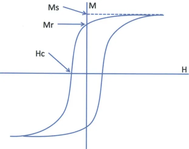
The graph in Figure 3 shows a generic example of a hysteresis loop. A hysteresis loop measures the reaction of a material to being put in a magnetic field, plotting the material's induced magnetization (M) in response to an applied field of varying strength (H). The applied field is cycled, first increasing in strength in one direction

Ms

Mr

Hc

M

H

Figure 3. Generic hysteresis loop diagram, measuring applied field (H) against induced magnetic response (M). The points at which saturation magnetization (Ms), remanence magnetization (Mr), and coercivity (Hc) are measured are labeled.

until the sample's magnetization is saturated and the induced magnetization no longer increases, and then returning to zero and increasing in the opposite direction until the sample has reached its saturation magnetization in the other direction before returning to a state of no applied field (Nave, 2014). This cycling yields a somewhat S-shaped loop, although the exact shape of the curve can vary depending on what type of magnetic response the material produces (see Figure 2).

Several magnetic properties can be determined from a hysteresis loop test. The parameters studied here are saturation magnetization (Ms), remanent

magnetization (Mr), and coercivity (Hc). Figure 3 shows where each of these properties appears on a hysteresis loop diagram. Saturation magnetization is the maximum induced magnetization that can be achieved. Remanent magnetization is the strength of the induced magnetization when the applied field drops to zero, showing how strong the magnetization on the sample is when it is no longer in a magnetic field. Coercivity is the strength of the applied magnetic field required to reduce the sample's induced magnetization to zero, measuring how strong a magnetic field is required to demagnetize the sample (Nave, 2014).

Magnetic analysis measures properties of the sub-millimeter-scale magnetic mineral grains in the obsidian. In the process of cooling, obsidian undergoes a range of temperatures and viscosities, as well as deformation and oxidation, all of which

affect the size and composition of the mineral grains present in the obsidian (Miller, 2014). These variables can differ widely within a single obsidian flow, causing variation in magnetic properties across the flow. This interpretation sees support in previous studies that show large variability in magnetic properties across a given flow (Urrutia-Fucugauchi, 1999; Frahm and Feinberg, 2013).

Since the magnetic properties of obsidian depend on the chemical phase and microstructure of the Fe oxide grains, these properties can potentially be used to discriminate between obsidians formed under different conditions. Determining the forms of Fe present could provide an additional discriminant for magnetic

chemical analysis. Such methods can provide information that even very precise chemical analysis cannot. For example, the two main forms of Fe203 that are present in obsidian (cc-Fe203 and y-Fe203) would be indistinguishable from chemical tests due to the fact that both forms have identical chemical composition. However,

a-Fe203 is antiferromagnetic, while y-a-Fe203 is ferrimagnetic, so the two should show very different magnetic responses, allowing discrimination between them

(Carmichael, 2014). While the tests performed here cannot completely determine the forms of Fe oxides present in the samples, comparing the weight-normalized Ms to the weight percent of Fe in the obsidian sample can give some information on the fraction of Fe in various forms, discussed further in the Results section.

Samples and Sample Preparation

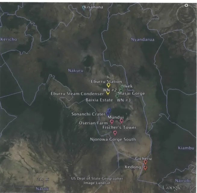
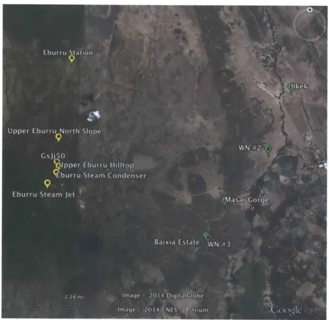
This study analyzed specimens from the obsidian collection from Harry Merrick and Francis Brown's chemical composition sourcing work in eastern Africa (Merrick and Brown, 1984a; Brown et al., 2013). A map of the localities from which the specimens were originally collected is shown in Figure 4. Figure 5 gives a closer view of the central area of the previous map to more clearly show the closely clustered localities in that area. Detailed chemical composition information for all of the samples

analyzed here is available in Brown et al., 2013. This data set was compared with the magnetic data acquired in this study to determine whether magnetic testing could be used as an alternative or accessory technique to supplement

The available Merrick and Brown sample collection included specimens from 23 of the geochemically distinct source groups in Kenya recognized in Merrick and Brown, 1984a. Sixteen of these groups are known to have been used

archaeologically, with only 5-6 of these seeing frequent usage. Of this collection, a total of 192 samples from 26 different pieces of obsidian were analyzed. These pieces were collected from 23 different localities assigned to 6 different petrological

Figure 4. Map of all source localities. Symbol color indicates the petrological group of the locality (Merrick and Brown, 1984a). Pink: Group 20, Red: 14, Yellow: 29, Green: 32, Blue: 8, Purple: 19.

groups (Groups 8, 14, 19, 20, 29, and 32) as recognized by Merrick and Brown (1984a). Only obsidian source groups that have been observed to have been used for artifact manufacture in the past were selected for analysis in this study. The first four groups analyzed (8, 14, 19, and 29) were selected to represent a wide range of Fe contents, as measured by Brown and others (2013). The other analyzed groups (20, and 32) were chosen for their known use as common obsidian sources in

Figure 5. _{Closer view of source localities map showing group 29 and 32 localities (Merrick and}

prehistoric times. A list of samples, their petrological groups and locations, Fe contents, and all collected analytical data are given in Appendix A: Table 1.

To prepare the samples for testing, small chips were flaked off of the specimens with a small copper rod. The chips were then further ground down by hand with the

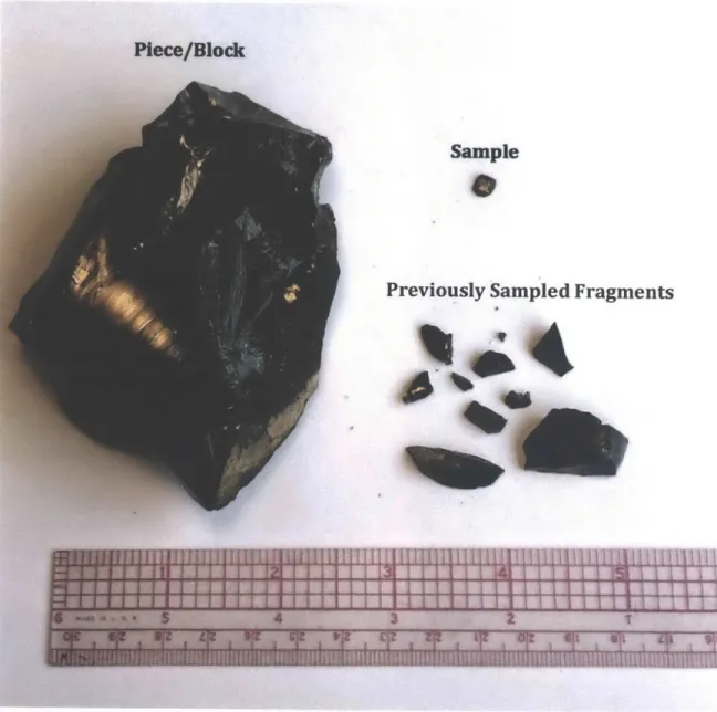
Sample

Previously Sampled Fragments

Figure 6. Photograph of an obsidian specimen, shows examples of how large pieces/blocks and samples are. The photographed material makes up a single specimen, although some specimens contain multiple pieces/blocks. Ruler for scale.

same copper rod to the point where they were approximately the same size (see Figure 6 for scale). Some variation was to be expected considering the fact that the samples were sized by hand and the similarity between sample sizes was

determined by a rough visual estimate. All samples' sizes were compared to the first sample created to establish a consistent approximate size. Although this method does not provide a perfectly consistent sample size, this technique is similar to that used for sample preparation in the recent magnetic obsidian sourcing study by Frahm and Feinberg (2013; sample preparation discussed in Frahm, 2010), one of only two papers located that went into detail about their sample preparation methods. The other paper was the McDougall et al. (1983) paper, which used a different enough magnetometer setup that their sample preparation procedure is not relevant here. Despite the slight sample size variation, initial tests of several samples from the same obsidian specimen suggest that size does not noticeably affect the relevant magnetic parameters once they have been weight-normalized, as was expected.

Most of the specimens available for sampling were single pieces of obsidian, along with some small fragments that had resulted from previous sampling of the pieces (see Figure 6). A few of the potential samples consisted of multiple main pieces, which were collected at the same location and thus considered part of the same petrological group for sampling purposes. In such cases, this study considered each of the larger pieces as a separate "block" to avoid the possibility of unexplained bimodality in the case that the two blocks had significantly different properties.

Analysis Methods

Hysteresis loop data can be collected on a vibrating sample magnetometer (VSM). As shown in Figure 7, a VSM consists of several magnetic coils and a sample holder that is vibrated between them. The field coils create a magnetic field around the

sample, which induces a magnetic moment in the sample. The sample is vibrated up and down, which rapidly changes the magnetic flux felt by the pickup coils. The changing magnetic flux causes a voltage difference across the pickup coils which is directly related to the strength of the induced magnetic moment on the sample. The voltage difference can thus be measured and from that the induced magnetic

moment can be calculated.

sample Field

driver

coils

Vibrating sample

F]

magnetometer

pole

(VSM) pieces

Pickup coils _{sample Yoke}

Electromagnet

Figure 7. Vibrating sample magnetometer schematic diagram. From MIT 3.014 lab handout "Work Derived from Magnetic Hysteresis Curves", Fall 2008.

The samples in this study were analyzed using a Digital Measurement Systems VSM maintained by the MIT Department of Material Science and Engineering in the undergraduate teaching lab. The applied and induced magnetic fields were measured to create a hysteresis loop, from which the Ms, Mr, and Hc were

and then averaged to minimize possible orientation effects or machine calibration errors. All of the tests were performed at room temperature.

Data analysis was performed using a combination of Microsoft Excel and

Mathematica. The final plots were generated using Excel. The magnetic properties mentioned above were analyzed to determine whether any of them, alone or in combination, could be used as an alternate or supplementary method for

differentiating between Kenyan obsidian sources. The potential for characterization was analyzed both between sources and, for the few sources with samples from multiple localities, between localities within the same source.

In addition to the above data comparison, an approximation of the forms of Fe present in the samples was also calculated. For the purposes of these calculations, it was assumed that the magnetic moment from non-Fe sources is negligible. This allowed the use the Ms measurements to gain some insight into the mineral forms of Fe present in the obsidian, something that cannot be obtained from chemical

analysis alone. By adjusting the chemical analysis data from Brown et al.'s (2013) work -- which lists the Fe content of the samples in weight percent Fe203 -- such that it is in weight percent Fe, the ratio of measured Ms to weight percent Fe can be compared to literature values for the Ms per weight percent Fe of solid samples of various mineral forms of Fe (O'Handley, 2000). This comparison provides an approximation of what forms of Fe are present in the samples. The results from all of these calculations are shown in the Results section.

Results

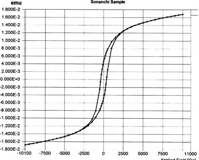
The magnetic analyses yielded hysteresis loop data both as a series of data points and as visual output. Two representative examples of the hysteresis loop behavior observed are shown in Figure 8 and Figure 9. Figure 8 shows the visual output from one of the samples from the Baixia Estate locality, while Figure 9 shows one from the Sonanchi Crater locality. The Baixia Estate sample shows what is likely either paramagnetic or antiferromagnetic behavior. In this case, it is more likely that the behavior is due to an antiferromagnetic response because none of the relevant Fe

emu

5000 7500 Applied

11000 Field [Oe]

---oxides that are likely creating the observed magnetic response exhibit paramagnetic behavior. The Sonanchi Crater sample shows a combination of linear and S-curve characteristics, suggesting that there are likely multiple forms of Fe oxides present in the sample. There is discussion later in this section of the likely Fe oxide form compositions of the analyzed samples.

emu Sonanchi Sample

1.800E-2 1.600E-2 - - - ~-1.400E-2 - - -- ---- --- ---1.200E-2 -1 1.OOOE-2 8.OOOE-3 6.OOOE-3 - _ _ _ _ _ _ _ _ _ _ _ _ _ _ _ _ _ _ _ 2.OOOE-3 - - - -O.OOOE+O --- - - - --2.000E-3 -4.000E-3 - --6.000E-3 --8.000E-3 -1.00E-2 -1.200E-2 ---- -- --1.400E-2 4--1.600E-2 --1.800E-2 --10100 -7500 -5000 -2500 0 2500 5000 7500 11000

Applied Field [0e]

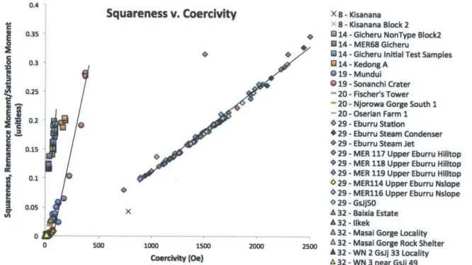
Characterization by Squareness and Coercivity

A combination of the main magnetic properties observed in this study provided

accurate characterization for three of the major obsidian sources surveyed, although the other analyzed sources were not easily distinguishable. Figure 10 shows the hysteretic squareness (Sq), which is a ratio of Mr and Ms, plotted against Hc for all analyzed samples. Several of the major obsidian sources tested (Groups 29, 14, and

19) show distinctive differences in both their average values for Sq and Hc, and also

the slope that the sample clusters create.

0.4

Squareness v. Coercivity X 8 - Kisanana

x 8 - Kisanana Block 2

0

0.35 _{0 14 - Gicheru NonType Block2}

N 14 - MER68 Gicheru

* * *14 -Gicheru Initial Test Samples

0.3 _{*14 - Kedong A}

@19 - Mundul 019 - Sonanchi Crater

0.25 _{-20 - Fischer's Tower}

20 - Njorowa Gorge South 1

-20 -Oserian Farm 1

3 0.2 _{29 - Eburru Station}

jj _{29 - Eburru} Steam _Condenser

+*29 -Eburru Steam Jet

0.15 _{* 29 -MER 117 Upper Eburru Hilltop}

* 29 -MER 118 Upper Eburru Hilltop

*29 -MER 119 Upper Eburru Hilltop

0.1 _{29 - MER114 Upper Eburru Nslope}

0 _{29 - MER116 Upper Eburru Nslope}

S* 29 - GsJJ5O

x _{A 32 - Baixia Estate}

A 32 -Ilkek

0 - A 32 - Masai Gorge Locality

00o 1000 1500 2000 2500 A 32 - Masai Gorge Rock Shelter

A 32 -WN 2 GsJJ 33 Locality

Coercy(Oe) _{L32 -WN 3 near GsjJ 49}

Saturation Moment/g Fe X 8- Kisanana

35 _{X 8 - Kisanana Block 2}

0 14 - Glcheru NonType Block2

0 14 - MER68 Gicheru

30~ 14 - Gicheru Initial Test Samples

S14 - Kedong A

* 19 -Mundul

25 @ 19 -Sonanchi Crater

-20 - Fischer's Tower

E 20 - Njorowa Gorge South 1

- 20 - 20 - Oserlan Farm 1

*29 - Eburru Station

*29 - Eburru Steam Condenser

cis * 29 - Eburru Steam Jet

* 29 -MER 117 Upper Eburru Hilltop

* 29 -MER 118 Upper Eburru Hilltop

10 _{* 29 - MER 119 Upper Eburru Hilltop}

0 29 - MER114 Upper Eburru Nslope

5 29 - MER116 Upper Eburru Nslope

0 29 - GsjJ5O

-. _{A 32 -Baixia Estate}

a-Fe203 $A 32 -ikek

0______- _.___ A 32 -Masai Gorge Locality

A 32 - Masal Gorge Rock Shelter A 32 - WN 2 GsJj 33 Locality

L 32 -WN 3 near GsJj 49

Figure 11. Plot of saturation moment (Ms) per gram of Fe in the sample, ordered by source group and locality. Weight percent Fe203 for all samples (except Masai Gorge, WN 2 and WN 3) found in Brown et al. 2013. Previously unpublished Fe203 values for these three (Appendix A: Table 1) were provided by Merrick (pers. com. 2014).

Saturation Moment and Fe Percentage Calculations

For the purposes of analysis, the magnetic responses of the samples were assumed to be completely caused by various forms of Fe in the samples, since Fe is the only magnetic mineral found in noticeable concentrations in the analyzed samples (Brown et al. 2013). The saturation moments obtained in this study and the Fe concentrations given for the samples in Brown et al.'s (2013) paper were used to determine the saturation moment per gram of Fe in each sample (see Figure 11). The calculated Ms/gFe values for the samples were then compared to literature values from pure samples of various Fe oxides to give an approximation of the forms

Approximate Percentage of Fe In a-Fe203 Form X8 -Kisanana

* * 0 8 - Kisanana Block 2

X .

*:.

0:- *14 -MER68 Gicheru

0.95 *14 -Gicheru Initial Test Samples

1 *14 - Kedong A

@19 - Mundul

@19 -Sonanchi Crater

- 20 - Fischer's Tower

- 20 - Njorowa Gorge South 1

C6 - 20 - Oserian Farm 1

0.85 _{* 29 -Eburru Station}

* 29 - Eburru Steam Condenser

* 29 -Eburru Steam Jet

0.8 *29 -MER 117 Upper Eburru Hilltop

@29 -MER 118 Upper Eburru Hilltop

0 29 -MER 119 Upper Eburru Hilltop

0.75 ₀ 29 -MER114 Upper Eburru Nslope

029 -MER116 Upper Eburru Nslope

* 29 - GsJj50

0.7 _{A 32 - Baixia Estate}

A 32 -Ilkek

A 32 - Masai Gorge Locality

0.65 _A 32 -Masal Gorge Rock Shelter

A 32 -WN 2 GsJj 33 Locality

Locality A 32 -WN 3 near Gsij 49

Figure 12. Plot of calculated approximate percentage of Fe in a-Fe203 form in the sample, ordered by source group and locality. Calculations were performed assuming only a-Fe203 and Fe304 forms existed in the obsidian.

of Fe present in the samples. Based on these calculations, the Fe in most of the analyzed sources was almost entirely in a-Fe203 form (see Figure 12). The only source that had a noticeably distinct percentage of a-Fe203 was Group 14, which had an average of about 20% less a-Fe203 than the rest of the sources tested.

Only the three most common iron oxides (a-Fe203, y-Fe203, and Fe304) were

included in the above analysis. For the purpose of analyzing the percentages shown in Figure 12, the percentages were calculated as if there were only a-Fe203 and y-Fe203 in the samples. This calculation was also performed assuming only a-y-Fe203 and Fe304, and there was 1% or less difference between the two calculated values for all the samples except for those in Group 14. These samples showed a maximum

difference of 4%, but the percentages of Fe oxides were still distinct enough to differentiate Group 14 from the other sources.

Precision Calculations

Machine precision for the VSM used in this study was analyzed by re-measuring the same sample several times. In addition, several samples from the same specimen

(same block of obsidian, but separately flaked off samples) were analyzed to assess the variance within a specimen. The results of these precision analyses are shown in Table 1.

Table 1. Precision calculations

Single Sample (machine precision analysis)

N = 4 Ms [emu/g] Mr [emu/g] Hc [Oe] Sq/Hc [/Oe]

Max 0.6102 0.1081 89.8478 0.0022 Min 0.5765 0.1035 83.6454 0.0020 (Max-Min)/2 0.0169 0.0023 3.1012 0.0001 Avg. 0.5896 0.1061 86.8748 0.0021 St. Dev. 0.0149 0.0020 3.0541 0.0001 % St. Dev 2.5206 1.9078 3.5156 4.0889

Separate samples from same specimen (testing variance within a single specimen)

N = 8 Ms [emu/g] Mr [emu/g] Hc [0e] Sq/Hc [/Oe]

Max 0.6696 0.1085 88.9444 0.0025 Min 0.5277 0.1020 71.5908 0.0020 (Max-Min)/2 0.0709 0.0032 8.6768 0.0002 Avg. 0.5975 0.1060 80.5700 0.0022 St. Dev. 0.0469 0.0026 5.5941 0.0001 % St. Dev 7.8552 2.4114 6.9431 6.1620

Discussion and Conclusions

Conclusions

Based on these magnetic analyses, it is possible to differentiate between three of the main obsidian source groups known to have been used archaeologically, source groups 14 (Kedong), 19 (Sonanchi), and 29 (Upper Eburru) using the classification from Merrick and Brown's work (Merrick and Brown 1984a). Each of the three groups has a distinctive slope when the hysteretic squareness is plotted against the coercivity of the samples. The differentiation between these three sources is

stronger than the differentiation seen in previous magnetic provenance studies in other regions (e.g. McDougall et al., 1983; Hillis et al., 2010; Vasquez et al., 2001; etc.), suggesting that such methods could have the potential to still be a useful metric for the characterization of Kenyan obsidians. The remaining three source groups sampled that could not be characterized all had very weak magnetic

responses, making it difficult to tell whether any pattern in the ratio of Sq to Hc was due to actual magnetic differences or background noise. This uncertainty could potentially be resolved by analyzing the temperature dependence of the properties measured here. The approximate percentage of Fe in various forms in the samples was also calculated. For almost all sources, the Fe in the samples was almost entirely a-Fe203. In the samples from source group 14, approximately 20-25% of the Fe is likely to be in either y-Fe20 3 or Fe304 forms. Both y-Fe20 3 and Fe30 4 have high Ms values, while c-Fe20 3 has a comparatively very small Ms value, so the percentage of a-Fe20 _{3was able to be determined to within 1% (or within 4% for the group 14}

samples), but how much of the remainder is y-Fe203 versus Fe304 is difficult to determine without further analysis.

Limitations

The samples analyzed here were not an ideal sample set for magnetic provenance analysis. They were not originally collected with magnetic studies in mind, but instead were gathered for a chemical analysis study (Merrick and Brown, 1984a; Brown et al., 2013), so most of the sampled localities only have one or maybe two samples each. Chemical analysis usually requires only a few specimens per source to obtain a useful characterization. Due to the chemical homogeneity of most obsidian flows, this approach is generally reasonable. However, since the magnetic

properties of obsidian are more varied across a flow -- and even within a single locality -- _{than chemical properties, it is necessary to collect many samples from}

each locality to acquire a complete picture of the magnetic properties of the obsidian (Frahm and Feinberg, 2013). If a more thorough magnetic provenance study were to be done in this region, more comprehensive sampling would likely be needed to fully characterize the sources.

Potential Future Work

There are several directions that future researchers could take this work. All of the tests in this study were performed at room temperature, which could be

supplemented with data on the temperature dependence of the samples' magnetic properties (as in Schmidbauer et al., 1986) to get a more in-depth understanding of the magnetic properties and material structure of the obsidian. In particular, the

temperature dependence of coercivity can be used to compare the average particle size of the iron oxide grains in the samples, which would provide comparative data about the cooling rates of the various obsidians in the region. These cooling rates could in turn be utilized as part of a more thorough characterization database for the region. In addition, temperature dependence tests would also give better information about the forms of Fe oxides present in the obsidians, which could provide an additional discriminant for characterization purposes.

Not only could this additional research help provide a more complete

characterization signature for inter-flow sourcing, this type of analysis also has more potential than any previous work that has been done in Kenya to provide locality-level characterization, as the Fe oxides present and the grain size of the mineral inclusions in obsidian are closely related to its cooling rate. Cooling rates varies across a given flow, possibly enough to make locality-level characterization possible. Such a study using the same samples that were available for this study could look at such intra-flow sourcing within only a handful of sources, as most of the sources with samples available for this study have specimens from only one or two different localities. Only recently was it acknowledged that the magnetic

variability within a flow might provide a useful tool for intra-flow obsidian sourcing rather than just being noise, but the first few studies that have looked into this possibility have shown promising initial results (Zanella et al. 2012; Frahm and Feinberg 2013).

Acknowledgements

Special thanks go to Professors Merrick and Beach, who were extremely patient with my questions about (respectively) the sample collection and how magnets work, to David Bono, who was of tremendous help with VSM wrangling, and to my parents for believing that I could get my degree done in four years. Further, I am immensely grateful to my late grandfather, Harold W. Krueger, for providing me with the funds to attend MIT. You are dearly missed.

Appendix A Magnetic ana Is data from all samples. Risanana, Block 1 36 No 8 0.034 36.064 1 7/12/13 0.0629 0.00753 2.50E-05 0.00332 25.474 0.11974 0.00040 0.101 0.04464 2.682 0.995 0.997 36 No 8 0.034 36.064 1.1 7/12/13 0.0629 0.00794 7.91E-06 0.00100 17.969 0.12623 0.00013 0.101 0.04464 2.828 0.994 0.996 36 No 8 0.034 36.064 2 7/12/13 0.0403 0.00520 2.23E-04 0.04280 778.16 0.12899 0.00552 0.101 0.04464 2.889 0.994 0.996 ^ 36 No 8 0.034 36.064 2.1 7/12/13 0.0403 0.00505 2.39E-05 0.00473 38.014 0.12538 0.00059 0.101 0.04464 2.809 0.994 0.996 36 No 8 0.034 36.064 3 7/12/13 0.0577 0.00707 1.24E-05 0.00175 15.690 0.12261 0.00022 0.101 0.04464 2.747 0.994 0.997 36 No 8 0.034 36.064 4 7/12/13 0.1286 0.01487 2.65E-05 0.00178 9.503 0.11565 0.00021 0.101 0.04464 2.591 0.995 0.997 36 No 8 0.034 36.064 5 7/12/13 0.0771 0.00979 1.55E-05 0.00158 10.394 0.12694 0.00020 0.101 0.04464 2.843 0.994 0.996 36 No 8 0.034 36.064 6 7/12/13 0.1444 0.01516 3.09E-05 0.00204 19.020 0.10497 0.00021 0.101 0.04464 2.351 0.996 0.997 36 No 8 0.034 36.064 7 7/12/13 0.0546 0.00663 1.50E-05 0.00226 21.118 0.12142 0.00027 0.101 0.04464 2.720 0.995 0.997 36 No 8 0.034 36.064 8 7/12/13 0.0502 0.00628 2.39E-05 0.00381 11.542 0.12506 0.00048 0.101 0.04464 2.801 0.994 0.996 36 No 8 0.034 36.064 9 7/12/13 0.0728 0.00875 1.29E-05 0.00147 12.243 0.12024 0.00018 0.101 0.04464 2.693 0.995 0.997 36 No 8 0.034 36.064 10 7/12/13 0.0890 0.01092 1.85E-05 0.00169 9.944 0.12266 0.00021 0.101 0.04464 2.748 0.994 0.997 Kisanana, Block 2 36 No 8 0.034 36.064 1 12/13/13 0.0330 0.00266 6.65E-06 0.0025 24.131 0.08061 0.00020 0.101 0.04464 1.806 0.997 0.998 36 No 8 0.034 36.064 2 12/13/13 0.0330 0.01505 7.53E-06 0.0005 4.844 0.45606 0.00023 0.101 0.04464 10.216 0.972 0.983 36 No 8 0.034 36.064 3 12/13/13 0.0493 0.00698 6.98E-06 0.0010 6.890 0.14149 0.00014 0.101 0.04464 3.169 0.993 0.996 36 No 8 0.034 36.064 4 12/13/13 0.0548 0.00990 4.95E-06 0.0005 5.173 0.18066 0.00009 0.101 0.04464 4.047 0.991 0.994 36 No 8 0.034 36.064 5 12/13/13 0.0519 0.00645 6.45E-06 0.0010 6.861 0.12428 0.00012 0.101 0.04464 2.784 0.994 0.996 Kedong A 1 No 14 -1.230 36.547 1 12/14/13 0.0630 0.03495 6.99E-03 0.2000 183.6 0.55476 0.11095 0.0336 0.01485 37.355 0.891 0.932 1 No 14 -1.230 36.547 2 12/14/13 0.0165 0.00905 1.77E-03 0.1955 153.3 0.54871 0.10727 0.0336 0.01485 36.947 0.892 0.933 1 No 14 -1.230 36.547 3 12/14/13 0.0529 0.02927 5.83E-03 0.1990 186.4 0.55333 0.11011 0.0336 0.01485 37.259 0.891 0.932 1 No 14 -1.230 36.547 4 12/14/13 0.0307 0.01864 3.49E-03 0.1870 163.4 0.60705 0.11352 0.0336 0.01485 40.875 0.880 0.925 1 No 14 -1.230 36.547 5 12/14/13 0.0341 0.01904 3.87E-03 0.2030 179.9 0.55834 0.11334 0.0336 0.01485 37.596 0.890 0.931 Glcheru (MER 63) 68 Yes 14 -1.185 36.549 1 6/5/13 0.0566 0.03428 4.00E-03 0.11654 35.19 0.60564 0.07058 0.0341 0.01507 40.183 0.882 0.926 68 Yes 14 -1.185 36.549 2 6/5/13 0.0629 0.04220 4.87E-03 0.11540 32.73 0.67089 0.07742 0.0341 0.01507 44.512 0.869 0.918 A One or more measured values for this sample were extreme outliers, likely caused by machine malfunction.

Appendix A (continued) 'I 68 Yes 14 -1.185 36.549 3 6/5/13 0.0600 68 Yes 14 -1.185 36.549 4 6/5/13 0.0300 68 Yes 14 -1.185 36.549 5 6/5/13 0.0501 68 Yes 14 -1.185 36.549 6 6/5/13 0.0481 68 Yes 14 -1.185 36.549 7 6/5/13 0.0813 68 Yes 14 -1.185 36.549 8 6/5/13 0.0422 68 Yes 14 -1.185 36.549 9 6/5/13 0.0514 68 Yes 14 -1.185 36.549 10 6/5/13 0.0453 Gicheru Non-Type, Block 1 68-69 No 14 -1.185 36.549 1.1 5/28/13 0.0434 68-69 No 14 -1.185 36.549 1.2 5/28/13 0.0434 68-69 No 14 -1.185 36.549 1.3 5/28/13 0.0434 68-69 No 14 -1.185 36.549 1.4 5/28/13 0.0434 68-69 No 14 -1.185 36.549 2 5/28/13 0.0391 68-69 No 14 -1.185 36.549 3 5/28/13 0.0213 68-69 No 14 -1.185 36.549 4 5/28/13 0.0306 68-69 No 14 -1.185 36.549 5 5/28/13 0.0307 68-69 No 14 -1.185 36.549 6 5/28/13 0.0371 68-69 No 14 -1.185 36.549 7 5/28/13 0.0153 68-69 No 14 -1.185 36.549 8 5/28/13 0.0225 68-69 No 14 -1.185 36.549 1 7/12/13 0.0434 Glcheru Non-Type, Block 2 68-69 No 14 -1.185 36.549 1 8/4/13 0.0101 68-69 No 14 -1.185 36.549 2 8/4/13 0.0178 68-69 No 14 -1.185 36.549 3 8/4/13 0.0203 68-69 No 14 -1.185 36.549 4 8/4/13 0.0370 68-69 No 14 -1.185 36.549 5 8/4/13 0.0329 68-69 No 14 -1.185 36.549 6 8/4/13 0.0354 68-69 No 14 -1.185 36.549 7 8/4/13 0.0463 68-69 No 14 -1.185 36.549 8 8/4/13 0.0295 68-69 No 14 -1.185 36.549 9 8/4/13 0.0430 0.03532 4.17E-03 0.11807 33.65 0.58865 0.06950 0.0341 0.01507 39.05 0.04047 4.70E-03 0.11602 31.52 1.34889 0.15650 0.0341 0.01507 89.49 0.03080 3.83E-03 0.12436 33.29 0.61471 0.07645 0.0341 0.01507 40.7& 0.02943 3.49E-03 0.11860 32.12 0.61178 0.07256 0.0341 0.01507 40.59 0.05463 6.70E-03 0.12263 33.49 0.67201 0.08241 0.0341 0.01507 44.58 0.02601 3.15E-03 0.12092 32.39 0.61633 0.07453 0.0341 0.01507 40.89 0.03104 3.81E-03 0.12273 32.87 0.60397 0.07412 0.0341 0.01507 40.07 0.02831 3.90E-03 0.13756 38.12 0.62504 0.08598 0.0341 0.01507 41.47 0.02648 0.02560 0.02502 0.02524 0.02465 0.01369 0.02049 0.01620 0.02073 0.00882 0.01334 0.02374 0.00582 0.01012 0.01230 0.01592 0.01953 0.01953 0.02565 0.01562 0.02511

4.69E-03 4.66E-03 4.49E-03 4.59E-03 4.22E-03 2.20E-03 3.32E-03 3.21E-03 4.02E-03 1.56E-03 2.43E-03 4.49E-03 8.95E-04 1.51E-03 1.82E-03 3.03E-03 2.89E-03 2.89E-03 3.86E-03 2.53E-03

0.17709 0.18181 0.17945 0.18188 0.17117 0.16046 0.16204 0.19824 0.19369 0.17696 0.18254 0.18888 0.15387 0.14875 0.14799 0.19024 0.14801 0.14801 0.15031 0.16229 89.09 89.85 84.92 83.65 84.13 71.59 76.62 79.92 88.94 76.04 83.67 93.49 75.20 72.95 76.13 75.71 69.11 69.11 70.97 70.09 0.61023 0.58995 0.57653 0.58149 0.63054 0.64267 0.66958 0.52770 0.55873 0.57654 0.59275 0.54712 0.57591 0.56860 0.60597 0.43017 0.59350 0.55159 0.55391 0.52938 0.10806 0.10726 0.10346 0.10576 0.10793 0.10312 0.10850 0.10461 0.10822 0.10203 0.10820 0.10334 0.08861 0.08458 0.08968 0.08184 0.08784 0.08164 0.06326 0.08592 3.53E-03 0.14058 66.68 0.58398 0.08209 0.0339 0.0339 0.0339 0.0339 0.0339 0.0339 0.0339 0.0339 0.0339 0.0339 0.0339 0.0341 0.0339 0.0339 0.0339 0.0339 0.0339 0.0339 0.0339 0.0339 0.01498 0.01498 0.01498 0.01498 0.01498 0.01498 0.01498 0.01498 0.01498 0.01498 0.01498 0.01507 0.01498 0.01498 0.01498 0.01498 0.01498 0.01498 0.01498 0.01498 40.726 39.373 38.477 38.808 42.081 42.891 44.687 35.218 37.289 38.477 39.559 36.300 38.435 37.948 40.442 28.709 39.609 36.812 36.967 35.330 6 0.886 0.929 5 0.735 0.834 4 0.881 0.925 0 0.881 0.926 6 0.869 0.918 2 0.880 0.925 2 0.883 0.927 0 0.879 0.924 0.881 0.885 0.888 0.887 0.877 0.874 0.869 0.897 0.891 0.888 0.884 0.894 0.888 0.889 0.882 0.917 0.884 0.893 0.892 0.897 0.925 0.928 0.930 0.929 0.923 0.921 0.918 0.936 0.932 0.930 0.928 0.934 0.930 0.931 0.926 0.948 0.928 0.933 0.932 0.936 0.0339 0.01498 38.974 0.886 0.929 0.02511