An adaptive Orthogonaly Division Multiplexing baseband modem for wideband wireless communication

An Adaptive Orthogonal Frequency Division

Multiplexing Baseband Modem for Wideband

Wireless Channels

by

Jit Ken Tan

B.S., Carnegie Mellon University (2003)

Submitted to the Department of Electrical Engineering and Computer

Science

in partial fulfillment of the requirements for the degree of

Master of Science

at the

MASSACHUSETTS INSTITUTE OF TECHNOLOGY

May 2006

©

Massachusetts Institute of Technology 2006. All rights reserved.

A uthor ...

...

Department of Electrical Engineering Ind Computer Science

May 12, 2006

C ertified by .

..

....

...

Charles G. Sodini

Professor

Thesis Supervisor

Accepted by ....

..

MASSACHUSETTS INSTITUTE OF TECHNOLOGY

NOV

0

2

2006

S. . . . . . . . . . . . . .

Arthur C. Smith

Chairman, Department Committee on Graduate Students

An Adaptive Orthogonal Frequency Division Multiplexing

Baseband Modem for Wideband Wireless Channels

by

Jit Ken Tan

Submitted to the Department of Electrical Engineering and Computer Science on May 12, 2006, in partial fulfillment of the

requirements for the degree of Master of Science

Abstract

This thesis shows the design of an Orthogonal Frequency Division Multiplexing base-band modem with Frequency Adaptive Modulation protocol for a widebase-band indoor wireless channel. The baseband modem is implemented on a Field Programmable Gate Array and uses 294,939 2-input NAND gates with a clock frequency of 128 MHz. The Frequency Adaptive Modulation algorithm is 6% of the entire baseband modem which means that it is of low complexity.

The baseband modem is then integrated with a RF Front End. The maximum transmit power of the RF Front End is 7.5 dBm. This prototype takes 128 MHz of bandwidth and divides it into 128 1-MHz bins. The carrier frequency is at 5.25 GHz. Measurements are taken with this prototype to investigate the concept of Frequency Adaptive Modulation. With a target uncoded Bit Error Rate of 10', it is found at distances of 1.0m to 10.8m, the data rate varies from 355 Mbps to 10 Mbps. The average data rate of this system is 2.57 times the average data rate without Frequency Adaptive Modulation. The fact that a Rayleigh channel is decomposed into Gaussian sub-channels through Frequency Adaptive Modulation is also verified.

Thesis Supervisor: Charles G. Sodini Title: Professor

Acknowledgments

I would like to thank the following: my advisor Charlie Sodini for his tutorage -I am fortunate to have an advisor who fosters both intellectual and professional develop-ment; Team members Farinaz Edalat, Nir Matalon, Khoa Nguyen and Albert Jerng who make the project I am working on possible; Undergraduate research assistants, Raymond Wu, Justin Pun and Indy Yu for their help in the project; Mark Spaeth for consultation on the practical aspects of putting a prototype together; Professor Sodini and Professor Lee's research group who enrich the intellectual environment in the office and making the office a fun place to work; Rhonda Maynard for her administrative help; My family who has emotionally and financially supported me undertaking my education here away from home; and God who has blessed me with this opportunity to be here.

This material is based upon work supported by the National Science Foundation under Grant No. ANI-0335256. Any opinions, findings, and conclusions or recommen-dations expressed in this material are those of the author(s) and do not necessarily reflect the views of the National Science Foundation.

Contents

1 Introduction

1.1 Wideband Transceivers ...

1.2 Use of OFDM in Wideband Transceivers . . . 1.3 Frequency Adaptive Modulation . . . . 1.4 MIT WiGLAN Node . . . . 1.5 Outline of Thesis . . . . 2 Wireless Gigabit Local Area Network

2.1 Indoor Channel Model . . . . 2.2 CP Requirement . . . . 2.2.1 Mathematical Form of OFDM with CP 2.2.2 CP Length . . . .

2.3 Frequency Diversity Order of WiGLAN . . . .

2.4 NFFT based on Frequency Diversity Order and

2.5 Key Parameters in the WiGLAN . . . . 2.6 Sum m ary . . . . 3 An 3.1 3.2 3.3 15 . . 15 . . 16 . . 17 . . 20 22 23 23 24 26 . . . . 28 . . . . 29 CP length . . . . 30 . . . . 31

OFDM Baseband Transceiver

Effect of RF Front End on sub-carrier usage . . . . . . . .

QAM ... ...

Practical Transmission Model . . . . 3.3.1 Effects of Carrier and Sampling Frequency Offsets . 3.3.2 Effects of Phase Noise . . . .

32 35 36 38 42 43 47

3.3.3 Bit Resolution of ADC and DAC . 3.4 Receiver Design . . . . 3.4.1 Packet Detection . . . . 3.4.2 CFO Estimation and Correction . . 3.4.3 Channel Estimation and Correction 3.4.4 Phase Tracking . . . . 3.5 OFDM Transmitter . . . . 3.5.1 Clipper . . . . 3.5.2 PA Control at the Transmitter . . . 3.6 Sum m ary . . . . 4 Frequency Adaptive Modulation

4.1 Networking Aspects on the WiGLAN . . . . 4.1.1 Integration of the Physical Layer with the MAC layer 4.1.2 Bit Error Rate . . . . 4.2 Step 1: SNR Estimation . . . . 4.2.1 SNR Estimation . . . . 4.2.2 Sub-carrier Modulation Assignment . . . . 4.3 Step 2: CSI Feedback . . . . 4.4 Step 3: D ata . . . . 4.5 Sum m ary . . . . 5 Results and Analysis

5.1 Logic Utilization of the WiGLAN Baseband Node . . . . 5.2 Measurement Test setup . . . . 5.3 Channel Measurements . . . . 5.4 A nalysis . . . . 5.4.1 Path Loss Exponent In the Lab . . . . 5.4.2 Decomposition of Rayleigh Channel to Gaussian sub-carriers . 5.4.3 Data Rate of the WiGLAN ignoring Frequency Adaptive

Mod-ulation Overhead . . . . . . . . 4 7 . . . . 48 . . . . 49 . . . . 5 1 . . . . 53 . . . . 55 . . . . 58 . . . . 6 1 . . . . 64 . . . . 65 67 68 68 68 69 71 74 76 78 79 81 81 87 88 89 97 98 100

5.4.4 Data Rate of WiGLAN with Frequency Adaptive Modulation

O verhead . . . . 102

5.4.5 Data Rate of a normal OFDM System . . . . 104

5.4.6 Comparison of WiGLAN to a normal OFDM system . . . . . 105

5.5 Sum m ary . . . . 107

6 Conclusions and Future Research 109 6.1 Conclusions . . . . 109

6.2 Future Research . . . .. 111

6.2.1 Adaptive CP . . . .. 111

6.2.2 Reduction of PAPR . . . . 112

6.2.3 Adaption of Pilot Sub-carriers . . . . 113

6.2.4 Development of Better SNR Estimation Scheme . . . . 113

6.2.5 Use of OOK . . . . 114

List of Figures

1-1 Spectral Efficiency Through Overlap and Orthogonality of the

sub-carriers . . . . 17

1-2 BER Performance for BPSK under Rayleigh and Gaussian Conditions 18 1-3 Frequency Adaptive Modulation Used: Optimization of Data Rate . . 19

1-4 Measurement: Frequency Adaptive Modulation In Action . . . . 19

1-5 RF Front End Schematic . . . . 21

1-6 W iGLAN Node . . . . 21

2-1 Need of a CP in a Wireless Channel . . . . 25

2-2 Simple Implementation of OFDM Baseband Modem . . . . 27

2-3 Example of the excess delay spread on a Power Delay Profile . . . . . 28

3-1 Entire OFDM Baseband Transceiver . . . . 35

3-2 Ease of Reconstruction Filter based on number of subcarriers used . . 37

3-3 Different in Constellations with same maximum power and same aver-age power ... ... 40

3-4 QAM Constellation Map . . . . 41

3-5 Complete baseband transmission model . . . . 43

3-6 Subcarrier symbol rotation due to SFO and CFO . . . . 44

3-7 ICI resulting from CFO 6f . . . . 45

3-8 OFDM symbol window drift due to sampling frequency offset . . . . . 46

3-9 Receiver Design . . . . 48

3-10 Double Sliding Window Packet Detection Algorithm . . . . 50

3-12 3-13 3-14 3-15 3-16 3-17 3-18 4-1 4-2 4-3 4-4 4-5 4-6

Protocol for Frequency Adaptive Modulation . . . . . Packet Structure during SNR Estimation . . . . SNR M argin . . . . Adaptive Modulation Assignment with target BER of Packet Structure during CSI Feedback . . . . Packet Structure during Data Transmission . . . . Baseband Modem Implementation on FPGA . . Location of transmitter-receiver pair in the Lab Measurements for Location A-B . . . . Measurements for Location C-D . . . . Measurements for Location D and E . . . . Measurements for Location F and G . . . . Measurements for Location H and I . . . . Measurements for Location J and K . . . . Mean SNR vs -10logio(d) . . . .

5-10 Rayleigh Fading Channel decomposed to Gaussian sub-carriers (Sys-tem BER> 2.4 x 10-6 and Sub-carrier BER> 2.2 x 10-4 shown) . . . 5-11 Data Rate vs Link Distance . . . . 5-12 Effective Data Rate vs. Link Distance . . . . Implementation of CFO Estimator and Corrector . . . . Implementation of Channel Estimator and Corrector . . . . Insertion of pilot subcarriers to estimate time-varying phase rotation Implementation of Phase Tracking Module . . . . OFDM Transmitter . . . . Rare Occurrence of Large Peaks in OFDM Signal . . . . Clipper Implementation . . . . .... ... 82 . . . . 86 . . . . 90 . . . . 9 1 . . . . 92 . . . . 93 . . . . 94 . . . . 95 . . . . 99 100 101 103 53 56 58 59 60 62 65 68 69 73 75 77 78 5-1 5-2 5-3 5-4 5-5 5-6 5-7 5-8 5-9

List of Tables

1.1 Summary of RF Front End Specifications . . . . 1.2 Summary of Baseband Specifications . . . . 2.1 Coherence Bandwidth in Indoor Conditions . . . . 2.2 Summary of Indoor Channel Characteristics for Link Distance up lo m . . . . 2.3 Summary of Key System Parameters based on the Channel . . . .

to

3.1 Modulation dependent variables . . . . 3.2 BPSK Encoding Table . . . . 3.3 4-QAM Encoding Table . . . . 3.4 16-QAM Encoding Table . . . . 3.5 64-QAM Encoding Table . . . . 3.6 256-QAM Encoding Table . . . . 4.1 SNRmargin (dB) for different N given x = 7-6

4.2 Making Modulation Assignment based on & .

5.1 Number of 2-input NAND gates of Transmitter and Receiver . . . . . 5.2 Number of 2-input NAND gates of IFFT/FFT Module . . . . 5.3 Estimated Number of 2-input NAND gates of Transceiver . . . . 5.4 Number of 2-input NAND gates of Frequency Adaptive Modulation

b locks . . . . 5.5 Link Distance for various measurements . . . . 5.6 Adaptive Modulation Assignment for Location A to D . . . .

22 22 30 32 32 . . . . 38 . . . . 38 . . . . 38 . . . . 39 . . . . 39 . . . . 39 . . . . 73 . . . . 76 83 83 83 84 85 89

5.7 Adaptive Modulation Assignment for Tx Location E to H . . . . 96 5.8 Adaptive Modulation Assignment for Tx Location I to L . . . . 96 5.9 _{Measured Mean SNR and System BER of a normal OFDM System in}

various locations (BER> 2.4 x 10-6 shown) . . . . 97 5.10 WiGLAN Data Rate for location A to L . . . . 101 5.11 Effective WiGLAN Data Rate And Data Loss from Overhead for

loca-tion A to K . . . . 104 5.12 Finding the highest QAM modulation that yield a BER < 10- for a

normal OFDM System at Locations A to L (BPSK BER > 2.4 x 10-6 shown)... ... 105 5.13 Data Rate for normal OFDM System at location A to K . . . . 106 5.14 Throughput gain of WiGLAN compared to Normal OFDM System . 107

6.1 Summary of Baseband Specifications . . . . 110 6.2 Summary of RF Front End Specifications . . . . 110

Chapter 1

Introduction

The Wireless Gigabit Local Area Network (WiGLAN) project [1] at MIT seeks to prototype a baseband modem that utilizes a combination of 1) Wide bandwidth 2)

Orthogonal Frequency Division Multiplexing (OFDM) and 3) Frequency adaptive modulation to drive data rate up in a wireless indoor environment. The focus of this thesis is to document the implementation of this prototype and the analysis of indoor

measurements using this prototype with a radio-frequency (RF) Front End.

1.1

Wideband Transceivers

The Shannon-Hartley Capacity Theorem states that the capacity C of the channel is the following function of the signal bandwidth W and the average signal-to-noise ratio (SNR)

C = W log2 (1 + SNR) (1.1)

Hence there is a natural tendency to increase the bandwidth W in today's pursuit of achieving higher data rate. Examples of this occurrence are manifested in the following wireless standards:

9 Local Area Networks: The most well-known wireless standard would be 802.11a [2] with a bandwidth of 20 MHz and an uncoded data rate of 72 Mbps. There is a new 802.11n proposal [3] to combine a bandwidth increase of 40 MHz together

with multiple antennas to drive the uncoded data rate up to 720 Mbps.

9 Personal Area Networks: There is an ultra-wideband proposal [4] to use 528 MHz bandwidth to achieve an uncoded data rate of 640 Mbps.

1.2

Use of OFDM in Wideband Transceivers

Increasing the signal bandwidth W for a data signal on a single carrier might be problematic if the frequency selective fading condition occurs

W >> We (1.2)

where W, is defined as the coherence bandwidth of the channel.

Definition 1.2.1. _{The coherence bandwidth, W, is a statistical measure of the range} of frequencies over which the channel can be considered flat (i.e. a channel which passes all spectral components with approximately equal gain and linear phase) [5].

If frequency selective fading occurs, a complex multi-tap equalizer is required. One method of mitigating frequency selective fading while maintaining a large bandwidth is OFDM. In OFDM, the entire channel bandwidth is divided into several narrow sub-bands where each sub-band will experience flat fading. The flat fading condition is favored in communication systems because it reduces the complex multi-tap equalizer in the frequency selective fading case to a simple one-tap equalizer.

In addition, OFDM is a spectral efficient modulation scheme as there is spectral overlap with the sub-carriers as seen in Figure 1-1. Recovery of data despite of spectral overlap is possible because each sub-channel is orthogonal to each other. Currently, the use of OFDM is quite pervasive in the today's wireless standards [2, 3, 4]

However the use of OFDM has its disadvantages:

1. The peak-to-average power ratio (PAPR) of the transmitted signal is very high. Distortion from non-linearity will result unless a power backoff of the power

0 E TONE: A B C D E____ .. ... \JJz "\"J/ Frequency

Figure 1-1: Spectral Efficiency Through Overlap and Orthogonality of the sub-carriers

amplifier (PA) is exercised. This leads to a situation where there is a tradeoff between power efficiency of the PA and non-linear distortion.

2. Due to the spectral overlap of the sub-channels, OFDM is sensitive to mis-matches in the transmit-receive oscillators, phase noise and Doppler effects. More details about OFDM systems will be provide in Chapter 3.

1.3

Frequency Adaptive Modulation

In today's wireless standards [2, 3, 4], there is a rate adaptation mechanism where the modulation scheme is changed subject to the constraint that this modulation scheme is the same for all OFDM carrier. This is optimal provided that all the sub-carriers are highly correlated (i.e. if one channel can support a particular modulation scheme, all the other sub-carriers would be able to support it too).

Let's examine the ramification of keeping the modulation scheme in each OFDM carrier constant when each carrier is independent. Independence of sub-carriers is typical in wideband communication where each sub-carrier is sufficiently spaced apart. In this scenario, it could make sense to estimate the SNR on each sub-carrier and adapt the modulation scheme on a sub-sub-carrier basis. This enables each sub-carrier to be fully utilized hence the throughput of the system should increase as a result of performing adaptive modulation on a per sub-carrier basis.

100 BER vs SNR for BPSK -Gaussian W 1-5-10 -0 5 10 15 SNR

Figure 1-2: BER Performance for BPSK under Rayleigh and Gaussian Conditions

Under the same scenario where each sub-carrier is independent, the attenuation on each sub-carrier can be modeled as Independently and Identically Distributed (iid) random variables drawn from a Rayleigh distribution. If all the sub-carriers use the same modulation scheme, it can be said that Rayleigh fading across the fre-quency dimension is experienced by the system. The defining characteristic of this Rayleigh fading is having data transmission even on sub-carriers experiencing deep fades. Frequency Adaptive Modulation can be used to counter this Rayleigh fading. The sub-carriers experiencing deep fades are not used. Essentially, the Frequency Adaptive Modulation has reduced the Rayleigh fading channel to independent Gaus-sian sub-channels. The Bit Error Rate (BER) performance of a Rayleigh Channel and a Gaussian channel for Binary Phase-Shift Keying (BPSK) is shown in Figure 1-2. Also note that channel coding performs better in a Gaussian channel compared to a Rayleigh channel [6]. When channel coding is applied to a system, greater gain is derived when Frequency Adaptive Modulation is used.

Having examined two extreme scenarios where all the sub-carriers are either cor-related or independent, it can be inferred that the goodness of Frequency Adaptive Modulation is related to the frequency diversity order of the system. The frequency diversity order can be defined as the number of independently fading propagation frequency paths. This can be expressed as a ratio of the signal bandwidth W to

10

10-2

cc-3 W10

10~-Adaptive Modulation Scheme

5 10 15 20

SNR 25 30 35

Figure 1-3: Frequency Adaptive Modulation Used: Optimization of Data Rate

30

20-co

41

SNR vs Freq 0256QAM 0640AM *160AM L4QAM *BPSK ENULL 0 Freq (MHz) 50

Figure 1-4: Measurement: Frequency Adaptive Modulation In Action coherence bandwidth of the channel.

w

Frequency Diversity Order =

We (1.3)

Chapter 5 will explore empirically the goodness of adaptive modulation under various indoor channel conditions. When performing Frequency Adaptive Modulation, the criterion of optimization can be one of the following:

1. Data Rate.

2. Average Transmitting Energy.

-BPSK +-4 GAM -16 QAM -64 QAM +-256 QAM

N

'-4 QAM

NULL BPSK 4 GAM 16 GAM 64 QAM 256 OAM

3. BER.

In this project, the goal is to optimize the data rate of the system while keeping the average transmitting energy constant and the BER of the system below a particular threshold. Specifically, the WiGLAN scheme adopted maximizes data rate by using the most efficient modulation in each sub-channel allowed by its SNR while maintain-ing a uncoded BER less than 10-. This is shown in Figure 1-3. In Figure 1-4, the scheme is applied to an actual channel and the resulting adaption is shown.

It should be noted that Frequency Adaptive Modulation requires significant chan-nel knowledge at the transmitter hence synchronization between the transmitter and receiver is required. The effective data rate can be expressed in the following equation

R * Tdata

Reff - ± TYt. (1.4)

Tdata + Tsyne

where

" Ref f is the effective data rate.

* R is the data rate during the payload.

" Tdata is the length of the payload.

" Toyc is the time needed for synchronization between transmitter and receiver. According to Equation 1.4, Ref f is optimized when Tdata is large. However, Tdata is limited by the expiration time to the channel knowledge acquired by the transmitter. In an indoor environment, the throughput gain of Frequency Adaptive Modulation is best appreciated as the channel is static for a relatively long time such as 10ms. Characteristics of the indoor channel will be explored in Chapter 2. In Chapter 5, the effective throughput gain is quantified with respect to Equation 1.4.

1.4

MIT WiGLAN Node

The WiGLAN Node is the prototype transceiver shown in Figure 1-6, used to conduct indoor channel experiments. The transceiver consists of two portions:

POWER AMPLIFIER

"FOUT

RFIN

Figure 1-5: RF Front End Schematic

Figure 1-6: WiGLAN Node

1. Baseband Modem: This is extensively documented in this thesis.

2. RF Front End: The RF Front End is a custom system made with discrete

components. The RF Front End Node Schematic can be found in Figure 1-5. More details can be found in [7]. A summary of this RF Front End specifications can be found in Table 1.1.

The summary of specifications for baseband modem can be found in Table 1.2. The baseband modem is implemented on a Xilinx SX35 Field Programmable Gate Array (FPGA) mounted on an Avnet Evaluation Board. System Generator for DSP

Parameter Value

Bandwidth 128 MHz

Carrier Frequency 5.25 GHz Maximum Output Power 7.5 dBm Noise Figure 4 dB Bit Resolution of DAC 10 bits Bit Resolution of ADC 8 bits Sampling Frequency 128 MHz

Table 1.1: Summary of RF Front End Specifications

Parameter Value

Sampling Frequency 128 MHz Sub-carrier Frequency Spacing 1 MHz Number of data sub-carriers 119 Number of pilot sub-carriers 8 IFFT/FFT Period 1 ps Cyclic Prefix (CP) .2 ps

Symbol Period 1.2 ps

Uncoded BER 10-1

Modulation Per Bin BPSK,

4,16,

64, 256

QAM

Max Link Distance 10 m

Table 1.2: Summary of Baseband Specifications

is the software tool utilized to generate the Register Transfer Level (RTL) code for the FPGA.

1.5

Outline of Thesis

Chapter 2 describes the indoor channel model and its effects on the system. Chapter 3 reviews the basic OFDM transceiver architecture and implementation. Chapter 4 delves into the adaptive modulation scheme. Chapter 5 documents the indoor channel measurements and analyzes it. Chapter 6 concludes and provides directions for further work.

Chapter

2

Wireless Gigabit Local Area

Network

In this chapter, the Wireless Gigabit Local Area Network (WiGLAN) specifications affected by the characteristics of the indoor environment are discussed, namely the Cyclic Prefix (CP), the system bandwidth and number of sub-carriers available for use.

2.1

Indoor Channel Model

In the wireless environment, the signal at the transmitter can travel on multiple paths to reach the receiver. The signal seen at the receiver will be the sum of the transmitted signal from multiple paths characterized with different amplitude and phase. In a wireless environment where motion is prevalent, the multiple paths taken by the transmitted signal to receiver will change over time.

Mathematically, the channel can be modeled as a Finite Impulse Response (FIR) filter with time-varying tap values.

h(T, t) = hi(t) .6(r - T) (2.1)

can be modeled as a linear and time-invariant (LTI) system

h(t) = - 6(t - ti) (2.2)

Definition 2.1.1. The coherence time, T, is a statistical measure of the time duration over which the channel impulse response is essentially invariant [5].

9

TC = 9 (2.3)

167rf M fm = v/A

where

" v is the maximum velocity of transceiver. " A is the wavelength of the carrier frequency.

In the context of the WiGLAN project with a carrier frequency of 5.25 GHz and the maximum velocity v of 1 m/s (walking speed) in an indoor environment,

T, as computed by Equation 2.3 is 24 ms. For the rest of the thesis, the channel

will be modeled as an LTI system as the assumption is made that continuous data transmission for the WiGLAN project will not exceed 10 ms.

2.2

CP Requirement

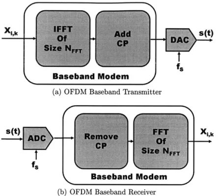
When transmitting in the wireless channel, the received Orthogonal Frequency Divi-sion Multiplexing (OFDM) signal can be modeled as shown in Figure 2-la. In this situation, Inter-symbol Interference (ISI) occurs between successive OFDM symbols as seen in Figure 1b. A CP can be inserted to avoid ISI as depicted in Figure 2-1c. Note that the length of the CP should be longer than the length of the channel impulse response for the condition of no ISI to hold true.

tx

s(t)

rx

r(t)

(a) Received signal model in a wireless channel

s(t)

h(t)

r(t) = s(t) * h(t)

(b) Channel Causes ISI without CP

s(t)

h(t) _{I t}

r(t) = s(t) * h(t) s*(t) 0 h(t)

0 = circular convolution I (c) Having CP prevents ISI

The next two sub-sections will express the mathematical form of an OFDM signal and find the length of the CP based on the length of the channel impulse response.

2.2.1

Mathematical Form of OFDM with CP

With the insertion of the CP, the mathematical form of the transmitted signal s(t)

looks like the following

s(t)

u(t)

+oo _K/2-1

1

S

Xik e 2,ksf(tc-iTsYM)u(t - iTSYM)

ITFT _{i=-00 k=-K12} 1 0;t<TFFT, 0 else. TFFT = NFFTfs Af = 1/TFFT TSYM TFFT +TCP where

" i is the time symbol index. " k is the frequency index.

" K is the number of sub-carrier used.

" Xi,k are the data symbols.

" Af is the sub-carrier spacing.

" TFFT is the IFFT/FFT period.

e NFFT is the maximum of sub-carriers.

*

f,

is the sampling frequency of the system.

* TCp is the length of the cyclic prefix.

(2.4)

(2.5) (2.6)

(2.7) (2.8)

f

(a) OFDM Baseband Transmitter

s(t) _X,

fs Baseband Modem

(b) OFDM Baseband Receiver

Figure 2-2: Simple Implementation of OFDM Baseband Modem

9 Tsym is the period of a OFDM symbol inclusive of the CP.

Based on Equation 2.4, the OFDM baseband transceiver can be implemented as shown in Figure 2-2.

In addition, the insertion of the CP converts linear channel convolution into circu-lar convolution. If si (t) is the transmitted ith OFDM symbol and ri (t) is the received

ith OFDM symbol, ri(t) has the following relationship

si(t) F- Si(f)

(2.9)

EFT

h(t) -+ H(f) (2.10)

ri(t) F+ Ri(f) = Si(f)H(f) (2.11)

The demodulated data symbol R,, can be expressed as a multiplication of the original data symbol Xi,k and a constant factor Hk. Hence to recover the data symbol,

Ih(t)12 (dB) 0

t

t

+

_O

Excess Excess Delay (ns) Delay Spread (X dB)

Figure 2-3: Example of the excess delay spread on a Power Delay Profile a simple one-tap equalizer is required.

Ri,k = Ri

)

(2.12) TFFT k Xi,k = Si( ) (2.13) TFFT k Hk = H( T ) (2.14) Ri,k = Xi,kHk (2.15)

2.2.2

CP Length

The length of CP needs to be longer than the length of the channel response. The length of the channel response can be quantified using excess delay spread (X dB) of the channel.

Definition 2.2.1. The excess delay spread is defined to be the time delay during which multipath energy falls to X dB below the maximum

[5].

An example of the excess spread can be found in Figure 2-3

The value of X should be based on the noise floor faced by the receiver. Multipath components below the noise floor do not contribute significantly to ISI and therefore

can be discounted. A conservative way of choosing X is to determine the maximum noise floor the system can tolerate with its most efficient modulation scheme without compromising the Bit Error Rate (BER). In the context of the WiGLAN, the most efficient modulation scheme is 256 Quadrature Amplitude Modulation (QAM) with a target BER of 10-. The minimum signal-to-noise ratio (SNR) required for this is 28.42 dB which corresponds to X = 28.42 dB [8].

Another fact to note is that as the link distance increases, the excess delay spread (X dB) increases. Physically, it means that the difference between shortest path and the longest path from the transmitter and receiver increases as a function of link distance. In the WiGLAN system, the maximum link distance is 10m. As reported in [8], for a link distance up to 10m, X = 30 dB and a center frequency of 5 GHz, the excess delay spread is bounded by 70 ns.

However, in a practical OFDM system, having the length of CP be exactly the excess delay spread (30 dB) leaves no room for timing estimation errors. Hence, in the conservative design of the WiGLAN system, the length of CP used is 200 ns. It's noted that the data rate of the system decreases as the length of CP increases. The exact relationship of the effective data rate Rett can be expressed as the following

Ref f = TFFT -Bits Per OFDM Symbol (216)

TCP + TFFT

2.3

Frequency Diversity Order of WiGLAN

Recall from Section 1.3, the goodness of Frequency Adaptive Modulation of the WiGLAN system is dependent on the frequency diversity order of the system which can be expressed as the ratio of the signal bandwidth W to the coherence bandwidth

Wc. In the literature, the W, is normally not explicitly stated. However, W, can be

Link Distance oU,[8] We/2wr(Equation 2.17)

1m 2ns 10MHz

10 M 10 ns 2 MHz

Table 2.1: Coherence Bandwidth in Indoor Conditions The equations for W, [5] and ur [8] are as follows

We ~ 7 (2.17)

50a,

U' = (Ti -Tm)2|h(i)12 (2.18)

am= ET - h(i)12 (2.19)

The coherence bandwidth in indoor conditions is summarized in Table 2.1.

For any given We, to obtain the maximum frequency diversity order, the signal bandwidth would be as large as possible. The signal bandwidth W in an OFDM system is bounded by the sampling frequency

f,.

With today's technology of proto-typing the baseband modem on Field Programmable Gate Array (FPGA), it is found that the fastest sampling frequency without having to resort to intensive pipelining of the system is 128 MHz.

For the WiGLAN system where f, = 128 MHz and W, in Table 2.1, the frequency diversity order (= W/Wc) can range from 12.8 to 64. For Frequency Adaptive

Modu-lation to show an improvement compared to today's wireless standards [2, 3, 4] where the same modulation for all sub-carriers is used, frequency diversity order needs to be greater than 2 (i.e. at least two independent fading frequency paths).

2.4

NFFT

based on Frequency Diversity Order and

CP length

The NFFT selected for the WiGLAN is 128. There are several design considerations to arrive at this final number:

1. To enable a simple implementation of the Inverse Fast Fourier Transform (IFFT) and fast fourier transform (FFT), NFFT should be a power of 2 [9].

2. To fully utilize the frequency diversity order in the WiGLAN system, the num-ber of sub-carriers should be at least the maximum frequency diversity order available to the system (i.e. NFFT - 64). Increasing NFFT further will not

yield better frequency diversity order.

3. For faster data rate, the TCp/TFFT should be kept as low as possible where

TFFT NFFT (i.e. keeping the ratio of overhead to payload small). A good rule

of the thumb from wireless standards [2, 3, 4] is the following:

TCp/TFFT < 0.3 (2.20)

From Section 2.2.2 and 2.3, it is determined that Tc = .2 ns and f, = 128 MHz. Under these conditions, it is found from equation 2.20 that NFFT > 85.3.

2.5

Key Parameters in the WiGLAN

From previous sections, several key parameters of the WiGLAN has been computed: " From Section 2.2.2, Tcp = .2 ns for a maximum link distance of 10m.

" From Section 2.3,

f,

= 128 MHz. " From Section 2.4, NFFT = 128.

From the above information and Equations 2.6 to 2.8, the other key parameters of the system can also be derived

* TFFT 1

Ys-* TSYM = 1.2 mus.

Specification Value Coherence Time 24 ms Excess Delay Spread(30 dB) 70 ns

Coherence Bandwidth 2 to 10 MHz

Table 2.2: Summary of Indoor Channel Characteristics for Link Distance up to 10m

Variable Value

FFT Size, NFFT 128

CP Length, TCP, -2ps IFFT/FFT Period, TFFT 1 Mus OFDM Symbol Period, TSYM 1.2 /-s Inter sub-carrier spacing, Af 1 MHz

Maximum transmission Time 10 ms Maximum Link Distance lOm Frequency Diversity Order 12.8 to 64

Table 2.3: Summary of Key System Parameters based on the Channel

2.6

Summary

Table 2.2 summarizes the indoor channel characteristics for link distance up to 10m. Table 2.3 summarizes the key system parameters based on the channel. Several key points are made in this chapter:

" Continuous data transmission is confined to at most 10 ms so that the channel can be treated as an LTI system. An algorithm catering to a time-varying channel can be difficult to implement.

" A conservative CP of 200ns is inserted per OFDM symbol to prevent ISI. * The WiGLAN system has a frequency diversity order of 12.8 to 64 which

indi-cates that frequency adaptive modulation is ideal for this system. " NFFT is selected to be 128.

- It is big enough to exploit the frequency diversity order available in the channel.

- It is small enough so that the resultant degradation to data rate due to insertion of CP is kept minimal.

Chapter 3

An OFDM Baseband Transceiver

From Chapter 2, a simple Orthogonal Frequency Division Multiplexing (OFDM) transceiver in the presence of a wireless channel is presented. However, the OFDM transceiver is more complex due to non-idealities from the radio-frequency (RF) Front End. In this Chapter, the entire OFDM baseband transceiver chain with the trans-mission model as seen in Figure 3-1 will be explored.

Bits transmitted are first Quadrature Amplitude Modulation (QAM)-modulated to symbols Xi,k. _{Each symbol is designated to frequency bin of index k and an}

OFDM symbol of time index i. Conversion of Xi,k from the frequency domain to the time domain is performed by the OFDM transmitter. The time domain signal is sent through the transmission model. The transmission model models the wireless channel as well as the RF Front End non-idealities. The signal from the output of the transmission model is then processed by the OFDM receiver. The receiver will compensate for the effects of the transmission model. The output of the receiver

is

Zi,k

which is the estimate of the QAM-modulated symbol Xi,k sent. The QAM demodulator will then convert Xi,k _{to bits. Note that in the entire OFDM transceiver,}

not all the frequency bins are capable of being used due to the design and non-idealities of the RF Front End.

In the next few sections, the effect of the RF Front End on sub-carrier usage as well as the elements of the OFDM transceiver chain such as the QAM blocks, the transmission model, the OFDM receiver and transmitter will be explored in more details.

3.1

Effect of RF Front End on sub-carrier usage

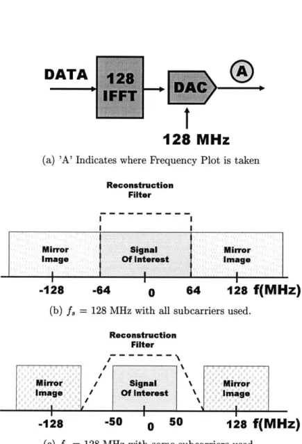
In a practical implementation, not all the sub-carriers are used. As shown in Figure 3-2b, when all the sub-carriers are used, the bandwidth of the signal will be

f,

and the signal and the mirror images will be next to each other. Hence, a brickwall reconstruc-tion filter is required to filter out the mirror images. Brickwall reconstrucreconstruc-tion filters are impossible to construct as there is no transition region from the passband fre-quencies to the stopband frefre-quencies. The constraints on reconstruction filter can be more relaxed by increasing the separation between the signal and the mirror images. This can be accomplished by not using some sub-carriers at the higher frequencies which is depicted in Figure 3-2c.

In addition, the DC sub-carrier is not used. There are intrinsic DC offsets occur-ring in the RF Front End which are removed by DC-coupling capacitors to achieve optimal swing in RF components. As a result, if a signal is sent at the DC sub-carrier, DC-coupling capacitors will either remove or highly attenuate that signal.

As later discussed in Section 4.3, during the stage of WiGLAN transmission when Channel State Information (CSI) per sub-carrier is unknown,

* DC sub-carrier is never used.

* 27 sub-carriers with the highest frequency components are not used to send when synchronization information is sent from the receiver and the transmitter because these sub-carriers lead into the transition band of the reconstruction. These sub-carriers might be heavily attenuated leading to high errors if data is

DATA

128 MHz

(a) 'A' Indicates where Frequency Plot is taken

Reconstruction Filter

Mirror Signal Mirror

image Of Interest Image

I

I

I

-128 -64 0 64 128

f(MHz)

(b) f, = 128 MHz with all subcarriers used.

Reconstruction Filter

Mirror / Signal Mirror

Image / Of Interest \ Image

1

I

'

I

-128 -50 0 50 128

f(MHz)

(c)

f,

= 128 MHz with some subcarriers used.

Modulation Nbit, Kmod BPSK 1 1 4-QAM 2 1/f2 16-QAM 4 1 V5 64-QAM 6 1/

v4

256-QAM 8 1/ 170

Modulation dependent variables

Input bit(bo) I

Q

0 -1 0

1 1 0

Table 3.2: BPSK Encoding Table

sent on them.

It is possible that the signal-to-noise ratio (SNR) of those sub-carriers is high enough to carry some data. Once CSI is available to the transmitter and re-ceiver, the frequency adaptive modulation algorithm can assign data to those sub-carriers that are data-capable despite being in the transition band of the reconstruction filter.

3.2

QAM

At the transmitter, each kth sub-carrier can either not be used or be modulated using Binary Phase-Shift Keying (BPSK), 4-QAM, 16-QAM, 64-QAM or 256-QAM. Depending on the modulation scheme, each modulated symbol can represent Nbit, of data bits as shown in Table 3.1. The bits are first converted to I/Q pairs according to the encoding tables shown in Table 3.2 to Table 3.6 with the input bit, bo, being

Input bit(bo) I Input bit(b1)

Q

0 -1 0 -1

1 1 1 1

Table 3.3: 4-QAM Encoding Table Table 3.1:

Input bit(bobi) I 00 -3 01 -1 11 1 10 3 Input bit(b2b3)

Q

00 01 11 -3 -1 1

10

j3

Table 3.4: 16-QAM Encoding Table

Input bit(bob1b2) I 000 -7 001 -5 011 -3 010 -1 110 1 111 3 101 5 100 7 Input bit(bb4b)

Q

000 -7 001 -5 011 -3 010 -1 110 1 111 3 101 5 100 7

Table 3.5: 64-QAM Encoding Table

Input bit(bob1b2b) I 0000 -15 0001 -13 0011 -11 0010 -9 0110 -7 0111 -5 0101 -3 0100 -1 1100 1 1101 3 1111 5 1110 7 1010 9 1011 11 1001 13 1000 15 Input bit(b4bb 6b7)

Q

0000 -15 0001 -13 0011 -11 0010 -9 0110 -7 0111 -5 0101 -3 0100 -1 1100 1 1101 3 1111 5 1110 7 1010 9 1011 11 1001 13 1000 15

Same Max Power 10 1 6-QOAM 2 X4-QAM * 0 0 * o 0 0 0 S0 o o 0 0 -1 * 0 0 40 -2 -2 -1 0 1 2 0

Same Average Power

0 16-QOAM 2 X4-QAM o 0 0 0 p ₀ X 0 0 0 o 0 0 0 1 x x o 0 0 0 2[ -2 -1 0 1 2

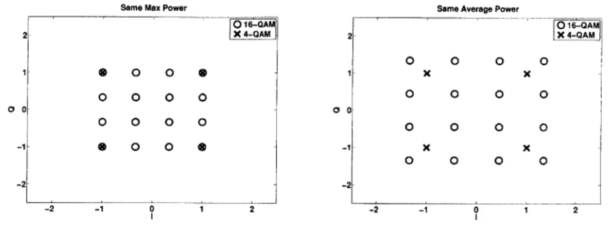
(a) Constellations with same maximum power (b) Constellations with same average power Figure 3-3: Different in Constellations with same maximum power and same average power

the earliest in the stream. With the I/Q pairs, the output of the QAM Modulator,

X is given by

X = (I +jQ) X KMOD (3-1)

where KMOD is given by Table 3.1. The purpose of KMOD is to achieve the same average power for all mappings (i.e. an average power of 1). An example of constella-tions with the same maximum power and same average power is shown in Figure 3-3. The QAM modulator is implemented as a symbol lookup table based on the input bits.

Note that the bits are gray-coded (i.e. adjacent values of I or

Q

only differ by a bit). The symbol error that is most common is when a sent symbol gets demodulated as an adjacent symbol. Gray coding limit the bit error of such an occurrence to 1 bit per symbol.

At the receiver, the input to the QAM demodulator is X, an estimate of the sent X provided by the OFDM receiver. Assuming that getting a bit 0 or 1 is equiprobable, the optimal detection algorithm is to decode the bits of sent symbol that is nearest to the received X. In Figure 3-4, each sent symbol X is visually associated with a square area that X must lie in for X to get decoded as X. The QAM demodulator is been implemented as a series of boundary comparisons to isolate the square area that

BPSK

0

0-I

(a) BPSK Constellation Map

16-QAM

4

2-a 0

-2

(c) 16-QAM Constellation Map

1f 14 12 ic a a -2 -4 -2 -4 -10 -12 -14 C 0 21 a -6 -4 -2 0 2 4 6 6

(d) 64-QAM Constellation Map

256-AM

Figure 3-4: QAM Constellation Map -16-14-12-10 -8 -6 -4 -2 0 2 4 6 8 10 12 14 16

(e) 256-QAM Constellation Map

4-QAM

2

- ~ 0 2

(b) 4-QAM Constellation Map

64-AM C

4

2

X lies in. Upon locating the square area, the associated decoded bits are produced

at the output of the QAM demodulator block.

3.3

Practical Transmission Model

A practical transmission system can be modeled as shown in Figure 3-5 [10]. The parameters shown in Figure 3-5 in relation to RF Front End are the following:

1. The sampling frequency of the Digital-to-Analog Converter (DAC) at the trans-mitter

f,

and the sampling frequency of the Analog-to-Digital Converter (ADC) at the receiver f' are different. The Sampling Frequency Offset (SFO) ( is de-fined as follows: TI - T (3.2) 1 TS _fS 1 Ts''

2. At the transmitter, there is an oscillator which modulates the baseband signal to passband. Similarly, at the receiver, there is an oscillator which demodulates the passband signal to baseband.

(a)

6f

is the Carrier Frequency Offset (CFO) between the transmitter and the receiver oscillator.

(b) 6(t) represents the phase noise in the oscillators. The frequency generated by practical oscillators varies over time. This variation can be modeled as noise in the phase of the received signal.

3. n(t) is the Additive White Gaussian Noise seen by the receiver. The thermal noise faced by the RF front end as well as the quantization noise of the data converters contributes to n(t).

Simple OFDM TX Simple OFDM RX mamanimail k Transmission Model

T

_n(t) 1'

Figure 3-5: Complete baseband transmission model

The subsequent subsections will discuss the effects of the transmission model on the OFDM system.

3.3.1

Effects of Carrier and Sampling Frequency Offsets

Recall from Section 2.2.1, that in the presence of the channel h(t), R,k = HkX i,k

(Equation 2.15). Ri,k with respect to Figure 3-5 (in the absence of 6(t)) can be expressed as [10]

Ri,k =(e jrk . e j2rk (iNsYM +NCP)/NFFT) .si(7rqk)HkXi,k

+ ICI + ni,k

where

* ICI is defined as the Inter-carrier Intererence.

(3.3)

* ni,k is the complex-valued Additive White Gaussian Noise (AWGN) resulting from n(t) with variance o.

69 2 rC(Nsy,/NFFT) A2 , 2 )r6 frSy. _ _ _ _ _ _ _

k

Figure 3-6: Subcarrier symbol rotation due to SFO and CFO

* NCP = [Tcp/Ts]

* NSYM = NCP + NFFT

0 si(X) = _sin(x/NFFT)sin(x)

* 4 6_{fTFFT + (k}

There are three effects from CFO and SFO in the system as indicated in Equa-tion 3.3:

1. Time-variant Symbol Rotation: ei2,0k(iNSYM+NCP)/NFFT is the time-variant

com-ponent in the equation. Going from one OFDM symbol to the next in time will yield a phase increment of 4Pk.

4k = 27rkNSYM/NFFT _(3.4)

There is a linear relationship between 6_{Ok and k as shown in Figure 3-6.}

2. SNR Degradation:

e ICI

from

CFO: As shown in Figure 3-7, CFO causes sampling of data to be off from the ideal points. This results in the reduction of the desired signal's amplitude and introduces interference from other carriers. The

E (a) E A B C D E

/

V4

/

/

\

Bf Frequency

Sampling of data in the frequency domain off by 3f

A B C D E

(b) Non-ideal sampling of data in frequency domain causes ICI Figure 3-7: ICI resulting from CFO 6f

OFDM symbol window For C 0 I INsym (I+1)Nsym n symbol windov -1 Nsym Receiver window -4

Figure 3-8: OFDM symbol window drift due to sampling frequency offset

degradation DCFO in dB to the current SNR caused by CFO

6f

can be expressed as the following[11]

10

DCFOlO(~fTFFT

sNR (3.5) From equation 3.5, it can be seen that as the SNR requirement is higher, the sensitivity to CFO increases. In the context of the WiGLAN, the highest SNR requirement occurs when 256-QAM is used (28.6 dB for BER = 10-3 ). With DCFO set to a negligible loss of 0.5 dB, the maximum CFO tolerated by the WiGLAN system is 6 kHz.

ICI from SFO: The SNR degradation DSFO;k from SFO on the kh sub-carrier with SNRk is given by [12]

DSFO;k = 1010910(1 + 1SNRk- (k( f fs)) ₂) (3.6)

From Equation 3.6, the degradation increases when k increases or SNRk increases. To obtain the maximum degradation DSFO;k, the highest SNR requirement of 28.6 dB for the use of 256-QAM and k of -64 are considered. Hence for the WiGLAN with

fs

of 128 MHz and the sampling clocks of 100 parts per million (PPM), the maximum degradation Dk from Equation 3.6

is 1.4 dB. This degradation is relatively negligible.

3. Frame Drifting from SFO - Assuming the start of the 0th OFDM symbol is

perfectly aligned, the drift of ith OFDM symbol is -i(NsyM as shown in Figure 3-8. The sampling clocks are specified at 100 PPM. Hence the maximum drift that can occur is 1 sample for every 5000 samples.

3.3.2

Effects of Phase Noise

Phase noise causes Inter-carrier Intererence (ICI). The degradation DPN in dB to the current SNR caused by phase noise can be expressed as the following[11]

10 11

DPN - 10 -= 1 (4wTFFT/3) -SNR (3.7)

10 60

where is the oscillator linewidth. Besides ICI, phase noise causes each sub-carrier in an OFDM symbol to be rotated by Common Phase Error (CPE) [13]. CPE only varies from one OFDM symbol to the next. If the CPE is slowly varying over time, it can be estimated and corrected for.

3.3.3

Bit Resolution of ADC and DAC

The ADC quantizes the signal and sends it to the digital baseband for processing. The act of quantization introduces noise to the system. Considering the quantization noise and the signal's PAPR, the SNR of a B bit ADC can be calculated as follows [14]

SNR(dB) = 6.02(B - 1) + 10.8 - PAPR(dB) (3.8) where the PAPR(dB) is the peak-to-average power ratio of the signal.

As it is later discussed in Section 3.5.1, the PAPR of the signal is at 16 dB. The ADC used in the WiGLAN is 8 bits. Using Equation 3.8, the SNR due to quantization noise is calculated to be 36.9 dB. This SNR also serves as an upper bound for the achievable SNR in an actual system where there are more noise sources.

r[n]

Q-ADC

-Figure 3-9: Receiver Design

Empirically, it is found that using a 10-bit DAC over 8-bit DAC yields approxi-mately 3 dB worth of SNR improvement. In general, DAC of higher bit resolution are easier to find than ADC with equivalent bit resolution. For the conservative design of the WiGLAN, a 10-bit DAC and a 8-bit ADC is used.

3.4

Receiver Design

In consideration of the transmission model from Section 3.3, the receiver design is presented in Figure 3-9. To recover the sub-carrier data to be passed into the QAM demodulator, the received signal r[n] is passed through the following sequence of blocks:

" Packet Detection: This module is responsible for detecting the start of the packet.

" CFO Estimator/Corrector: Once the packet is detected, the CFO is estimated and corrected to minimized the effects of ICI in the later stages.

" CP Removal: The Cyclic Prefix (CP) that is inserted to guard against Inter-symbol Interference (ISI) is removed prior to the FFT.

" FFT: Perform a transform on each OFDM symbol in time to obtain the

sub-carrier symbols.

" Channel Estimator/Corrector: Estimate and correct the channel-induced at-tenuation and phase rotation on the sub-carrier symbols.

" Phase Tracking: Estimate and correct for time variant phase rotation on the sub-carrier symbols caused by CFO, SFO and phase noise.

" SFO Estimator/Corrector: Estimate the SFO by processing side-products of phase tracking. This module will correct for the OFDM Symbol Window Drift by indicating to the CP Removal Module to advance or delay by a sample when appropriate. This module also indicates to the channel corrector module to compensate the phase changes in the Frequency domain from the advance or delay of a sample.

3.4.1

Packet Detection

The algorithm employed is the double sliding window packet detection shown in Figure 3-10 [15]. The variables A, and B, are obtained from the received signal r[n] by NFFT-l An= r[n - i]12 _(3.9) i=O NFFT Bn= Ir[n + i]12 _(3.10)

The peak E[Mn] occurs when index n is exactly the start of the packet (i.e. An would consist of signal and noise and Bn would consist purely of noise).

E[M] peak = SNR + 1 (3.11)

Peak

Mn=A,/8n

... / . . ... ... Threshold

Figure 3-10: Double Sliding Window Packet Detection Algorithm

In a practical implementation, the peak finder is limited to a particular window size. The peak finder commences the search for the peak when M passes a certain threshold. From Equation 3.11, this threshold should be set to SNRin + 1 where

SNRmin is the minimum SNR the system is expected to support. The SNRin =

7 dB in the context of the WiGLAN system. This comes from the fact that the minimum required SNR for least efficient modulation BPSK to meet the targeted BER is 7 dB. From Figure 3-10, it is observed that the peak occurs at most NFFT

samples (the window size of A) after the threshold is detected. Hence the peak finder has a window size of

NFFT-The WiGLAN implementation of the packet detection is shown in Figure 3-11. Essentially, the packet detection algorithm senses for a large power increase to search for a packet. A DC offset in the system will diminish this power jump decreasing the efficiency of this packet detection algorithm. Hence inherent DC offset in the RF Front End necessitates the need of a DC Bias Removal filter.

The DC Bias Removal Filter used has a structure shown in Figure 3-11c[16]. The a factor is set to 0.5 as a multiplication by a power of two involves only bit shifting which is simpler than having to use an actual multiplier with built-in latency. Though ideally, the higher alpha factor will be better as seen from comparing Figure 3-1Id and Figure 3-11e. All alpha factors will remove the DC component completely. However, a higher alpha factor will attenuate lower frequency bins less and the amplification

on the higher frequency bins are closer to unity gain.

3.4.2

CFO Estimation and Correction

If there are two identical symbols each of NFFT samples, the Maximum Likelihood (ML) CFO estimate 6f can be represented as a function of the cross-correlation z between these two symbols[15]

-27r6 fT, = FT (3.12) NFFT-l z = ( r*[n]r[n - NFFT n=O NFFT-1 E

S

r[n]|]2e-j2,r6fT8NFFT n=O

At high SNR, the performance of this algorithm can be quantified by the following[17]

Var(-27rS'fT) = Var( ZZ) NFFT (NFFT)2 NFFT SNR 1 ₁ (3.13) (NFFT )3 SNR

One limitation in this algorithm is that 27r6fTSNFFT must lies between [-7r, 7r].

Hence the acquisition range of 6f is as follows 1

6f < (3.14)

2_TsNFFT

In the context of the WiGLAN, the maximum tolerable CFO is 500kHz. The max-imum error on the carrier oscillator is at 50 PPM. In the 802.11a standard [2], the carrier oscillator is specified at 20 PPM. Hence, the maximum CFO arising from the 802.11a oscillators are 209.6kHz which is easily corrected by the CFO algorithm. Due to cost issues, the cheaper WiGLAN oscillators used is at 50 PPM, giving a maximum possible CFO of 524 kHz. To circumvent a large uncorrectable CFO, the prototypes

BN AN .,nahl. Start Of Packet --- + 1 B,-' A,

(a) Block Diagram Implementation of Packet Detection

ILAN :i~m

WL

-T

I/N

Ij

I1

a

(b) N-point Moving Average Filter 5 1 -5 -10- -15- -20--60 -40 -20 0 20 k (Frequency Index) 40 60

T1

(c) DC Bias Removal Filter

.10 - .15-.20 -60 -40 -20 0 20 k (Frequency Index) 40 60

(d) Frequency Response of DC Bias Removal Re-(e) Frequency Response of DC Bias

moval Filter a = 0.5 moval Filter a = 0.8

Removal

Re-Figure 3-11: WiGLAN Implementation of Packet Detection

'(Ntj BN AN xfW " y.nf

N

F

-1 Ja bt II -- I -- O~ KAl An] 4"1] I ra-V