Adaptive Mesh Euler Equation Computations of Vortex Breakdown in Delta Wing Flow

(1)

Adaptive Mesh Euler Equation Computation of

Vortex Breakdown in Delta Wing Flow

by

David Laurence Modiano

S. B. Massachusetts Institute of Technology (1987) S. M. Massachusetts Institute of Technology (1989)

SUBMITTED TO THE DEPARTMENT OF

AERONAUTICS AND ASTRONAUTICS

IN PARTIAL FULFILLMENT OF THE REQUIREMENTS FOR THE DEGREE OF

Doctor of Philosophy at the

Massachusetts Institute of Technology

February 1993

@Massachusetts

Institute of Technology 1993

Signature of Author

Certified by

Thesis Supervisor Head, / 44

Certified by

Accepted by

/

Department of Aeronautics and Astronautics February, 1993 Professor Earll M. Murman Department of Aeronautics and Astronautics

Professor Mirten Landahl Department of Aeronautics and Astronautics

Dr Michael B. Giles

o-4ft oyce Reader in CFD, Oxford University

N ... .- - Professor Harold Y. Wachman

Chairman, Department Graduate Committee MASSACHUSETTS INSTITUTE

OF TFCHjn ny

FEB 17

1993

UB RARIES

(2)

.,-Adaptive Mesh Euler Equation Computation of Vortex

Breakdown in Delta Wing Flow

by

David Laurence Modiano

Submitted to the Department of Aeronautics and Astronautics on January 28th, 1993

in partial fulfillment of the requirements for the degree of Doctor of Philosophy in Aeronautics and Astronautics

A solution method for the three-dimensional Euler equations is formulated and

im-plemented. The solver uses an unstructured mesh of tetrahedral cells and performs adaptive refinement by mesh-point embedding to increase mesh resolution in regions of interesting flow features. The fourth-difference artificial dissipation is increased to a higher order of accuracy using the method of Holmes and Connell. A new method of temporal integration is developed to accelerate the explicit computation of unsteady flows. The solver is applied to the solution of the flow around a sharp edged delta wing, with emphasis on the behavior of the leading edge vortex above the leeside of the wing at high angle of attack, under which conditions the vortex suffers from vortex breakdown. Large deviations in entropy, which indicate vortical regions of the flow, specify the re-gion in which adaptation is performed. Adaptive flow calculations are performed at ten different angles of attack, at seven of which vortex breakdown occurs. The aerodynamic normal force coefficients show excellent agreement with wind tunnel data measured

by Jarrah, which demonstrates the importance of adaptation in obtaining an accurate

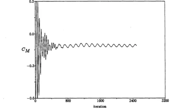
solution. The pitching moment coefficient and the location of vortex breakdown are compared with experimental data measured by Hummel and Srinivasan, with which fairly good agreement is seen in cases in which the location of breakdown is over the wing. A series of unsteady calculations involving a pitching delta wing were performed. The use of the acceleration technique is validated. A hysteresis in the normal force is observed, as in experiments, and a lag in the breakdown position is demonstrated.

Thesis Supervisor: Earl1 M. Murman,

(3)

Acknowledgments

Sometimes a scream is better than a thesis.

Ralph Waldo Emerson

There have been many times during the past five (three, sir) ... three years that could have driven me to scream. I would like to thank all those who have prevented me from needing to do so. First and foremost is my advisor, Earll Murman, who helped me through a thesis that was more (or at lest seemed) trouble-ridden than most. I am also grateful to my other committee members, MArten Landahl and Mike Giles, for their insightful comments and last-minute intercontinental discussions. In addition, Mark Drela helped me understand the practical aerodynamic aspects of this work. This thesis also owes a lot to Liz Zotos, departmental graduate administrator. I would also like to thank Lori Martinez, for being such a nice person, and for always maintaining a supply of interesting food items for public consumption.

I would also like to thank my colleagues at the Cluster, first among them Dana Lindquist and Dave Darmofal, fellow long-term survivors and system maintainers; and my office-mates Yannis Kallinderis, Sandy Landsberg, Brian Nishida, and Eric Sheppard. Life here would have been much grimmer without the Thursday evening custom of trips to the Cambridge Brewery. I'd like to thank Bob Haimes, Gerry Guenette and Mike Giles for starting this tradition.

I'd also like to thank the residents of Jiirgendiir and Ikayama, and the members of the West Somerville Alumni Association - namely Rob, Laura, Susie, Phil, Brian, Eon, Dave, David, Charles, John, Donna, Francis, Kate, Mike, Derrick, and Glenn - for being cool neighbors; and other members of the midnight Illuminati crowd, for helping me get less sleep :)

And last, but by no means least, I owe a lot to my parents, for always believing that I could finish this, even when I didn't believe it myself.

This research was supported by Air Force Office of Scientific Research contract num-ber AFOSR-89-0395A, monitored by Dr. L. Sakell; and by the McDonnell Aircraft Company, under MDC/MDRL IRAD Sponsorship. The mesh generation system was provided by Jaime Peraire of the Imperial College of Science, Technology, and Medicine, London, England, and Ken Morgan of the University College of Swansea, Wales. Three-dimensional visualization was performed using VISUAL3, developed by Robert Haimes of MIT.

(4)

List of Figures

1.1 Classification of delta wing flow regimes . ... 17

1.2 Leading edge vortex structure ... 18

1.3 Fine mesh conical flow solution from Powell, possibly showing the viscous sheath .... ... ... .. ... ... ... ... ... .. 19

1.4 Flow visualization of vortex breakdown over a delta wing . ... 21

1.5 Flow conditions leading to vortex breakdown ad vortex lift-off in incom-pressible flow ... 22

1.6 Measured aerodynamic coefficients on a pitching delta wing ... . 23

3.1 Section of a triangular mesh ... ... 37

3.2 Tetrahedral cell nomenclature ... ... 38

3.3 Triangular area coordinates ... 41

3.4 Normal and tangent vectors at a node on the boundary . ... 52

3.5 Section of an unstructured mesh, with node-to-face-center edges ... . 58

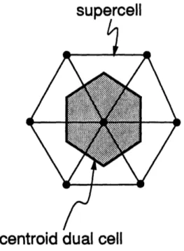
3.6 Supercell and centroid dual cell of a node . ... 65

3.7 Refinement of a triangle ... 74

(9)

4.1 Smooth and linear interpolation in one dimension, and linear

interpola-tion error ... ... 80

4.2 Jagged interpolation of a smooth function in two dimensions. ... . 81

.4.3 Total pressure loss in a Lamb vortex: interpolation of the analytic solution. 82 4.4 Delta wing geometry. ... 83

4.5 Surface triangulation of delta wing for coarse mesh... 84

4.6 Slice through coarse and adapted meshes at 70% of root chord. ... 85

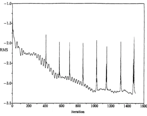
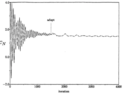
4.7 Iteration history of root mean square of state vector for ae = 420 case. . 86 4.8 Iteration history of coefficient of normal force for a = 420 case. ... 87

4.9 Stationary wing normal force coefficient versus angle of attack, without adaptation ... ... 88

4.10 Stationary wing normal force coefficient versus angle of attack, with adap-tation ... . . . .... . ... 89

4.11 Stationary wing pitching moment coefficient versus angle of attack. ... 90

4.12 Iteration history of coefficient of pitching moment for a = 320 case. ... 90

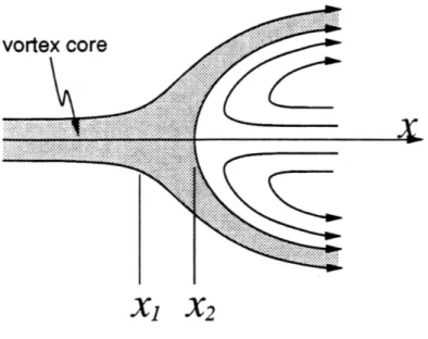
4.13 Vortex breakdown location versus angle of attack. . ... 91

4.14 Detail of the region of vortex breakdown, showing two criteria for break-down location ... 93

4.15 Iteration history of vortex breakdown position for a = 320 case... 94

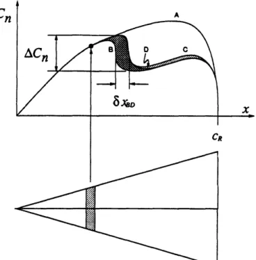
4.16 Change of normal force to to motion of vortex breakdown... 95

4.17 Variation of local lift with axial position, at a = 380. ... 97

(10)

4.19 Computed density variation at z/cR = 0.90, for a = 20.50 ... 100

4.20 Density variation at z/cR = 0.90, for a = 20.5', from Ekaterinas and Schiff.101

4.21 Computed entropy variation on coarse mesh at z/cR = 0.70, for a = 20.50.102

4.22 Computed entropy variation on adapted mesh at z/cR = 0.70, for a = 20.50.102

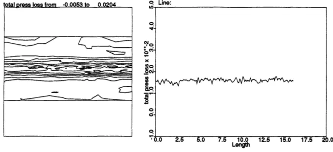
4.23 Computed total pressure coefficient variation along the vortex axis on

adapted mesh, for a = 20.50. ... 104

4.24 Pressure on the upper surface of the wing, at a = 320, on adapted mesh. 105

4.25 Computed axial velocity variation on adapted mesh at z/cR = 0.90,

for a = 320... 106

4.26 Axial velocity variation at z/cR = 0.90, fort a = 320, from Ekaterinas

and Schiff ... 106

4.27 Vortex breakdown region, showing the vortex core and the region of re-versed flow, for a = 320, on adapted mesh ... 107

4.28 Pressure on the upper surface of the wing, at a = 420, on adapted mesh. 109

4.29 Vortex breakdown region, showing the vortex core and the region of re-versed flow, for a = 420, on adapted mesh ... 110

4.30 Computed variation of axial velocity through the vortex core, for a = 420,

on adapted mesh ... ... 111

4.31 Computed variation of entropy through the vortex core, for a = 420, on

adapted mesh. ... 111

4.32 Flow visualization of the bubble type of vortex breakdown in swirling pipe flow, showing downstream reformation of the vortex core, from Sarpkaya. 112

4.33 Computed variation of axial velocity through the vortex core, for a = 420,

(11)

4.34 Computed variation of entropy through the vortex core, for a = 420, on

coarse m esh ... 113

4.35 Variation of wing normal force versus angle of attack during pitching motion, showing effect of local time steps. ... ... . 115

4.36 Variation of vortex breakdown position versus angle of attack during pitching motion, showing effect of local time steps. . ... 116

4.37 Variation of wing normal force versus angle of attack during pitching motion, compared with stationary wing computations. . ... 117

4.38 Variation of vortex breakdown position versus angle of attack during pitching motion, compared with stationary wing computations. ... 118

4.39 Determination of phase delay of two signals that vary with the same

frequency. ... 119

4.40 Variation of vortex breakdown position versus angle of attack during pitching motion, compared with ideal phase lagged sinusoidal motion. . 120

A.1 Propagation of physical and numerical waves in a region of local time steps.131

B.1 Vortex shedding behind a flat plate normal to the incoming flow. ... 134

B.2 Triangular mesh around the flat plate, with a closeup of the region near

the plate ... ... 135

B.3 Contours of pressure in the flow past the flat plate ... 136

B.4 Coefficient of pressure on the surface of the plate... . 136

B.5 Contours of time step in the region of local time steps, for a time step

acceleration factor of 5. ... .. 137

B.6 Time history of drag coefficient on the flat plate at different values of the global time step acceleration factor. ... ... . . . 138

(12)

List of Tables

2.1 Nondimensionalization of flow quantities . ... 34

2.2 Nondimensional parameters ... 34

2.3 Nondimensional aerodynamic coefficients . ... 34

3.1 Nodal memory usage for flow solution procedure . ... 69

3.2 Cellular memory usage for flow solution procedure . ... 69

3.3 Memory usage for adaptive refinement procedure . ... 78

(13)

Nomenclature

Refer also to sections 2.4 and 2.5.

Roman symbols

a speed of sound

a fluid acceleration

b wing span

b unit binormal vector

c wing chord

cR wing root chord

IE wing mean aerodynamic chord cp coefficient of pressure

CPo coefficient of total pressure C characteristic vector C, chordwise coefficient of lift CD coefficient of drag

CL coefficient of lift

CN coefficient of normal force CM coefficient of pitching moment D artificial dissipation

D wing drag

E second difference operator e internal energy per unit mass E total internal energy per unit mass f time step acceleration factor

F flux vector

F, G, H Cartesian components of flux vector

h total enthalpy

h, total rothalpy

J Jacobian

J-1 inverse Jacobian

k reduced frequency

K: nondimensional pitching rate

L wing lift

£ Lagrangian function

M mass matrix

(14)

M Mach number

n surface unit normal vector

n surface normal coordinate

N wing normal force

N interpolation function

N test function

Nc number of mesh cells

NE number of mesh edges

Np number of mesh nodes

p fluid static pressure

P0 fluid total pressure

q fluid speed

Q

a quantity

ro position vector

r not quite the spectral radius

R residual vector

Rx, Ry, Rz residual matrices Rin, Rout Riemann invariants

s entropy

s shock smoothing switch

S face area vector

S source vector

t unit tangent vector

t time

t wing thickness

u, v, w Cartesian components of fluid velocity

V fluid velocity

U state vector

V cell or supercell volume

z, y, z Cartesian coordinates

Greek symbols

fa angle of attack

C1, ... Runge-Kutta coefficients

0angle of yaw

P wing leading and trailing edge bevel angle

7 ratio of specific heats

At time step

APo total pressure loss

E2, E₄ empirical coefficients of second- and fourth-difference smoothing terms

eq weights for fourth difference smoothing terms

(1, C2, C3, C4 tetrahedral volume coordinates

A Courant-Friedrichs-Levy number

(15)

Greek symbols

A characteristic matrix

A wing leading edge sweepback angle

p fluid density

w rotational velocity

fl angular frequency

and superscripts free stream

in absolute (inertial) frame of rel mesh node quantity

tensor indicial notation in surface normal direction in rotational (noninertial) frame at solid wall

mesh cell quantity mesh face quantity

nondimensionalized quantity ference of reference Subscripts

()oo

()

()r

(),

()C

()F

()*

(16)

Chapter 1 Introduction

We never see the beginning. We come in after the lights have gone down and try to make sense of what we have seen.

Neil Gaiman

The Sandman

The latest generation of high performance fighter aircraft are being designed to be capable of extreme maneuvers, which require the aircraft to fly at very high angles of attack that previous aircraft were designed to avoid. At these extreme angles of attack, the leading edge vortex that forms above the aircraft's delta wing suffers breakdown, which degrades the aircraft's handling characteristics. In this section, the delta wing leading edge vortex, and the phenomenon of vortex breakdown are described, and a set of wind tunnel experiments of a pitching delta wing are summarized. In addition, previous numerical simulations involving leading edge vortex flows, and vortex breakdown, are mentioned.

1.1 Background

The aerodynamics of delta wing flows is of great interest for two main reasons. The first is that when a symmetric and stable set of vortices forms, the wing experiences an increase in lift and aerodynamic moments, leading to enhanced aircraft maneuverability. The second is that an asymmetric or unstable set of vortices can cause a loss in lift and

(17)

500 0 40 -3I I 0 N

MN

Figure 1.1: Classification of delta wing flow regimes [53]

a strong rolling moment, even with no angle of yaw. Either of these consequences can lead to disaster for a maneuvering aircraft.

Stanbrook and Squire [76], and later Miller and Wood [53], classified the various regimes of flow behavior around a delta wing. The classification system of Miller and Wood is summarized in figure 1.1, in terms of the Mach number and angle of attack normal to the leading edge of the wing. These quantities are defined to be

MN

=

Moo cos A 1 + sin

2

ata

2

(1.1)

aN = tan- tana (1.2)

cos A

in which A is the sweep angle of the leading edge of the wing. The regime at low normal Mach number and moderate angle of attack is that which involves separation at the leading edge, and is the regime in which the flows of interest in this thesis occur.

(18)

VISCOUS SUBCORE

INVISCID CORE

VISCOUS SHEATH

FEEDING SHEET

SECONDARY VORTEX

Figure 1.2: Leading edge vortex structure

1.1.1 Leading Edge Vortex Structure

At sufficiently high angle of attack, the fluid flow will separate at the leading edge of a delta wing, resulting in the formation of a large pair of primary vortices above the lee side of the wing. A large body of experimental investigations of the leading edge vortex structure indicates that the vortex can be divided into three parts, each with its own distinctive properties. The structure is shown in figure 1.2. The feeding sheet, or umbilical shear layer, is a viscous thin shear layer emanating from the leading edge of the wing. The vortex itself has two parts. The outer core is a nearly inviscid, rotational region of mostly conical flow. Towards the center of the core the axial velocity is seen to increase dramatically. At the center of the core is the viscous subcore, at the outer edge of which the swirl velocity reaches a maximum, and the axial velocity continues to increase to a maximum at the axis. At the center of the viscous subcore the swirl velocity must vanish. The difference between maximum swirl velocity at the edge of the subcore and zero on the axis causes viscous dissipation which is largely independent of Reynolds number. In addition, Lee [42] describes a model, based on experimental data gathered by Verhaagen and van Ransbeeck [84], in which the rotational core is separated from the external, irrotational flow by a viscous shear layer called the viscous sheath,

(19)

me 1.10 a 10* Dm0 Am 5T 256 x 256 Total pressure los

0.7S INOS .aesO3.O1 0.45

f/a

0.80

0.15 0.,, 3... ass 0.00 -0.1 0.0 0.00 0.15 0.80 0.46 0.00 0.75 0.90 s1.05 1.20 he/

Figure 1.3: Fine mesh conical flow solution from Powell [64], possibly showing the viscous sheath.

which is formed as the feeding sheet rolls up and intersects with itself. Conical flow Euler solutions by Powell [64], one of which is shown in figure 1.3, also provide evidence for the existence of the viscous sheath. Due to the use of the Euler model, the effects of viscosity upon the solution in figure 1.3 are due only to the artificial dissipation and truncation error.

The flow on the leeward surface of the wing is accelerated due to the proximity of the vortex, resulting in a region of lower pressure which increases the lift and pitching moment of the wing. A secondary vortex forms due to boundary layer separation in the adverse pressure gradient as the fluid moves outboard from the pressure minimum directly beneath the primary vortex. Similarly, a tertiary vortex can also appear due to separation beneath the secondary vortex. Simulation of the secondary and tertiary vortices requires the inclusion of viscous effects. The characteristics of the secondary vortex has been shown to affect the structure of the primary vortex in transonic flow conditions [54], but not in supersonic flow [50].

Some experimental investigations into the characteristics of delta wing flow were per-formed by Earnshaw [16], Hummel [28], Verhaagen and Kruisbrink [85] and Verhaagen

(20)

and van Ransbeeck [84], who measured velocity and pressure in the region of the vortex, and Fink and Taylor [19], who studied the variation of total pressure. More recently, Kjelgaard and Sellers [37, 36] and Roos and Kegelman [70] performed exhaustive flow field surveys.

The numerical solution of delta wing flows can sometimes be simplified by use of the conical assumption, in which flow quantities are taken to be constant on rays emanating from the apex of the wing. This simplification is only valid for supersonic flow of an

inviscid fluid around a sharp edged wing of a suitable shape. Powell [64] performed a

study of leading edge vortex flows with the use of embedded structured grids to increase resolution. Batina [7, 5] formulated and solved the conical Euler equations using an unstructured mesh of triangles, and adaptive refinement, and Kandil and Chuang [35] used the conical model to study the unsteady flow that results from a rolling wing.

Fully three-dimensional solutions of delta wing flow are necessary in situations in which streamwise variations occur. Rizzi et al. [68, 55, 67] have performed numerous calculations, particularly for transonic flows. Melton [51] performed adaptive compu-tations in three dimensions using hexahedral cells, and Borsi et al. [10] made use of adaptation using a mesh of tetrahedral cells. In addition, in the absence of vortex breakdown simpler models can provide accurate solutions. An example is the method developed by Tavares [78] using slender wing theory with an explicit vortex wake.

1.1.2 Vortex Breakdown

Vortex breakdown, also known as vortex bursting, is a phenomenon that was first

ob-served in delta wing flows by Peckham and Atkinson in 1957 [58], and was studied in

detail by Lambourne and Bryer [39]. It occurs when a vortex is subjected to a

suffi-ciently strong adverse pressure gradient. The basic features of vortex breakdown are a sudden enlargement of the vortex core, followed by a stagnation region on the axis. The

(21)

Figure 1.4: Flow visualization of vortex breakdown over a delta wing

of vortex breakdown can be seen in figure 1.4, from Lambourne and Bryer. The upper vortex is experiencing the axisymmetric "bubble" type of breakdown, while the lower vortex is undergoing the asymmetric "spiral" type of breakdown. Breakdown has also been observed [57] to alternate periodically in time between the bubble and spiral types, and Sarpkaya [72] reports forms of breakdown intermediate between the two types. The effects of vortex breakdown are a significant decrease in lift and pitching moment, and a large rolling moment due to the possibility of asymmetric breakdown (such as appears in figure 1.4). The deleterious effects of vortex breakdown increase with the angle of attack of the wing, as the location of breakdown moves forward from the trailing edge.

The flow conditions under which vortex breakdown occurs in incompressible flow are summarized in figure 1.5. The angle of attack at which breakdown appears decreases as the sweep angle A decreases, which is to say, as the wing becomes less slender. For very slender wings, asymmetrical vortex lift-off occurs, in which one leading edge vortex retreats from the wing surface, while the other approaches the wing. This produces an anomalous rolling moment, and can lead to an oscillatory motion called wing rock [56,

(22)

30

a

20

10 - Symmetric Vortices

90 80 70 60 50

A

Figure 1.5: Flow conditions leading to vortex breakdown ad vortex lift-off in incom-pressible flow [63]

Surveys of vortex breakdown in general and proposed theoretical explanations of it are presented by Landahl and Widnall [40], Hall [25], Leibovich [43] and Escudier [18]. Numerical investigation of the breakdown process was first performed by Grabowski and Berger [23] for the axisymmetric breakdown in a swirling pipe flow. Numerical simulations of vortex breakdown over a delta wing have also been reported. Fujii and Kutler [20] possibly captured the onset of breakdown, with more demonstrative calcu-lations being performed by Thomas, Krist and Anderson [80], Hartwich, Hsu, Luckring and Liu [26], Ekaterinas and Schiff [17], Agrawal, Barnett and Robinson [1], Deese, Agarwal and Johnson [15] and Webster and Shang [87]. The bubble type of breakdown was specifically noted by Thomas et al. and by Ekaterinas and Schiff, while Webster and Shang characterized their solution as the spiral type of breakdown.

1.1.3 Pitching Delta Wing

Modern fighter aircraft are being designed to perform extreme maneuvers, known as

"supermaneuvers," which involve flight at very high angles of attack, where vortex

(23)

'4°

O.o

0.0 S. s0.0i . n. ie m 0 0 &0 '.e . i.e ieo s s e i.e me oe

ANGL OF AfTAC(

- 0.0 (S IC 0 ... I 0.03

- 5.0.04

Figure 1.6: Measured aerodynamic coefficients on a pitching delta wing [31, 32] breakdown is likely to occur. Previous aircraft have been designed to remain at lower angles of attack to avoid vortex bursting and wing stall. In order to study aircraft performance in this extreme flight regime, Jarrah [32, 31] analyzed three canonical supermaneuvers and determined that the aircraft dynamics could be represented by either a sinusoidal or a ramp variation of angle of attack. Jarrah then subjected a delta wing in a low-speed wind tunnel to pitching motions with both the sinusoidal and ramp variation, and found a large hysteresis in the unsteady aerodynamic forces on the

wing, as shown in figure 1.6. The hysteresis persisted even at low reduced frequencies at which Jarrah expected to observe quasi-steady flow. Jarrah attributed the hysteresis to a lag in the vortex breakdown, whereby the angle of attack at which the vortex breaks down during the upward motion is greater than the angle of attack at which the vortex re-establishes itself during the downward notion. Experiments by Thompson, Batill, and Nelson [81] also indicate the lag in burst location. It is the goal of this work to simulate the unsteady flow around a pitching delta wing and study the behavior of vortex breakdown in this flow. Jarrah and Thompson et al., both found the effect of

Reynolds number on this flow to be weak, so that the Euler equations are adequate to simulate the flow around a sharp-edged delta wing. The unsteady flow around a pitching wing for very small amplitudes of motion was studied by Kandil and Chuang [34].

(24)

1.2 Validity of the Euler Equations

In general, there are two conditions for the validity of the Euler equations for modeling delta wing flows. First, the wing geometry must have a sharp leading edge to provide a Kutta condition for flow separation, and second, the flow solution algorithm must provide a dissipative mechanism to bring the swirl velocity to zero at the vortex core. The wing geometry used for all computations in this thesis has a sharp leading edge, and the artificial dissipation added to the flow solution scheme serves the latter purpose. Experimental investigations indicate that a changing Reynolds number does not affect the structure of the primary vortices [37] or the lift variation with angle of attack [70]. There is also evidence [72] that in the high Reynolds number limit the behavior or vortex breakdown also is independent of Reynolds number.

1.3 Thesis Summary

The goal of the present research is the application of adaptive refinement via mesh-point embedding to the solution of the unsteady inviscid flow around a pitching sharp-edged delta wing. The main body of the thesis is divided into three parts. In chapter two, the governing equations for the flow of an inviscid, ideal gas, the Euler equations, will be presented in an inertial reference frame, and transformed into a rotating reference frame fixed to the wing. Also, suitable physical boundary conditions will be discussed. In chapter three, the procedure for solving the Euler equations numerically will be de-scribed. This includes the spatial discretization by means of the Galerkin finite element method, the artificial dissipation with the Holmes-Connell extension, the temporal in-tegration procedure, the implementation of the boundary conditions, and a detailed description of the adaptive refinement method. In chapter four, stationary and pitching wing flow solutions will be discussed and interpreted. Ultimately, some conclusions will be drawn and some recommendations for further work will be made.

(25)

Chapter 2 Governing Equations

Fluid dynamics is much less interesting if it is treated largely as an exercise in mathematics.

From the point of view of a 'pure' scientist concerned only with basic laws, there seems to be little need to go further.

The set of governing equations is much too complicated for a direct mathe-matical approach to be feasible.

G. K. Batchelor

In this chapter, the governing equations for inviscid, compressible flow in an iner-tial reference frame are derived, and appropriate choices for nondimensionalization and boundary conditions are described. In addition, the equations for the flow are trans-formed into a non-inertial reference frame, which is specialized to rotation about a fixed center.

2.1 Inertial Frame of Reference

The Euler equations are a system of partial differential equations that describe the behavior of an compressible, inviscid, non-conducting fluid. They are derived from the integral form of the laws of conservation of mass, momentum, and energy, in an inertial frame of reference.

(26)

For an arbitrary fixed control volume V, the law of conservation of mass can be expressed as

- pdV = -j p(ujnj)dS (2.1)

where p is the density, uj is the fluid velocity, expressed using indicial notation, and nj is the outward-pointing unit normal vector at the surface of the control volume. This states that the rate of change of the mass of the fluid in the control volume is equal to the transport of mass across the control volume boundary, OV. Gauss' divergence theorem is used to transform the surface integral into a volume integral over V. Then,

by requiring the resulting integral equation to hold for any infinitesimal control volume,

the differential form of the law of mass conservation is found to be

ap

a

+

-

(pu) = 0

(2.2)

atazt

which holds everywhere that the flow quantities are continuous and differentiable. At discontinuities, only the integral form is valid.

The integral form of the law of conservation of momentum can be written as

-f

pu dV = - pui (ujnj) dS -

pni

dS (2.3)

Tf , 8v v

where p is the static pressure of the fluid. The index i spans the three equations, and the repeated index j indicates summation. These equations state that the momentum of the fluid within the control volume is changed by the transport of momentum across the surface, and by the action of fluid pressure on the surface OV. Again, the divergence theorem is used to transform the surface integral terms. The differential form of the momentum equation,

(

a

(P-uL) + i (piuj + p) = 0 (2.4)

results.

Again,

form is not valid at flow discontinuities.

the

differential

(27)

The integral form of the law of conservation of energy can be written as

-f pE dV = - pE (ujnj) dS - uj (p nj) dS

t v ev fav (2.5)

where E is the total internal energy per unit mass. This states that the energy within the control volume is changed by the transport of energy across the surface, and by the work done by the action of the fluid pressure upon the surface of V. By application of the divergence theorem, the energy equation can be transformed into its differential form,

E) +

([pE + p]

(pE) + ([pE + p

uj)

= o (2.6)

which is only valid in continuous regions of the flow.

Since the three conservation laws have analogous terms, they can be grouped to-gether to form a system of equations,

9U

OF

S+-7 +

Ot

Oaz

where the state vector U is

U =

and the Cartesian components of the flux

F =

pu

pU2 + p puV

puw

puh f

OG

OH

+ -

= O

Dy

Oz

P Pu pv pw

pE

vector, F,

pv

putv

v2 + pvw

pvh

(2.7) (2.8) G and H are pw pow pw2 +p pwh

(2.9)

(28)

compo-nents, u, v and w. The quantity h is the total enthalpy, defined to be

p

h=E+

The system is closed by the equation of state for a perfect gas,

p= (y-1) pe,

(2.11)

where e is the internal energy per unit mass, which is defined by the thermodynamic relation

E = e + (R 2 + 2 + 2), (2.12)

and 7 is the ratio of specific heats, cp/c,.

2.2 Rotating Frame of Reference

To express the Euler equations in a moving, non-inertial frame of reference, in which derivatives are denoted by a prime superscript, substitute the following transformations for the derivatives of an arbitrary scalar and an arbitrary vector into the Euler equations:

DQ

D'Q

Dt Dt'

DQ

D'Q

+

oDt'x

Dt Di'

or, expanding the total derivatives:

OQ

O'Q

ot

-vt.VQ

-t '-

_{Q.vQ +}

_-v

t

_xQ

Ot

at'

where

(2.15)

is the transformation velocity from the absolute frame of motion, in which the fluid velocity is 'v, to the moving, relative frame, in which the fluid velocity is v,. The

(2.10)

(2.13)

(2.14)

(29)

relative motion can have both a translational velocity, to, and a rotational velocity about a fixed point, from which the position vector ' is referenced. The rotation need not be steady. When the transformations 2.14 are substituted into the Euler equations (2.7, 2.8, 2.9), the system gains a source term, S, which contains terms related to the motion of the frame:

O'U

OF

OG

OH

+

+ +

= S.

at'

Be

By

8z

(2.16)

Also, several of the primitive variables have changed meaning, so that the state vector is now U = P pu, pv, pw, pE, (2.17)

and the flux vector is

pu, Pur + p pu,.wv,. pu,.h, pVy pur v, pVr + p Ptw,. pv,.h,. put w, pw +p pw,h, (2.18)

This is the same form of the unsteady Euler equations as used by Kandil and Chuang [35, 34]. The fluid velocities are now measured in the relative frame of reference, and the total energy and enthalpy are replaced with new quantities, which are related to the quantities of the absolute frame by

E, = E-v .t -h, = h- v -vt.

(2.19)

(2.20)

The quantity h, is called the total rothalpy, and is constant in steady flows in a rotating reference frame, as is the total enthalpy in a nonrotating frame. The source term S has

(30)

the complicated form 0 -pat_ S = -paty (2.21) -patz -p

do

W

+ VO(WXVa)} where D, D'i, at = (2.22) = ao + xr'F + 23x + W x(xrF) (2.23)

is the relative acceleration of the two frames, having linear, angular, Coriolis, and cen-tripetal terms, respectively.

The cumbersome form of the energy source term is reduced by restricting the form of the transformation velocity. In this case, the motion is required to be purely rotational, so that the translational terms, io and do, vanish, giving a source term with the form

0 -pat,

= -pat, . (2.24)

-patz

-p f((v + - :

(31)

the angular velocity w is equal to the pitch rate, &. The source term now can be written 0 -p(dz + 2ww, - w2X) S = 0 (2.25) -p(-Cx - 2wu, - w2z) -p

{(uz

- Wz) + w(X2 + Z2)}

where z and z are measured from the center of rotation. In addition, the variation of the angle of attack, and thus the rotation rate w, is taken to vary sinusoidally with an angular frequency of a. Specifically, the angle of attack varies as

a = ao + !Aa(1 - cos at) (2.26)

The rotation rate is then

w = dAa sin t, (2.27)

which has a maximum value of

wmax = at. (2.28)

In addition, the angular acceleration is

j = f2 Aa cos nt. (2.29)

The energy source term in equations 2.24 and 2.25 vanish if the rotation is steady, as occurs in most turbomachinery and rotorcraft flows. However, the Coriolis and centripetal contributions to the momentum source terms remain.

2.3 Physical Boundary Conditions

There are three different physical boundary conditions to apply to the Euler equations. The implementation of these boundary conditions is discussed in section 3.3.

(32)

2.3.1 Solid wall

At a solid wall, no flux is permitted through the surface. This condition is written as

u.n= 0 (2.30)

where n' is the unit vector normal to the surface. This condition also applies at symmetry surfaces.

2.3.2 Kutta condition

Since there is a multitude of solutions for the flow around an arbitrary body, some condition must be imposed to collapse to a single solution. For the flows that will be considered in this thesis, the Kutta condition can be applied at sharp edges of the wing to fix the lift. For sharp-edged delta wings, both the leading and trailing edges are treated this way.

2.3.3 Far field

In the far field, the flow should approach a uniform free stream in the inertial refer-ence frame. By use of equation 2.15, this is transformed in the rotating frame into a free stream with time-varying solid body rotation imposed. Since it is impossible to model variations at infinity using the numerical methods described in this thesis, the implementation of this boundary condition will be the most mathematically complex.

(33)

2.4 Nondimensionalization

It is often desirable to make the Euler equations dimensionless to solve them numerically. This makes the problem independent of the choice of units, clarifies the scales relevant to the problem, and can reduce the sensitivity of the solution procedure to numerical round-off errors. The reference parameters used are the freestream density, p,, the freestream speed of sound, ao, and a characteristic length. In this thesis, the wing root chord, cR, is chosen as a length scale. The nondimensionalization factors for some flow quantities are listed in table 2.1. There are three important nondimensional parameters, which appear in table 2.2. The freestream Mach number, M,, measures the importance of compressibility, while both the reduced frequency, k, and the nondimensional pitch rate, K, both measure the importance of unsteady effects. The reduced frequency measures the frequency of unsteady effects, and the nondimensional pitch rate measures the amplitude of unsteady effects. The latter two parameters are related by

2K

k - (2.31)

Aa

where Aa is the range of angle of attack variation during the unsteady cycle. The flows in this thesis have a low Mach number in the subsonic range. A flow with a low reduced frequency is referred to as quasi-steady, meaning that the evolution of the flow with

time is a succession of steady flows, with varying parameters.

The form of the Euler equations is unchanged by this nondimensionalization, but the free stream boundary conditions are altered. With this set of reference parameters, the freestream state vector takes the form

P 1

pu

M. cos a cos / - wz

pv

=

M. sin

(2.32)

pw

M, sin a cos I + wx

(34)

Table 2.1: Nondimensionalization of flow quantities

Table 2.2: Nondimensional parameters

Coefficient Symbol Dimensional Nondimensional

N N*

normal force CN 2 MAR

pooqooS AR L L* lift CL 2 1 Spqoo S I8 MAR D D* drag CD 1 2 1 2 SpoooqS &M AR M M* pitching moment CM 1 2 S TpooqaSE c MAR

Table 2.3: Nondimensional aerodynamic coefficients

Quantity Reference Freestream Value

P Poo 1

u, v, w, a ao M. cos a cosp -wz, M, sin i, M. sin a cos 3

+

w , 1

E, h

a

o

+ + 1 p pa, 1/l z, y, Z CR t CR/ao w,

n

aoo/CR -, 2Mook N, L, D

pac2

M poa ooCR PooaOO R

Parameter Symbol Definition

freestream Mach number Moo q

aao

reduced frequency

k

CR

2q,

(35)

in which M is the freestream Mach number, a and 3 are the angles of attack and yaw, respectively, and w is the rotation rate.

The forces that act on a wing are characterized by the dimensionless aerodynamic coefficients of normal force, lift, drag and pitching moment. The definitions of these coefficients, in terms of both dimensional and dimensionless quantities, are given in ta-ble 2.3. The forces are normalized by the freestream dynamic pressure and the wing area. The pitching moment has an additional normalization factor, ,, the mean aerody-namic chord of the wing. For a triangular wing, this has the value of two-thirds of the wing root chord. In addition, these formulae assume that the forces are due to the effect of the entire wing. When simulating flows about a wing at zero angle of yaw, one can take advantage of the symmetrical nature of the problem to compute a solution within a domain of half the size. In such a case, the aerodynamic force coefficients must be doubled to obtain their values for the entire wing.

2.5 Auxiliary Quantities

The following is a list of auxiliary quantities, defined in terms of the primitive variables:

Quantity

Local flow speed: Local speed of sound: Local Mach number:

Total pressure: Total pressure loss: Entropy: Definition q = V 2 + v2 + W2 V P

M =q

a Po = 1

+O

Po Apo = 1 Freestream 1 Moo 1 + M2 .

0

(36)

Chapter 3 Numerical solution procedure

God made integers, all else is the work of man.

Leopold Kronecker

Jahresberichte der Deutschen Mathematicker Vereinigung, bk. 2

In this chapter, the numerical solution method for solving the governing equations is derived. The procedure used is a finite element method based on a mesh of tetrahedral cells. Also, the temporal integration procedure is discussed, along with the implementa-tion of the physical boundary condiimplementa-tions and the numerical smoothing procedure. The chapter also includes a description of the adaptive refinement procedure.

3.1 Mesh geometry

The tetrahedral cell is the basis for most of the calculations described here. The faces and nodes of a cell are numbered such that node j is opposite face j. Thus each face is defined by the three nodes with different numbers. The outward-pointing area normal S of each cell face is frequently used. It is constructed by taking the cross product of any two edge vectors of the face, with the requirement that it point outwards. Thus,

(37)

supercell of node 1

Figure 3.1: Section of a triangular mesh

S

1

=

(y32 42

-

z

32

y

42

)

s'= (32 X X42) S2( = - a~32 z42) (3.1) 5

₁

₌

₍

32

y

42

-

Y3242)

s522 = 4131 - z4 1 3 1) S2 = (41 X X31) S, 2 = (zI 1 - (3.2) Sz₂ = -(X41Y31 - Y41X31)

S

,3

=

(Y21z41 - z

21

y

41

)

S3 = (X21 X 41) Sys = (z₂1 41 - X2 1 4 1) (3.3) Sz3 = (21Y41 - Y21X41) S, 4 (= ( 3 1Z21 - z3 1Y2 1) S4 = ( 31 X 21) S 4 = (z3 1XZ2 1 - zXz21) (3.4) Sz4 = I( 3 1Y2 1 - Y31Z21)

where zij = - j, yij = y - yj and zij = zi - zj. Although it is far from obvious based

on the above formulas, the vector sum of the areas of the four faces of a tetrahedron is zero. This is a general result for a closed surface.

The union of all cells that contain a node is called the supercell of that node, as represented for the analogous two-dimensional situation in Figure 3.1. The volume of the supercell of node i is the sum of the volumes of the cells of which node i is a vertex.

(38)

node 3

face 4

node 4

node 1

Figure 3.2: Tetrahedral cell nomenclature

The volume of a tetrahedral cell is

221 Y21 Z21

Vc= 2₃₁ Y31 Z31

24 1 Y41 Z4 1

6 (X21y31z41 + Y21z3 1 41 + z21X3 1y41

-z21Y3141 - 21iz31Y41 - Y2 1z 3 1 4 1)

where

xj = xi - xj

is the edge vector between the ith and jth nodes of the tetrahedron. The vertices of the cell are numbered so that nodes 1, 2 and 3 are in a counterclockwise orientation when viewed from node 4. A single tetrahedral cell is seen in figure 3.2, showing the node and face numbering, and a typical face area vector.

The boundaries of the mesh are arranged so that the nodes are numbered in the counterclockwise direction when viewed from the interior of the computational domain. The surface normal at a boundary node is the area-weighted average of the normals of

(3.5)

(3.6)

(39)

the boundary faces that contain the node. The boundary normal is the cross product of two edge vectors that yield the correct direction. Thus,

S 1 ( 21 x X_31)= 2 (X32 X X1₂)= 2( 13 X X23)

s

=

F

(y21z31 - z21Y 3 1) S 2 (3.8) = = (z21s31 - Z21z31)

S

=

(X2131

- Y21 3 1)

All boundary normals point into the computational domain.

3.1.1 Mesh Generation

Tetrahedral meshes are generated by the advancing wavefront method, using a mesh generator developed by Peraire, et al. [59, 61]. A three-dimensional mesh is generated in two steps. First, a surface mesh, composed of triangular elements, is generated. Then, using the surface mesh as an input, a volume mesh, composed of tetrahedra, is generated in the flow field. Mesh generation begins with the assembly of a front of triangles, which is initialized to be the surface mesh. Then, every triangle is examined, and a tetrahedron is created with the triangle as a base, and having a height calculated according to a mesh point spacing function, which is controlled by the user. The node at the peak of the tetrahedron will be an existing node of the mesh if a suitable node exists, or, if not, it is created. The original triangle is then removed from the front. The procedure continues until the front does not contain any triangles.

3.2 Finite element method

Spatial discretization is by means of the Galerkin finite element method with tetrahedral cells. The mass matrix is lumped, resulting in a scheme identical to the cell-vertex finite volume method in which control volume for node i is the supercell of the node.

(40)

However, the finite element and finite volume methods lead to different discretizations when viscous effects are modeled. A detailed discussion of the finite element method can be found in Cook [12], although with an emphasis on applications to structural mechanics.

The basis of the finite element method is that the spatial variation of the state and flux variables is represented in terms of nodal values of these quantities, Ui(t), Fi(t),

Gi(t), Hi(t) and Si(t), and interpolation functions Ni(z, y, z), so that

U(Z, y, z, t) = N(z, y, z) Ui(t) F(z, y, z, t) = Ni(, y, z) Fi(t)

G(,y, z, t) = Ni(z,y, z) Gi(t) (3.9)

H(o,y,z,t) = Ni(z,y,z) Hi(t)

S(z, y, z, t) = Ni(z, y, z) Si(t)

in which the repeated index i indicates a sum over the nodes of the mesh. The in-terpolation functions Ni have a value of unity at the node i, and a value of zero at all other nodes. The sum of all the interpolation functions must be unity, so that a uniform field results when all the nodal quantities are equal. A distinction of the finite element method, as opposed to other interpolation methods, is that the global inter-polation functions are a piecewise combination of local interinter-polation functions, one per cell. This means that the variation of a quantity inside a cell is a function only of the nodal quantities and interpolation functions associated with the nodes of that cell. The local interpolation functions are taken to be zero outside the cell. The superscript C is used to represent a quantity associated with a cell.

(41)

A = A

+

A2 + A3

I

= _P₌_P(C1,_{C2,9 3)}

AA 3

2

Figure 3.3: Triangular area coordinates

3.2.1 Interpolation functions

The local interpolation functions used here are trilinear. They are defined in terms of a local coordinate system, which is the set of tetrahedral volume coordinates C1, C2,

C3 and

C4,

which are shown for the analogous two-dimensional situation in Figure 3.3. An arbitrary point P divides the tetrahedron into four sub-tetrahedra. The volume coordinates are defined as ratios of the volumes of the sub-tetrahedra to the volume of the entire tetrahedron:

V1 V₂ V₃ V4

C1

_VC'

2

_{V '}

3

_VC'

C4 =(3.10)

_V(.

Since Vc = V

+

V2 + V3 + V4 these coordinates are not independent, but satisfy the relation

(1

+

(2

+

4 =

1. (3.11)

Therefore C4 is replaced by 1 -

C(

- C2 - (3. The volume coordinates each have a value of unity at the node with which they are associated, and a value of zero at the other three nodes of the tetrahedron. Since these are the properties desired in a set of interpolation functions, the interpolation functions are taken to be exactly the volume coordinates,

(42)

so that

NC = (2 (3.12)

N4C = (4 = 1 - 1 -C2 -3

The local coordinates are often referred to as natural coordinates.

3.2.2 Spatial Discretization

The discretization of the Euler equations proceeds as follows. First, the interpolated representations of the state, source and flux quantities (Eqn. 3.9) are substituted into the Euler equations, giving

NidU NSi Fi - ON i - NHi (3.13)

dt

az

y

Oz

in which indicial notation is again used. Note that this is a single vector equation, not a system of equations. The interpolation imposes a form on the solution that is unlikely to satisfy the Euler equations at every point in the field. Therefore it is necessary to recast the equations in the weak form by projecting them onto the space of

test functions Nj and integrating over the solution domain. The test functions, which

are again associated with the mesh nodes, roughly correspond to control volumes over which the integral equations are satisfied. In the Galerkin approach, the test functions are identical to the interpolation functions for the same node. We now have a set of equations

dU

raN.

ON- ONN-I

i

NNjdV

= S

NiNjdV-F

-NdV-Gf

'

NdV

-

-N

dV

dt a y z

(43)

in which the repeated index i indicates summation over the set of nodes, while the non-repeated index j spans the set of equations. Equations 3.14 can be written as

dU

Mi-

_dt

-

= M jSj - Rx,jFii

-

Ry,ijGi

-

Rz,fijH

(3.15)

in which Mij is the consistent mass matrix, and Rx,ij, Ry,ij and Rz,ij are the residual matrices. These matrices are defined by integration over the entire domain. However, since the interpolation and test functions are defined piecewise with regard to the cells, these integrals can be broken up into a sum of integrals over the individual cells, so that

M'i

=

Jyv

?,= JV

F

zg

= J

NiNj dV

N

_dV

ONi

-- Nj dV

Ny d

Od

(3.16) (3.17) (3.18) (3.19)

It is now possible to write equation 3.15 as

(e MC

dU-cels ' dt

c

S

c

(cells /cells

RX ij) F

2

-The range of summation is the group of cells that supercell of the node.

contain node i,

(3.20)

which form the

3.2.3 Calculation of Matrices

Integration of Equations 3.16 through 3.19 is carried out in the local coordinate

sys-tem (C1, C2, C3). The spatial derivatives of the interpolation functions are evaluated by

the chain rule, as

Adaptive Mesh Euler Equation Computations of Vortex Breakdown in Delta Wing Flow

Adaptive Mesh Euler Equation Computation of

Vortex Breakdown in Delta Wing Flow

David Laurence Modiano

@Massachusetts

/

FEB 17

1993

.,-Adaptive Mesh Euler Equation Computation of Vortex

Breakdown in Delta Wing Flow

David Laurence Modiano

Acknowledgments

Contents

List of Figures

List of Tables

Nomenclature

Q

a quantity

()oo

()

()r

(),

()F

()*

Chapter 1

Introduction

The Sandman

1.1

Background

MN

=

Moo cos A 1 + sin

ata

(1.1)

cos A

f/a

0.80

1.1.2

Vortex Breakdown

Vortex breakdown, also known as vortex bursting, is a phenomenon that was first

ob-served in delta wing flows by Peckham and Atkinson in 1957 [58], and was studied in

detail by Lambourne and Bryer [39]. It occurs when a vortex is subjected to a

a

A

1.1.3

Pitching Delta Wing

Modern fighter aircraft are being designed to perform extreme maneuvers, known as

"supermaneuvers," which involve flight at very high angles of attack, where vortex

1.2

Validity of the Euler Equations

1.3

Thesis Summary

Chapter 2

Governing Equations

2.1

Inertial Frame of Reference

ap

a

+

(pu) = 0

(2.2)

atazt

-f

pni

a

results.

Again,

form is not valid at flow discontinuities.

the

differential

E) +

([pE + p]

uj)

9U

OF

S+-7 +

Ot

Oaz

U =

F =

_{Q.vQ +}

_-v

_xQ