Adaptive loop sensitivity characteristics for a model reference adaptive control system

\ST. OF T ECH/Vol

AUG 10 1961

IBR A R% ADAPTIVE LOOP SENSITIVITY CHARACTERISTICS

FOR A MODEL REFERENCE ADAPTIVE CONTROL SYSTEM

by

Thomas Howard Barrie B. S. E. E. , University of Washington

and

Bradford Wells Parkinson

B. S., United States Naval Academy 1957

Submitted in Partial Fulfillment of the Requirements for the Degree of Master of Science

at the

MASSACHUSETTS INSTITUTE OF TECHNOLOGY June, 1961

Signatures of Authors

Signature redacted

Signature redacted

Certified by

Accepted by

,epartment of Aeronautics and Asr/p Ma2O, 1961

___

Signature redacted

Thesis Supervisor

fSignature

Chairman, Departmenta Committee on Grad ate Students 1955

1%,

ii

ADAPTIVE LOOP SENSITIVITY CHARACTERISTICS

FOR A MODEL REFERENCE ADAPTIVE CONTROL SYSTEM

by

Thomas Howard Barrie Bradford Wells Parkinson

Submitted to the Department of Aeronautics and Astronautics on May 20, 1961, in partial fulfillment of the requirements for the degree of Master of Science.

ABSTRACT

The object of this study was to outline the adaptive loop per-formance as a function of adaptive loop sensitivity, taking into

con-sideration input, initial conditions and operating environment in a model reference adaptive control system, and from these results, determine a method of adaptive loop .design. Primary means of de-termining system performance was analogue simulation with analytic

corroboration in limited areas. From these studies it was found that to determine adaptive loop performance only initial condition

and environment were independent parameters. Based on the know-ledge of adaptive loop performance and input magnitudes a design procedure was outlined.

Because the input magnitude was found to have an over-powering effect on system operations an attempt to reduce this

dependency was made using limiters. The limiters greatly reduced the dependency of the adaptive operation on input magnitude and also sibiplified the design procedure.

Thesis Supervisor: H. Philip Whitaker Title: Associate Professor of

iii

ACKNOWLEDGEMENT

We express our thanks to:

Professor Whitaker, for his stimulating suggestions, criticisms and supervision;

Mr. Allen Kezer, for his instruction onthe use of the GPS analogue computer;

Miss Betty Belknap, for typing the manuscript;

and, last but not least, our wives, Barbara and Jill, who have contributed in full measure their under-standing, patience and moral support throughout the past two years.

All these people have made this task a little less impossible.

"The graduate work for which this thesis is a partial requirement was performed while the authors were assigned by the Institute of Technology, United States Air Force, for graduate training at the Massachusetts Institute of Technology. "

iv

TABLE OF CONTENTS

Chapter No. Page No.

1 Introduction

1.1 Concept of Adaptive Control Systems 1. 2 History and Development

1. 3 The Integral Squared Error Criterion 1. 4 Mechanization of the Adaptive Loop 1. 5 Synopsis of System and Model Used

Description of the Problem Discussion of Results

3. 1 Problem Simulation 2

3. 2 SAL 2Equivalency

3. 3 Linearity of Adaptation with Adaptive Loop Gain

3.4 Instability Regions 2

3. 5 Variation of SAL 2 with Initial Parameter Setting

3. 6 Gain Ambiguities. for 100% Adaptation 3. 7 Variations in Adaptive Loop Sensitivity

with Flight Condition

3. 8 Performance of the Adaptive System Using Limiters

3.9 Extension of Limiter Results to Other Configurations

Conclusions

4. 1 Summary of Adaptive Loop Characteristics 4. 2 Design Procedure

V Appendices A B C D E F G Figures 1 2 3 4 5 6a, b 7 8 9 10 11 12 Block Diagrams Aircraft Characteristics Computer Wiring Diagrams Graphical Results

Analysis of the Adaptive System

Outline of Suggested Areas for Further Study Bibliography Page No. 41 44 45 49 56 60 62

Functional Diagram for a Model Reference

Adaptive Flight Control System 3 Mathematical Block Diagram of a Model

Reference Adaptive Control System 5 Example Mechanization for a Parameter

Control Loop 8

Generalized Block Diagram Showing

Adjustable Parameter 9

2 Block Diagram Representation of SAL 2

Argument 17

2

Significance of SAL.in versus Sp init) 21, 22

Responses at Points of Ambiguity 24 Loop Gain Equivalencies with Limiters 28 Adaptive Waveforms Using Limiters - 5 0 Roll 30 Adaptive Waveforms Using Limiters - 30 0Roll 31 Adaptive Waveforms Using Limiters - 60 0Roll 32 Equivalent Sensitivity with Limiters 36

GLOSSARY A x C a E e (EQ), P - roll angle - arbitrary constant - incremental change

- response error defined as difference between the model and the system output quantities

- control path voltage signal

- error quantity for the parameter P; a function of the error which

indicates the need for adjustment of P

- the value of a control-lable system parameter

AP - incremental adjustment to P

n[qin' out] - performance

function of component n relating the output, qout to the input, q.

q i- system input quantity

q - model output quantity

S - static sensitivity ~in* out of component, n,

relating the output, qout, to the input, qin" under steady conditions p t WE(t)

w

adjustable bar meter

- time

- error weighting function

- aircraft roll angular velocity with respect to inertial space - aircraft aileron deflection - Laplace operator - time constant of component identified by subscript - damping ratio (fraction of critical) " natural frequency

Vii

SUBSCRIPTS

A - aircraft

S - servo

S - output of a variable sensitivity point

ss - steady state

init initial

opt - fully adapted value - the value for minimum E2dt AL - adaptive loop

S - system

m - model

CHAPTER 1

INTRODUCTION

I. 1 Concept of Adaptive Control Systems.

In recent years, a large new area in control system engineer-ing has been opened, namely, adaptive control systems. The princi-pal characteristic that these systems have in common is that the

performance of the plant or process augmented by the adaptive sys-tem remains essentially invariant with time; i. e., independent of changing environment, plant or system characteristics, parameters, input conditions, etc.

Many of these systems are relatively simple; for example, use of a non-linear element or a series of filters to provide a system that is adaptive to gain changes in the forward path. Indeed, it has been shown that any system that has a high forward path gain and a fixed feedback path displays a high degree of adaptability with regard to static performance when the gain of the forward path varies. 1

In some adaptive systems, test inputs are required to enable the system to determine its optimum configuration, based on precal-ibrated transient response, output power spectral density, or output correlation functions.

More complex adaptive control systems are involved in the use of computer controlled automatic processes, in which dynamic pro-gramming of the control computer is based on the variations of the output of the process compared to a standard. This type of system is

2

similar in concept to the model reference system that is the subject of this study.

The model reference adaptive control system, as first pro-posed and investigated at the M. I. T. Instrumentation Laboratory, is based on specification of the desired system performance. The de-sired performance specifications are stored in a reference model and adjustments are made on certain system parameters so that the dy-namic performance of the system meets the performance specifica-tions. The use of a model as a reference allows design flexibility, since the complexity of the model is determined by the system speci-fications. The simplicity or sophistication of the model is determined by whether the system specifications are loose or stringent.

Further-more, the use of a model reference allows closed loop control of the system' s adjustable parameters, by using the error functions gen-erated by comparison of the system and model responses. It is this last type of system with which this study is concerned.

1. 2 History and Development.

Early designs of these systems involved sampling of the error quantities and in some cases, the searching for the minimum point of an error function. While adaptation could take place in two or three time constants of the dominant response mode of the system, recent developments have made possible a significant reduction in conver-gence time and eliminated much of the complexity of previous

mechanization.2

From these latest developments by Osburn,3 analytical design techniques have evolved, including an analytical technique for

select-ing error functions which determine whether, and how, controllable parameters should be changed in order to cause the desired system response. As illustrated in Figure 1, a complete flight control sys-tem is furnished (shown in the dotted box). The input to the flight

I[dic4ted OUvt Quantiy Sin4l

Reference

Swiings _Respense

REFERENCE _{ERROR Erm PERFObtME}

-MDELCIANAR MODEL COMPARATOR

E

E

OUTPUT QUANTITY INDICATING

wirrT

IAwrcrrFt

-FIG

1.

FUNCTIONAL DIAGRAM FOR A MODEL REFERENCE ADAPTIVE

FLIGHT CONTROL SYSTEM

(FROM REF 2 ) Cow~vol Cwommands

L

4

and the system output compared giving the response error. The response error is then fed to the performance analyzer, where error functions are generated and fed back to the stabilization and control system as parameter variation commands. It may be noted that while the system illustrated is an aircraft control system, the technique is

easily generalized to any type of system. The mathematical block diagram corresponding to Figure 1 is shown in Figure 2, indicating the method of obtaining the response error quantity, E.

Optimum, or fully adapted performance is achieved when the error function.commands are within certain limits, determined by the system performance specifications.

1. 3 The Integral Squared Error Criterion.2

The important contribution of Osburn to the theory and opera-tion of model reference adaptive control systems was the assignment of minimum integral squared error as the performance index, PI, where the error is defined as the difference between the system out-put (qos) and the model outout-put (qOM). Thus the performance index is mathematically defined as:

PI= minimum E2dt= (os qm )2dt (1-)

The error is a function of the controllable system parameters (P ) and the desired operation is that these parameters be assigned values that minimize the integral squared error. When this is done the sys-tem is operating at a point in "n" dimensional P space where the partial derivatives of the integral squared error with respect to the controllable parameters are zero:

5

tndicadt w up%+ Qi*t~y9

MN DEL

QowpyQ*

+t

P Fm

_{_Xy.}

_-

_E

_-loi.

CONTROL

PFS

OUTPUT'

QUANTITY

INDT NG

PFi

ttj

-m~L-FIG.2

MATHEMATICAL BLOCK DIAGRAM OF A MODEL REFERENCE

ADAPTIVE CONTROL SYSTEM

(FROM REF Z)

6

Presumably any steady-state error between the system and model would be removed by either calibration or high-pass filtering.

Therefore, the limits on the above integration would just include the transient solution. Since the limits on the above integration are

in-dependent of the parameter PN and if the integral of the derivative

exists, the differentiation can be carried out under the integral sign:

[1(E)2dt] = 2 - E dt (1-3)

An error quantity can now be defined as:

(EQ) a

5(E)2dt

PN

8PN

_a)

2

1. 4 Mechanization of the Adaptive Loop.

The desired operation indicated by the performance index is that the error quantity equal zero. All of the preceding discussion has been predicated on holding the value of the parameter constant during the evaluation of the error quantity. In order to incorporate this concept of minimum integral squared error into the operating system the parameter is adjusted so that its time rate of change is

8E

proportional to E 8 . Thus the change of the parameter over a

N

certain time interval is proportional to the error quantity:

APNOC (EQ) P (1-5)

This reduces the integral squared error until it is a minimum in a piecewise sense. If operating conditions cause the selected para-meter to be other than 6ftiunm there will be a mean output of the integrator that will cause the parameter to "track" the optimum value.

An alternative interpretation of the error quantity is as the integration of the error multiplied by a weighting function WE(t):

EQ = k EWE(t) dt (1-6)

The error quantity need not be instrumented as such; if the error and weighting function can be generated, multiplying them together and integrating the result will lead directly to proper direction of para-meter change. (See Figure 3.) The theory presented here does not indicate the optimum gain for this adaptive loop; this gain is the sub-ject of this paper. (Gain and sensitivity are used interchangeably.)

It has now been shown how to change the parameter if the

proper quantities can be generated; the error is obvious but it remains 8E

to be shown how to generate B . One method of obtaining this

N

weighting function is as follows: Since parameter changes do not affect model output,

8E os qom os pq

W E Mx t) NaP PN(1-7)

A sensitivity can represent the parameter whether it is a gain or a time constant. If the input to this sensitivity is e 1 and the output is

e , the latter may be considered to consist of eS )and e aS

s 1p(init) 1 p

Considering Figure 4, the performance function with e18S

consi-dered as an input to a linear system is:

q os PFplant)

e s 1 + PF (X)S PFp (X)PF (x) (1-8)

T 1 p 1 p plant 2

RATE

SERVO

WEIGHTED

ERROR

FIG 3 EXAMPLE MECHANIZATION

FOR A PARAMETER CONROL LOOP

SYSTEM

Spel

MODEL..

F

ILTER

MULT

+PP4.

PFw

FIG 4

GENERALIZED BLOCK DIAGRAM SHOWING ADJUSTABLE PARAMETER

co

P

F

PF~

10

the variable parameter as an operation on e :

___e (X)PF 1 (X) os (X) e1 plant ()) 1 + PF₁(A)S PFlant (X)PF () p Pppat 2 e (X)PF (X) PF ()x S

It is because of our lack of knowledge of PFplant that we are

employ-ing the adaptive system. Obviously we cannot instrument this exactly, but since the desired operation is known, and presumably we are

operating somewhere near optimum,the system performance function can be approximated by that of the model:

8qos 8E e1(X) PFmodelX) _(1-10) as

(

p N p

The further the system is from being fully adapted the more inaccurate is our approximation. Now with both error and error derivative in-formation available we can multiply them together and change the variable sensitivity at a rate proportional to their product.

1. 5 Synopsis of System and Model Used.

The system studied for this paper was the third order roll control system of a supersonic transport. The characteristics of the aircraft for various flight conditions are tabulated in Appendix B. The block diagram is indicated in Appendix A, Figure A-1. It was chosen because Osburn had previously worked with it in simulation runs and

estimated aircraft parameters were known. It includes a time lag for the servo and allows the control of two parameters by adaptive

loops; S1 and S2. The model used was a second order system with

~-1

undamped natural frequency, Wn 1. 2 sec. , and damping ratio,

n

= 0. 7. Note that a second order system is used as a reference model for the third order control system.

CHAPTER 2

DESCRIPTION OF THE PROBLEM

It having been demonstrated that the integral squared error criterion is an effective method of achieving adaptation in a model reference control system, the problem to be attacked was the selec-tion of the sensitivity of the adaptive porselec-tion of the model reference

control system. The sensitivity or gain of the adaptive loop is de-fined as the product of all gains in the adaptive loop, as it can be

demonstrated that this is equivalent to a single gain at the output. The selection of this sensitivity must be a compromise based on speed of convergence and transient stability, and must take into con-sideration the initial settings of the controllable parameters and the magnitude of the input signal. The possibilities of non-linear gain were partially examined.

The method of attack used was based on analog simulation of a proven adaptive system, shown in Appendix A, System Block

Dia-gram. Response characteristics were determined for variations in the adaptive loop configuration, with emphasis on determination of the

stability limits and speed of convergence of the adaptive loops. Some attention was devoted to the possibility of finding an analytical method of determining adaptive loop performance. The results of this study are outlined in Appendix E.

Based on the work of Osburn, the minimum integral squared error is used as the performance index of the adaptive system. He shows that for most systems, this minimum may be obtained by

13

making

E dt = 0. (2-1)

dE This condition is mechanized by using the signal E- dPto

dP

drive a rate servo which controls the parameter, to the point where the integral squared error is zero or minimum. The following sys-tems of instrumentation of the error function were used to accom-plish this mechanization.

1. Direct Instrumentation of the Error Function.

Since multipliers were available which form the

product of two signals electronically, the error quantity criterion was instrumented as developed by Osburn. The block diagram for this technique is shown in Figure 3. Responses were measured for a wide range of initial parameter settings, five flight conditions, and for several input step magnitudes.

2. Introduction of Limiters in the Adaptive Loop.

Based on the shortcomings of the system just described, a similar system was examined with the difference that high gain

limiters were inserted in the inputs to the adaptive system. It was felt that this system would allow high gain for low level signals and yet limit the response to high level inputs.

Finally, a plausible argument was made on the use of a single limiter, and the use of relays as a method of simplifying the

CHAPTER 3

DISCUSSION OF RESULTS

3. 1 Problem Simulation,

An attempt was made to investigate the behavior of the adap-tive system using Laplace transform theory and using the assumption that the adaptive loop gain included a limiter. The use of the limiter and the assumption of operation in the limited region made the system describable by linear differential equations with time-varying coeffi-cients. The result, which was also found by Hoffman was a non&* linear equation of the first order in the Laplace transform variable. Writing a solution was relatively easy but its evaluation bordered on impossible without a digital computer, especially since the solution would only give a result in the transform variable. The unevaluated solution is presented in Appendix E.

The only way to avoid the complexities of the analytical approach was to simulate the system using an analogue computer. The computer diagram is illustrated in Appendix C. Included with each integrator was a potentiometer to allow rapid rescaling of the time base when this was indicated. Because the comnputer was of the

compressed time scale type, a-mechanical integrator for control of the variable parameter w'as not possible; an additional multiplier was

used in its place.

In investigating the adaptive loop sensitivity it was at once ob-vious that there was a multitude of variables to consider. The input

magnitude fed into the error and error derivatives linearly with the 14

15

adaptive loop open. The initial setting of the controllable parameter, Sp(initial), had an effect on the magnitude as well as sign of the

out-put of the E -a multiplier; finally, the flight condition had an effect

on the adaptive system since it would determine the final value of the adapted parameter.

A step was used as the test input. Osburn, Whitaker, and Kezer2 have shown that virtually identical results are obtained with either a step or white noise input. For this reason it was felt that the results of the step input would be typical for the system and give good

qualitative results. The first step input was followed by a second of equal amplitude and opposite direction, forming a square pulse. The timing between the two was such that all transients from the first were gone before application of the second. The adaptive configura-tion first investigated, which used multipliers in the adaptive loop is shown in Appendix C, Figure C-3. The numerous potentiometers and extra amplifiers were used to achieve a wide range of adaptive loop gain while avoiding the saturation of the multipliers. The latter proved to be particularly troublesome with frequent monitoring of the voltage levels the only solution.

As the measure of the amount of adaptation, or quality of the adaptive loop, a scale of 100% adaptation on the first step input was used. This was advantageous since, to determine the 100% point, we had only to adjust the adaptive loop sensitivity (SAL) to the point at

which the value of the adjusted parameter S remained unchanged in p

the steady state after application of the second step. In other words, the adaptive loop arrived at the correct answer on the first step and no net change in the parameter setting was caused by the second step.

The change in the parameter was monitored at the output of the inte-grator shown in Appendix C, Figure C-3. For 100% adaptation on the

2 first step a representative output is shown in Figure 7b, Low SAq 2

16

The first area of investigation was to determine the relation-ship between the various parameters (input magnitude, initial param-eter setting, loop gain, flight condition) at the point of 100% adapta-tion on the first step input. The supersonic cruise flight condiadapta-tion was arbitrarily chosen and three input magnitudes were investigated, which represented five, thirty, and sixty degrees of roll. It was felt that this would be a representative range of roll angle commands for this type of aircraft. To discover the contour of 100% first step adaptation in the adaptive loop gain (SAL) versus initial parameter

setting (Sp(init)) plane, the gain was adjusted to the 100% adaptation

point for each of the input magnitudes, and for a sampling of initial conditions.

2

3.2 SAq 2Equivalency.

An experimental result of this was the separation of the

curves for the three input magnitudes by the ratio of input magnitude squared. To check on this result, the contours of 100% first step adaptation were plotted on an initial parameter setting versus prod-uct (adaptive loop sensitivity times input step magnitude, squared) plane. The result was a unitizing of the ordinate with the curves for input magnitudes of 5, 30, and 60 degrees all falling on virtually the same line. The curves are shown in Appendix D, Figure D-3.

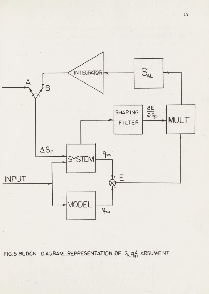
Further investigation proved this to be an analytic result, the consequence of rescaling a non-linear differential equation. One argument to demonstrate this is as follows: Considering Figure 5, if the input is f(t) and the switch in the adaptive loop is on B, there is

a waveform which is a function of time present at B. If this were to be recorded and then fed into the system through the switch which is now on A, but with a new input to the system of kf1(t), the output (q )

A

INPUT

SHAPING

MU

FILTER

ML

SP

_o

SYSTEM

MDE

-- MODEL

FIG. 5 BLOCK DIAG RAM REPRESENTATION OF S q? ARGUMENT

17

18 This is because the control system is now linear but with time-varying coefficients. The output of the multiplier will now be the original one

2 8E

multiplied by k since both E and are linear outputs. Now if

1 2

the adaptive loop sensitivity is changed from S AL to SAL

/k

1 A 1

input to the integrator will be the same as that forthe first system in-put and assuming the same initial conditions on the integrator, the output will also be identical. Hence, although the switch is at A the voltage at B is identical to that recorded on the first run and which we are now "tplaying back" into the system. Any two points in an electrical circuit at the same potential can be connected together without changing the operation of the circuit. Therefore the switch can be moved to B and the behavior of the system will not change.

The significance of this is to reduce the number of variables by one. If the behavior for a given input and initial parameter setting is known for all values of adaptive loop gain, the result of increasing the input by a factor of k is equivalent to using the original input, but increasing the adaptive loop g4in by k2 thereby causing (1) the

adaptive loop waveforms to be identical, and (2) the system output to be rescaled by exactly a factor of 1/k. This property of the system is

further demonstrated by the following chart:

Chart 1

Adaptive loop and system outputs are known for all values of SP int) and SAL with an input qin 1(t).

Then for qin (t) = k q in)

i2 . 1

Output of adaptive loop _ Output of adaptive loop with input #2 _{with input #1}

_I

Output of system with = Output of system input #2 = k x with input #1

19

3. 3 Linearity of Adaptation With Adaptive Loop Gain.

With a chosen input, flight condition, and initial parameter setting, the percent adaptation was found to vary linearly with adaptive loop gain up to 100% adaptation on the first step applied. This was an

experimental result, but was found to be true for all conditions tested. It is felt that this was because the parameter was not being changed

quickly enough to influence the transient solution; the second order effect being fed through the error and error derivative generators being negligible. It will be shown later that the lowest value of

adaptive loop gain giving 100% adaptation resulted in a minimum error.

3, 4 Instability Regions.

As SAL was increased beyond the 100% first step adaptation

value, for constant initial conditions and magnitude input, the solu-o tion would diverge but in two distinct ways. When the initial param-eter setting was below the optimum value, the control system was

2

very stable up to very high values of SAL 2 (See Appendix D,

Figure D-2.) and the system would then break into an oscillation with a real time frequency of about four cycles per second. This in-stability is illustrated in Appendix D, Figure D-5. No attempt was made to analyze the nature of this oscillation as it was felt that the

2

high value of SAL 2 did not represent realistic operation in a

physical system.

The second type of divergence would occur for initial param-eter settings above the optimum. At gains of about twice that re-quired for 100% first step adaptation, the adaptive loop would give the parameter a net change in the wrong direction. This is shown in Appendix D, Figure D-6... This was taken as a divergence, although

it will be shown later that this is not necessarily true if the system were allowed to continue to operate.

20

3& 5 Variation in SA 2With Initial Parameter Setting.

Probably the most significant of the various curves is that of 2

SAL 2nversus Sn for various percentages of adaptation after AL inp(init)

the first step. As an example of its use in describing the behavior for various step input magnitudes, see Figure 6a. Initially the parameter has a value of Sp(In t), and the input step has a

magni-tude that results in the SAq product shown at t1; the result of

the first step,since we are at a contour of 40%,adaptation,is to move the parameter . 4 of the way towards Sop The second input,

be.-cause it is larger in magnitude than the first, moves our position 2

vertically to the new SAL 2 line, which places the t2 position at

90% adaptation and we move . 9 of the way towards Sopt. The third input, larger still, moves us 1. 2 of the distance to Sopt. That is,

there is a 20% overshoot.

An illustration of what was meant by divergence not necessari-ly holding true if the system were allowed to continue operation is

shown in Figure 6b. With the input a series of plus and minus steps of constant magnitude, the same reasoning is followed as before. In Case A the input magnitude fixes our position on horizontal line a. It can be seen that after the application of the first step the adaptive loop changes the parameter in the wrong direction, but the application of the second step causes exactly 100% adaptation. In Case B with an

input such that our horizontal position is b, the reason for the rela-tive stability on the low side of Sopt is seen. The initial step causes

an overshoot of 100% but this repositions the parameter on the high side of optimum, where the succeeding steps cause the parameter to "walk" to the optimum.

4Oq

V

I

I

I

I

FIG.

6a

_{SIGNIFICANCE OF}

_SLcp

_vs

80%

$07.

SSO%

Si

22

200%

It,

ool

I.C

)7o

I

Spow~rr.

FIG 6b SIGNIFICANCE OF

-j

23

since the input is not necessarily a step nor is there always time be-tween inputs for the transients to die out, but it is felt that an

under-standing of this graph will give a better underunder-standing of what is happening in the adaptive loop.

For contours of first step adaptation this graph can be fairly easily realized up to contours of 100% for any particular adaptive configuration. This is due to the linear phenomenon mentioned be-fore: If the gain for 100% adaptation is known, all gains for lesser values of adaptation are directly proportional to the actual percentage adaptation. Thus the 100% contour fixes all those of lesser value. Caution must be exercised in determining the gain for 100% adapta-tion since this is sometimes ambiguous.

L 6 Gain Ambiguities for 100% Adaptation.

There were, in some cases, three values of adaptive loop gain that indicated the system was 100% adapted after the first step. In general, the first two values of adaptive loop gain were in agreement as to the value of S pt(See Figure 7b, the low and medium gain curves.), but the third which was always for the largest gain would indicate the parameter value had already been optimized when it was obvious that it had not. That is to say, that for the third case no net change was made in the parameter for either step. The apparent rea-son for this behavior was that the initial over-correction due to high gain was feeding into the transient solution with just the proper

amount of lag to cause a second equal and opposite correction, re-turning the parameter to its initial value. This is shown in Figure

7b, the high gain curve. The errors for the three values of S are AL shown in Figure Ua. It should be noted that the lowest gain results in the smallest error of the three.

Although in this study only one parameter was allowed to 2 adapt at a time, based on the work of Osburn, Whitaker, and Kezer,

HIGHEST

MMID

S4

LOWEST S0,1!

4

a.

ERROR

LOW

MID

S

-- HIGH

V.

I '\

AL

'

"I

ACf-b, PARAMETER CHANGE

FIG. 7 RESPONSES AT POINTS OF AMBIGUI TY

24

-30*

-0.465

111

I

I

I

/

\

/

TIM

I-TIME

i

TIME

25

it is felt that two or more parameters varying would probably im-prove the operation of the system.

Another interesting experimental result was found when 2

SAL 2nversus S was plotted on log-log paper. For points close to S optthe slope was very close to two to one, exhibiting a square

law variation. (See Appendix D, Figure D-4.) No useful result of this could be found other than a feeling for the variation of optimum gain with initial parameter setting. Possibly SAL could be made to

vary with Sp to improve the adaptability for a given input and initial

parameter setting.

3. 7 Variations in Adaptive Loop Sensitivity With Flight Condition. An attempt was made to correlate the adaptive loop sensiti-vity required for 100% adaptation with the control system open loop sensitivity, as well as with the optimum value of the adjustable

parameter. Experimental results indicated that each flight condition yielded a set of adaptive loop performance characteristics similar to those shown in detail for the supersonic cruise condition. However, the optimum adaptive loop gain curves did not coincide. In one case,

instability occurred at a lower gain than that required for 100% adap-tation for other flight conditions at the same initial parameter setting.

This would indicate that the adaptive loop sensitivity would have to be selected for the most critical flight conditions, and inferior perform-ance accepted for other conditions.

In one attempt to find some sort of functional relationship be-tween the adaptive loop gain, the adjustable parameter setting, and the flight condition, it was found that by making the adaptive loop

sen-sitivity a linear function of the adjustable parameter, plus a constant minimum value, reasonable performance could be attained at all flight conditions and initial parameter settings. This indicates the possibil-ity of mechanizing the adaptive loop sensitivpossibil-ity with the adjustable

26

parameter.

The reasons for this variation in adaptive loop performance with flight condition were not found. Further investigation of the causes of this behavior and the effect on the system design is indicated.

3. 8 Performance of the Adaptive System Using Limiters.

It has been shown that the adaptive loop sensitivity required for optimum performance of the adaptive loop was dependent on sev-eral variables. In an attempt to reduce the wide range of adaptive loop sensitivities required for optimum performance under various flight conditions, initial parameter settings, and input magnitudes, the adaptive loop was modified by inserting limiters in the error and

error derivative channels. The configuration with the limiters in-serted was as shown in Appendix A, Figure A-2.

Use of the limiters was based on non-linear system theory, which shows that the output of a limiting element followed by a low pass filter is independent of the input magnitude to the non-linear element, if the input is larger than the limit level, at least to the first approximation. It has been shown that the error and error derivative are each proportional tothe magnitude of the system input quantity. Therefore, the use of the limiters should make it possible to extract only that magnitude of the input quantity necessary to achieve optimum adaptation.

The limiters were chosen based on the following reasoning. Significant adaptation could be expected only for inputs larger than some minimum magnitude of the input quantity. This magnitude was chosen arbitrarily as a five degree roll command, a value typical of a trimming maneuver. The input limit level was chosen so that no clipping occurred for the error or error derivative at this input. The adaptive loop gain was then selected so that the amount of overcorrec-tion obtained for initial parameter settings below the optimum setting

2

were equal to the undercorrection obtained for initial settings an equal increment above optimum, for median expected input, chosen arbit-rarily as a 300 roll command. The median value was chosen as the point at which the compromise was to be made, since this would allow the performance for the large input quantities to remain within the stability limits while allowing near-optimum performance for the most used commands.

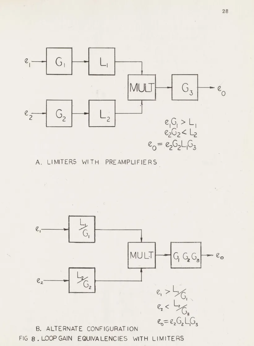
Since "loop gain" in a circuit containing non-linear elements is not clearly defined, the use of the term here may be clarified by referring to Figure 8. It may be noted that the circuits of Figure 8 are similar in configuration to the adaptive loop with limiters as shown in Appendix A, Figure A-2. In Figure 8a, arbitrary voltages, e and e2, are fed into amplifiers with gains GI and G2, then into

symmetrical limiters with unit gain and with limit levels L and L2 '

The outputs of the limiters are multiplied and amplified by a gain G₃" If it is assumed that limiter L 1 is in its limiting state, but that L2 is

in its linear region, then the output of the system is given by

e 0= L1e2G2G3 3-1)

In Figure 8b, the circuits are altered slightly by replacing the original amplifiers and limiters in the inputs by symmetrical unit gain limiters, each with limit level L/G. If the same conditions are

imposed on e ₁ and e₂ as in Figure 8a, it is apparent that again,

e0 = L1e2G2G3 (3-1)

The argument may be extended in an obvious manner for other valses 'of the input voltages.

28

MULT

_G

₃

---2

G2L

_eG

>

L,

1L2

e

_.e

_G

_L

G

A. LIMITERS WITH PREAMPLIFIERS

L

MU LT

G GG,

e

e

< L

B. ALTERNATE CONFIGURATION

29

The term Iadaptive loop gain' will then be defined as the loop output voltage with both limiters saturated, divided by the product of the saturation levels. In Figure 8, the adaptive loop gain is G3'

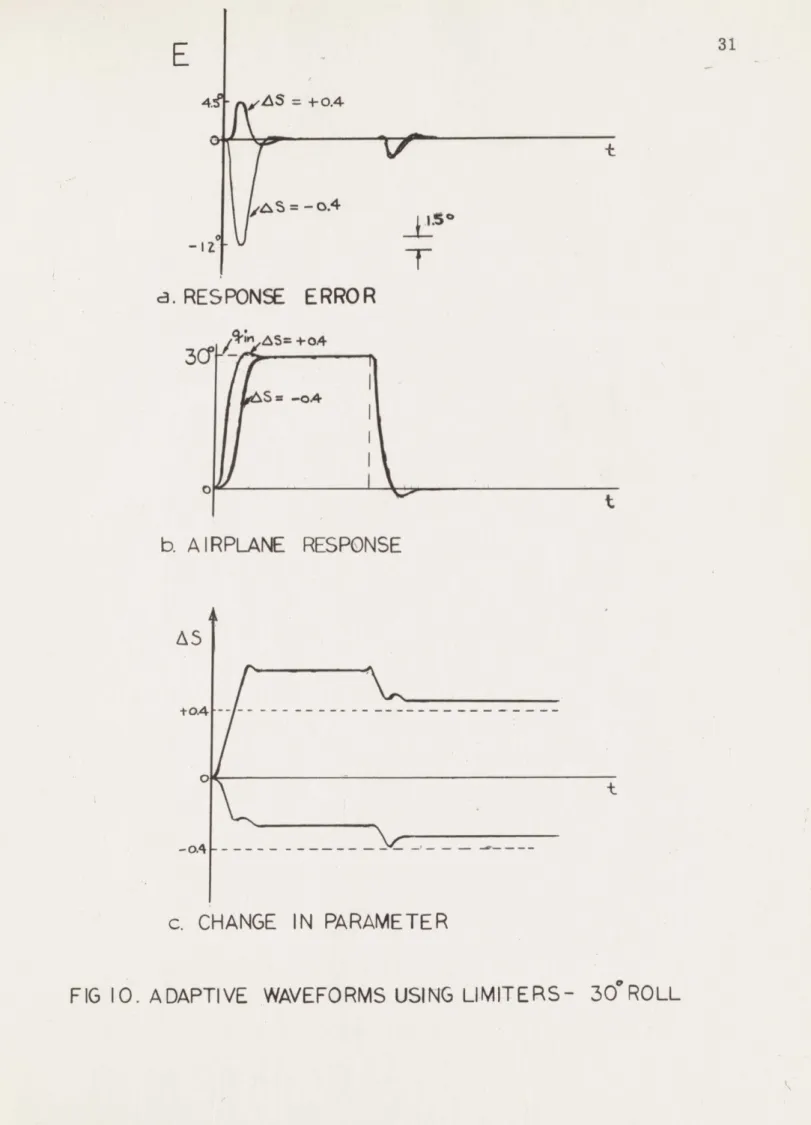
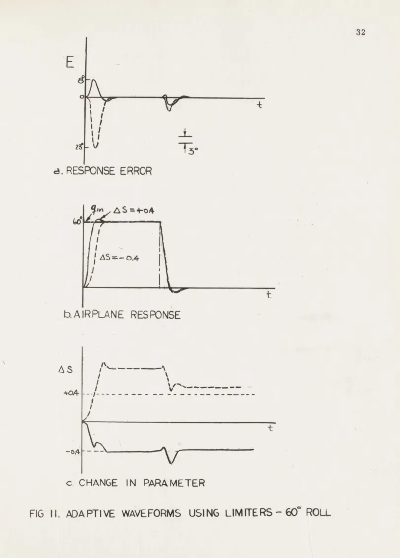
System responses were observed for several initial param-eter settings, each for three input step magnitudes. All observations were made without disturbing gain settings in the adaptive loop. Typ-ical results are shown in Figures 9, 10, and 11. In each figure, the aircraft response, the error quantity, and the parameter adjustment signals are shown for two initial parameter settings. The figures represent the responses for minimum, median and maximum expected input quantities, respectively.

It may be noted that in only one case was perfect adaptation achieved in one input step, namely, the 600 roll, Sp(init) = 0. 865. In

all cases a distinct improvement in system performance was observed, since in all cases the error was significantly reduced for the return step, and the difference in aircraft performance was indiscernable in all cases after the first correction, although sizable offsets of the adjustable parameter were made.

It was noted that with the limiter configuration of the adaptive loop, it was not possible to drive the adaptive loop into an instability

region with inputs as large as a 900 roll command. It was felt that this was a convincing argument for the use of such a system. With one setting of the adaptive loop sensitivity, the system was able to give reasonable performance for a very small input quantity, give good performance for a medium sized input, and yet remain stable for an input much larger than would be expected in any practical circum-stance. Under the system of instrumentation originally investigated, using the product of the error and error derivative directly, the value of adaptive loop sensitivity required to give 100% adaptation for a 600 roll command, would give only 7% adaptation for a five degree input, 25% adaptation for a 300 input. The figures show that the performance

E

Q9

o4

RESPONSE ERROR

I RPLANE RESPONSE

--7----/

I

/

t-c. CHANGE

IN PARAMETER

FIG.9. ADAPTIVE WAVEFORMS

=o.4

IA~

b. A

AS

5*ROLL

USING LIMI TERS

-I*l %! JS mam

---r tc 46wpah

E31

c.RESPONSE ERROR

b. AIRPLANE RESPONSE

AS

---c. CHANGE IN PARAMETER

32

E

RESPONSE ERROR

AS=-0.4

I

b.AIRPLANE RESPONSE

II

c. CHANGE IN PARAMETER

33

of the system was substantially better than this.

3. 9 Extension of Limiter Results to Other Configurations.

During the series of tests described, symmetrical limiters were used; I. e., the limit levels were the same for positive and negative signals. It may be noted that the adaptive loop output re-sponses were much greater for initial parameter settings below the optimum than for higher than optimum initial settings. This would indicate that a system employing an asymmetrical limiter would allow an equalization of the adaptation achievable on either side of the optimum setting. Such a limiter would be placed after the mul-tiplier, since it would be necessary to increase the effective adaptive loop gain for initial parameter settings higher than optimum and de-crease the effective gain for settings lower than optimum. Clearly, this could be done only for the weighted error, since both the error and the error derivative depend on the sign of the input, while the weighted error, which is a function of the input quantity squared, is independent of the sign of the input. Insufficient time was available to explore this possibility experimentally.

Another possible extension of the results of this study would be to simplify the mechanization by using the error derivative to actuate a relay, which would choose the proper sign of the error. This would eliminate the need for a multiplier in the adaptive loop. It is believed that it would be necessary to provide a finite null position on the relay, to prevent I hunting' when the parameter is near its optimum. This system would tend to give inferior performance for small inputs, i. e., those within the relay threshold level. This system was not evaluated experimentally.

CHAPTER 4

CONCLUSIONS

4. 1 Summary of Adaptive Loop Characteristics. 2

Identical SAL 2 products lead to an equivalency of operation

and identical adaptive loop outputs. This equivalency of operation is a general result, good for all types of inputs when multipliers and linear gains are used in the adaptive loop. Two related results of this are important:

1. The number of parameters to be investigated in a simu-lation program is reduced by one.

2 2. The instability boundaries are functions of the SAL 2

product,not of SAL alone.

2 The percentage adaptation is directly proportional to SALqin for all values of the product up to the lowest which achieves 100% first step adaptation. This gives a tremendous advantage since the

determination of the contour of 100% adaptation leaves only the opera-ting condition (Sopt) and Sp(init) to determine system behavior for

contours of lesser adaptation.

Instabilities with the multiplication and linear gain in the adaptive loop were of two types:

1. A relatively high frequency oscillation (4 cps) was found when SP(opt) >Sp(init), although this result may be a function of

2

system configuration. This occurred at such a high SALqin product 34

35

that it would not normally be a restricting factor in the design of adaptive loops.

2. The adaptive loop drove the parameter in the wrong direc-tion by the end of the transient soludirec-tion. Although it was shown that this may lead eventually to fully adapted solutions, it was considered

an instability and should be avoided in practice. The initial parameter settings were above S for this condition. The gains for this type

opt

of instability compared with those for 100% first step adaptation were found to have a ratio of about three with a minimum of about two.

Thus, insuring that SAL 2

I

<

instabilities of any nature. This further ties in with the linearity up to 100% adaptation, eliminating the requirement for plotting points above the 100% adaptation line. Thus, the plot of the single line de-termines all of the important characteristics for the flight condition.

With limiters in the adaptive loop no instabilities could be found within the range of useful operation of this system. Although

theS 2

the SALqn plot is, in a strict sense,,only for the original type of

adaptive loop configuration, the interpretation placed on this result is 2

that the lines of constant SAL 2 are warped by the limiter to more

closely follow the variation of 100% adaptation with Sp(init). In addi-2

tion, although increasing the input increases SAq2 the increase is

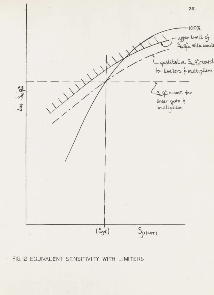
lessened above that value for which limiting starts, asymptotically approaching a limit for large values of input that is apparently below the instability point. This is illustrated in Figure 12.

2

The plot of SAL 2 versus S(init) for 100% first step

adap-tation showed a general second degree variation. This could be approximated analytically with either a first or second degree curve, suggesting that the adaptive loop gain could be instrumented as a function of parameter setting to achieve a constant amount of

36,

7

(52Kt)

WarlytLz

~y

FIG. 12 EQUIVALENT SENSITIVITY WITH LIMITERS

0

37

adaptation for a given input magnitude, regardlest of initial param-eter setting. The usefulness of this approach was limited by the variation in the curve with flight condition, I. e.., Sopte Although a

second order curve could still be used as an envelope of minimum SAL 21 , the various flight conditions gave rise to SAL 2

ALifor

A graphic and accurate outline of the system behavior is fairly easily obtained by simulation techniques. The model and approximate

2

aircraft are set up and five or six points of SAL 2 versus Sp init)

are run for 100% adaptation. The percentage adaptation is linear below this value, and the stability limit may be assumed to exceed these values by at least a factor of two. Repeating this for all four or five extremes in flight configuration completes the description of behavior for the whole spectrum of the control system' s environment.

The instrumentation as developed by Osburn shows an uncanny desire to achieve the desired result. In a case that was stumbled upon by accident, one parameter was being called upon to compensate for the accidental resetting of another and managed to do a very cred-itable job. It would seem, therefore, that the designer has the tools to obtain a very high quality of operation.

4. 2 Design Procedure.

Based upon the adaptive loop characteristics disclosed by this study two design procedures are outlined. The choice between the two procedures is based on the conditions under which the control system is to operate. It should be noted that the design of any

38

analogue simulation studies, since no convenient analytical design procedure has been found. It is felt that this is not a serious restric-tion, since any type of cofitrol system Operatim over a-wide range of

environmental conditions will very likely require simulation.

The design procedure suggested assumes that a system and model have been chosen, both of which are capable of performing their respective tasks. The selection of the appropriate model and a

control system configuration capable of performing the desired opera-tions is beyond the scope of this report and is adequately covered by earlier work. The procedure outlined below is specifically suited to

selection of an adaptive loop configuration and the required adaptive loop sensitivity.

1. Design Procedure using Multipliers and Linear Gains. In some cases, although the plant or process to be controlled is subjected to a variable environment, the input commands and desired response are constant, or encompass a very narrow

range. These conditions suggest the use of the adaptive system as illustrated in Appendix A, Figure A-1.

Before the adaptive loop sensitivity may be selected, estimates of the plant response characteristics for the various operating condi-tions must be made. These may be based on preliminary design

estimates, since the function of the adaptive loop is to render precise knowledge of the system performance unnecessary. Instead the

re-quirement is for an estimate of the range of the adjustable parameter. If the system is to be subjected to a range of input levels, the maxi-mum expected value of the input quantity must be known.

Armed with these system parameters, the designer should next obtain a contour or series of points in the S 2 S(init)

100% first step adaptation space for each operating condition. In finding this contour, cognizance should be taken of the folloWing facts:

39

sensitivity to at least 100% first step adaptation.

b. Equivalent results are obtained for identical 2SL2 products.

2

c. All instabilities are found at values of SAL 2 greater

than twice that required for 100% adaptation.

The adaptive loop sensitivity may then be selected. In general it will be advantageous to choose the adaptive loop gain to avoid all instability regions for the largest expected input.

Finally, the adaptive loop performance should be determined for the smallest input level for which significant adaptation is expected. If the performance for this input is not satisfactory, a more sophisti-cated adaptive loop configuration is indisophisti-cated.

2. Design Procedure using Two Limiters.

If the expected inputs have a wide range of values, a significant saving in simulation studies can be made. As with the system using linear gains, preliminary design estimates of the sys-tem characteristics in the various operating conditions are required as well as an estimate of the range of input magnitudes expected. This will allow the designer to find, either through simulation or through computation the approximate range of values for the adjustable parameter.

The limit level of each limiter (See Figure A-2 in Appendix A.) is set to pass its respective input function (error or error derivative) when the system is being excited by the minimum input for which sig-nificant adaptation is expected. The loop gain (defined in Chapter 3, Section 3. 8) is then chosen for good adaptation at a median input level. In general this setting will result in over correction when the initial parameter setting is on one side of the optimum value and undercor-recting when the initial setting is on the other. Finally the performance of the adaptive loop with the system excited by the maximum expected input should be surveyed for the various operating conditions, to

40

assure that the system is not unstable at any setting.

It is believed that these design procedures will result in a conservative design for the adaptive loop. First, during actual

operation of such a system, the parameter adjustment loop will track the optimum parameter setting in a smooth manner as the system moves from one set of operating conditions to the next (assuming no step discontinuities in environment or due to failures). Further, based on the work of Osburn, Whitaker and Kezer, the action of other adjustable parameters in a multiparameter system will have a favor-able effect on the system, both in response time and in improved stability.

41

APPENDIX A

+

+L

FIGA-I

ADAPTIVE ROLL FUGHTCONTROL SYSTEM BLOCK DIAGRAM

- -- - ADAPTIVE LOOP

MODEL

[.

-r

E

MODEL

MULT

CONTROL

SYSTEM

c, E

()S

MODEL

_L,

RATE

-

ULT

G

_SER0

--

_{MO DEL}

_L

*-- E2

FIGA2 ADAPTIVE LOOP WITH LIMITERS

APPENDIX B

AIRCRAFT CHARACTERISTICS

Summary of aircraft characteristics and the parameter values selected by the adaptive system.

Flight Conditions

No. Operating Regime

1 Supersonic cruise

2 Low speed and altitude

3 Landing

4 Acceleration to cruise altitude and speed 5 Subsonic climb Mach No. Aircraft Characteristics Altitude (Ft. ) 3. 5 75, 000 0.4 5,000 0.18 _sea level 2. 0 40, 000 0.9 10,000 sA[e,/de deg/sec/deg 9. 0 2. 2 1. 0 10. 0 4. 0 A (sec) Parameter values se-lected by adaptive sys. P 1P2 1 2 (eec) 3.00 0.465 1.00 1.00 .685 0.575 1. 80 2. 530 0.835 1.00 0.138 0.465 0.40 0,195 0 Model: wn x 1. 2 rad/sec; .,= 0. 70. Servo: rs= .1 _{S =} 44 Table 1.

45

APPENDIX C

Al

RCRAFT

MODEL

IWPUT To PA METEU.

2.!

FIG.

C-2

ERROR DERIVATIVE GENERATOR

+o --- 4 )PAL 1 mO i I TKE

r-44 Z-=Pio

CLAMP

MULT

--

(

--

AMP

aso-CLAMP

a.or

b

CLAMP

MULT

--

AMP

CLAMGP

________FIGURE

C-3 ADAPTIVE LOOP

APPENDIX

GRAPHICAL RESUL TS

49

D

2.53"

FUGHT COND.

Joo

Saw 0.465

FUGHT CON

010

FLIGHT COND.

S

0.132

FLIGHT

COND.

saw-O. 195

S.

2.53

11

%-PERCENT ADAPT

ON FIRST STEP

1.0

FIG. D-1

S

c

vs

,

FOR VARIOUS FLIGHT CONDITIONS

,

o.6e)

Io'

0*r

05

32

0-.95

FLIG4T COND.

, ,0.681

2.0

0.4E

51

100F

b. AS

=+0. 4

20

30

40

50

FIG D-2. PERCENT FIRST

100

STEP ADAPTATION

/ / /

I/I

/1

I/I

~'1

/1'

FIGD3.DEMONSTRATION OF Seqg EQUIVALENCY

52

60*

30'

INITIAL PARAMETER SETTING

06- _1.0

1.0

o.445 SOP*

LOG

pnI

FIG.D-4.

LOG -LOG PLOT

OF

53,

o.-2

54

To.6e

INPUT TO VARIABLE PARAMETER

EN

RES

PONSE

zi

ERROR

b. RESPONSE AND RESPONSE ERROR

EXAMPLE OF OSCILLATORY INSTABILITY

55

E

a.

RESPONSE

b

AIRPLANE

RESPONSE

CHANGE

PARAMETER

FIG. D-G. NON-OSCILLATORY

ERROR

0

\/

1-0\j

APPENDIX E

ANALYSIS OF THE ADAPTIVE SYSTEM

The basic assumption made is that the gain characteristic of the adaptive loop is as follows:

t

or

t

+.L+

go I )ijp

Fig. F-1. Gain Characteristic of Adaptive Loop

The value of A is assumed to be small, hence the operation to be analyzed is in the limited region where the output is a constant rate of change of adapted parameter, of magnitude L. Use is made

of the transform: Lt- L

3MP + S

Fig. F-2. Block Diagram

56