HAL Id: hal-01797619
https://hal.archives-ouvertes.fr/hal-01797619
Submitted on 22 Jun 2018HAL is a multi-disciplinary open access archive for the deposit and dissemination of sci-entific research documents, whether they are pub-lished or not. The documents may come from teaching and research institutions in France or abroad, or from public or private research centers.
L’archive ouverte pluridisciplinaire HAL, est destinée au dépôt et à la diffusion de documents scientifiques de niveau recherche, publiés ou non, émanant des établissements d’enseignement et de recherche français ou étrangers, des laboratoires publics ou privés.
Exchange across the sediment-water interface quantified
from porewater radon profiles
Peter Cook, Valenti Rodellas, Aladin Andrisoa, Thomas Stieglitz
To cite this version:
Peter Cook, Valenti Rodellas, Aladin Andrisoa, Thomas Stieglitz. Exchange across the sediment-water interface quantified from porewater radon profiles. Journal of Hydrology, Elsevier, 2018, 559, pp.873 - 883. �10.1016/j.jhydrol.2018.02.070�. �hal-01797619�
1 Exchange across the sediment-water interface quantified from porewater radon 1 profiles 2 3 4 5
Peter G. Cooka,b, Valentí Rodellasc, Aladin Andrisoac, Thomas C. Stieglitzc,d,
6 7 8 9 aNational Centre for Groundwater Research and Training (NCGRT), School of the 10 Environment, Flinders University, Adelaide SA 5001, Australia 11 bAix-Marseille Université, IMéRA, Marseille, F-13000, France 12 cCEREGE, Aix-Marseille Université, CNRS, IRD, Coll France, 13545 Aix-en-Provence, 13 France 14 dCentre for Tropical Water and Aquatic Ecosystem Research, James Cook 15 University, Townsville, Queensland 4811, Australia 16 17 Corresponding Author: Peter Cook ([email protected]) 18 19 20
2 HIGHLIGHTS: 21 • The radon profile method for estimating porewater exchange is reviewed 22 • A simple recirculation model is presented to aid in profile interpretation 23 • Uncertainties in the approach are discussed 24 25
3 ABSTRACT 26 27 Water recirculation through permeable sediments induced by wave action, tidal 28 pumping and currents enhances the exchange of solutes and fine particles between 29 sediments and overlying waters, and can be an important hydro-biogeochemical 30 process. In shallow water, most of the recirculation is likely to be driven by the 31
interaction of wave-driven oscillatory flows with bottom topography which can induce 32 pressure fluctuations at the sediment – water interface on very short timescales. 33 Tracer-based methods provide the most reliable means for characterizing this 34 short-timescale exchange. However, the commonly applied approaches only 35 provide a direct measure of the tracer flux. Estimating water fluxes requires 36 characterizing the tracer concentration in discharging porewater; this implies 37 collecting porewater samples at shallow depths (usually a few mm, depending on 38 the hydrodynamic dispersivity), which is very difficult with commonly used 39 techniques. In this study, we simulate observed vertical profiles of radon 40 concentration beneath shallow coastal lagoons using a simple water recirculation 41 model that allows us to estimate water exchange fluxes as a function of depth 42 below the sediment-water interface. Estimated water fluxes at the sediment water 43 interface at our site were 0.18 – 0.25 m/day, with fluxes decreasing exponentially 44 with depth. Uncertainty in dispersivity is the greatest source of error in exchange 45 flux, and results in an uncertainty of approximately a factor-of-five. 46 47 48 KEYWORDS: porewater exchange, recirculated seawater, benthic flux, lake, tracers, 49 radon 50
4 1. INTRODUCTION 51 Water recirculation through permeable sediments enhances the exchange of 52 solutes and fine particles between sediments and overlying waters. In particular, it 53 allows for a continuous supply of oxidants and fine particulate and dissolved 54 matter (e.g. dissolved nutrients, bacteria, viruses, phytoplankton) into sediment 55 porewaters, while enhancing the release of degradation products and organisms 56 into overlying waters (Huettel and Rusch, 2000; Huettel et al., 1996). As a 57 consequence, porewater exchange is considered a major contributor to the 58 biogeochemical cycling of surface sediments and overlying waters, particularly in 59 the coastal zone (Anschutz et al., 2009; Huettel et al., 2014, 1998; Jahnke et al., 60 2005). Porewater exchange increases in importance in highly-permeable sandy 61 sediments, which cover >40% of coastal and shelf areas worldwide (Riedl et al., 62 1972), where this advective transport of solutes can exceed fluxes driven by 63 molecular diffusion by several orders of magnitude (Huettel and Webster, 2001). 64 This advective exchange between porewaters and overlying waters is caused by 65 pressure gradients at the sediment-water interface, which might be forced by 66 several mechanisms spanning a range of spatial and temporal scales, including 67 wave and tidal pumping, interaction of bottom currents and seafloor topography, 68 density instabilities or pumping activities of benthic fauna (bio-irrigation, Huettel 69 et al., 2014; Santos et al., 2012). For instance, the passage of waves can produce 70 oscillatory flows that interact with bottom topography (e.g. ripples), producing 71 local increases of pressure that drive fluid exchange across the sediment-water 72 interface. In addition, the passage of wave crests and troughs creates pressure 73
5 gradients over the seafloor that also enhance porewater exchange (Riedl et al., 74 1972; Rutgers van der Loeff, 1981; Webster, 2003). 75 Despite the importance of porewater exchange in coastal biogeochemical cycles, it 76 is still not easy to quantify the advective flux of water and solutes in permeable 77 sediments (Boudreau et al., 2001; Rocha, 2008). Common methods to estimate the 78 rate of porewater exchange across the sediment-water interface in permeable 79 sediments include (1) deploying automated seepage meters to monitor the 80 porewater flow into overlying waters (e.g. Jahnke et al., 2000; Cable et al., 2006), 81 (2) constructing mass balances in overlying waters for a tracer supplied by 82 porewater inputs (e.g. Stieglitz et al., 2013; Rodellas et al., 2017), (3) injecting 83 artificial tracers or dye into or above the sediments to trace fluid advection across 84 the sediment-water interface (e.g. Reimers et al., 2004; Precht and Huettel, 2004), 85 and (4) modeling the depth profiles of temperature, electrical conductivity or 86 dissolved species in sediments to evaluate the sediment-water exchange rates (e.g. 87 Cable and Martin, 2008; Savidge et al., 2016). Among these dissolved compounds, 88
short-lived, naturally-occurring radionuclides (e.g. 224Ra and 222Rn) have been
89 widely used, mainly because their half-lives are well suited to the common 90 timescales of these porewater exchange processes (e.g. Colbert and Hammond, 91 2008; Cable and Martin, 2008; Cai et al., 2014). Radium-224 (half-life = 3.6 d) is 92 produced by radioactive decay of 228Th, but partitions to aquifer solids which 93 reduces the sensitivity of dissolved 224Ra activities to porewater exchange fluxes. 94 As a noble gas, radon (222Rn; half-life = 3.8 d) is an excellent tracer of porewater 95 exchange because it is not affected by chemical and biological processes occurring 96 within sediments. In this study, we review the application of radon porewater 97
6 profiles in sediments to estimate the porewater exchange across the sediment-98 water interface driven by pressure fluctuations on short time-scales, such as those 99 produced by wave action. We simulate observed radon profiles using a numerical 100 model of water recirculation that allows us to estimate porewater exchange rates 101 as a function of depth below the sediment-water interface, and to explore 102 sensitivity of estimated fluxes to model parameters. An alternative simpler 103 approach is also presented, where water fluxes are estimated based on changes in 104 the observed radon concentration gradient with depth. 105 106 2. THEORY 107 Radon-222 is a natural environmental tracer that has been used for quantifying 108 groundwater inflows to streams and estuaries (e.g. (Cook et al., 2006; Genereux et 109 al., 1993)) and the ocean (e.g. (Cable et al., 1996)) for almost three decades. Radon 110 is produced in the sediments by the radioactive decay of 226Ra, which is part of the 111 238U decay chain and it is found in the sediment solids and in porewater. After 112 porewater containing radon discharges to surface water bodies, radon activities in 113 the surface water decrease due to gaseous exchange with the atmosphere and 114 radioactive decay. Radon concentrations in surface water are therefore always 115 much lower than concentrations within porewaters. When surface water 116 infiltrates, its dissolved radon concentration will increase, according to 117 !! !! = γ − λc (1) 118
7 where c is the radon concentration, γ is the production rate of dissolved radon, λ is 119 the radon radioactive decay coefficient (0.1818 d-1), and t is time. After a residence 120 time of a few weeks the concentration will reach secular equilibrium, in which the 121 rate of production is exactly balanced by the rate of radioactive decay. The 122 concentration at secular equilibrium is equal to γ/λ. If the radon production rate 123 within the sediments is constant, then the radon concentration in porewater 124 beneath the seafloor will increase with depth, up to a depth where secular 125 equilibrium is reached. The depletion of radon at shallow depths may therefore be 126 used to derive the exchange between porewater and overlying waters. 127 128 2.1. Radon deficit model 129 The most commonly applied approach to estimate the flux of radon across the 130 sediment-water interface is based on the deficit of porewater radon relative to 131 radon concentrations at secular equilibrium, i.e. the radon concentration that 132 would occur without solute exchange (e.g. Martin et al., 2007; Cable and Martin, 133 2008). This deficit must be equal to the total net flux of radon into overlying 134 waters. More generally, and assuming 1D flow, the net radon flux at depth z’ can be 135 written as: 136 𝐽!" = !!! 𝛾 − 𝜆𝑐 𝜃𝑑𝑧 (2) 137 where θ is sediment porosity and c is the radon concentration at each depth z. 138 Integrating from z’=0 to ∞ gives the net radon flux across the sediment-water 139 interface. 140
8 Aside from the sediment porosity and the radon concentrations at the different 141 depths, this approach requires knowledge of the production rate in sediments (γ), 142 which can either be calculated from slurry-equilibration experiments (Colbert and 143 Hammond, 2008) or derived from deep porewater radon concentrations, which 144 are assumed to be unaffected by porewater exchange (Cable and Martin, 2008). 145 146 2.2. Advection cycling model 147 Exchange of solutes between rivers and lakes and underlying porewaters has 148 frequently been simulated using mass balance models that represent the 149 porewater zone as a perfectly mixed reservoir of constant depth (Bencala, 1983; 150 Cook et al., 2006; Gooseff et al., 2003; Stieglitz et al., 2013). Multiple reservoirs 151 sometimes have been used, although such reservoirs usually operate in parallel so 152 that each reservoir is directly connected to the surface water (Choi et al., 2000). In 153 most cases, the focus of these studies has been on reproducing exchange fluxes 154 rather than porewater concentrations, although Lamontagne and Cook (2007) 155 used a single reservoir model to relate water fluxes to radon concentrations within 156 porewater of a river hyporheic zone that was assumed to be perfectly mixed. 157 As the objective of the present study is to interpret vertical radon profiles rather 158 than mean porewater concentrations, we consider a series of vertically-stacked 159 reservoirs rather than a single reservoir. This type of model, sometimes referred to 160 as a compartmental mixing model, has been widely applied in soil water and 161 groundwater transport simulations (Adar et al., 1988; Harrington et al., 1999; Kirk 162 and Campana, 1990), but not previously in the context of porewater exchange. 163
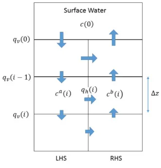
9 Water and solutes are assumed to be perfectly mixed within each cell, and only 164 advective fluxes between the cells are considered. Thus hydrodynamic dispersion 165 is simulated implicitly through mixing within the cells rather than explicitly 166 included in the governing equations. Compartmental mixing cell models have been 167 shown to produce similar results to advective-dispersive models provided that 168 advection is the dominant transport process and that the size of the mixing cell is 169 appropriately chosen (Xu et al., 2007). 170 The model presented here represents a two-dimensional recirculation cell, in 171 which flow reverses periodically. This type of flow system might be produced by 172 the passage of waves across the water surface, with surface water moving into the 173 sediments beneath the wave peaks (high pressure), and exiting beneath the wave 174 troughs (low pressure). We assume that the vertical scale of the recirculation cell 175 is much greater than the horizontal scale, so that horizontal travel times are 176 negligible (this is discussed further below). The two-dimensional model thus 177 collapses into two one-dimensional profiles that exchange water and solutes. The 178 fully saturated porewater zone is discretized into a number of layers (cells), each 179 of which is assumed to be perfectly mixed. Each cell is assumed to continually 180 exchange water with the cells immediately above and below it (the uppermost cell 181 representing the surface water), and also to exchange water with the cell at the 182 equivalent depth in the adjacent profile (Figure 1). The downward flow in one 183 profile is thus balanced by the upward flow in the second profile, and the change in 184 vertical water flux with depth determines the exchange flux between the two 185 profiles. For each profile, we solve 186 ! !" !" = − ! !" 𝑞!𝑐 + 𝛾𝜃 − 𝜆𝜃𝑐 − 𝑆 (3) 187
10 where 𝑞! is vertical water flux (which is a function of depth), and S is a mass flux 188 term that allows for flow between the upwelling and downwelling profiles. 𝑞! is 189 defined so that downward fluxes are positive and upward fluxes are negative. 190 Dispersion is not explicitly simulated, but it is implicitly simulated based on the 191 size of the mixing cells. The relationship between cell size (Δz) and implicit 192 dispersivity (α) is given by (Kirchner, 1998; Shanahan and Harleman, 1984): 193 𝛼 =∆!! (4) 194 The water flux decreases with depth in the downwelling profile, so that for the first 195 phase of the recirculation cycle, water moves downward on the left hand side and 196 upwards on the right hand side, as shown in Figure 1. Horizontal flows occur from 197 left to right, and are given by 198 𝑞! 𝑖 = 𝑞! 𝑖 − 1 − 𝑞! 𝑖 (5) 199
where 𝑞!(𝑖) is the horizontal water flux at the depth represented by cell i, qv(i-1) is
200
the downward water flux into cell i from the overlying cell and qv(i) is the vertical
201
water flux from cell i into the underlying cell. Note that both qv and qh are
202 volumetric fluxes per square area of the sediment surface, and so qh is not a Darcy 203 velocity in the traditional sense. Note also that the term S in Equation 3 can be 204 obtained by multiplying qh(i) by the concentration in cell i of the downwelling 205 profile. S will therefore be positive for downwelling profiles (-S is negative, 206 representing a mass loss) and negative for upwelling profiles (-S is positive, 207 representing a mass gain). 208 The solute mass balance equations are: 209
11 ∆𝑐! 𝑖 = ∆𝑡 !!! !!! ! !! !!! !!! ! ∆! + 𝛾 − 𝜆𝑐! 𝑖 (6) 210 211 ∆𝑐! 𝑖 = ∆𝑡 !!!! ! ! !!!!! !!!! ∆! + !!!! !!!!!!! ! !!! !!! ! ∆! + 𝛾 − 𝜆𝑐 ! 𝑖 (7) 212
where c is concentration, Δc is change in concentration, 𝑞! and 𝑞! are the vertical
213 and horizontal water fluxes, Δz is the vertical cell dimension, Δt is the temporal 214 discretization and the superscripts 𝑎 and 𝑏 denote the fluxes and concentrations in 215 the downward-flow and upward-flow cells respectively (symmetry of the 216 recirculation cell requires that 𝑞!! = −𝑞 !!). 217 After a period of time (tr/2), the flow reverses, and so the directions of all arrows 218 shown in Figure 1 reverse. The calculations are then repeated, with superscripts 𝑎 219 and 𝑏 switched in Equations 6 and 7. This cycle is then repeated. Because the 220 direction of flux changes during the recirculation cycle, the mean upward and 221 downward water flux at each depth across a complete recirculation cycle (𝑞!) is 222 calculated by dividing 𝑞! by two (i.e. 𝑞! = 2𝑞!). 223 The upper boundary condition is constant concentration (c=c0). The lower 224 boundary is the concentration of radon in equilibrium with the rate of production 225 (c=γ/λ), although in practice the lower boundary is set to be sufficiently deep so 226 that it does not affect simulation results. The key parameters in the model are the 227 concentration in the overlying surface water (c0), the sediment characteristics (θ, 228 γ), and the characteristics of the recirculation, which include the time for a 229
completed cycle (tr), and the velocity profile qv(i).
12 It should be noted that as the period of the recirculation (tr) becomes small, radon 231 concentrations derived from the oscillating flow model are equivalent to those 232 observed in a simple 1D steady state model with flow occurring simultaneously in 233 both directions. This is given by 234 !!!!! ! ! !!! !! ! ∆! − !! ! ! ! ! !! !!! ∆! + 𝛾 − 𝜆𝑐 = 0 (8) 235 236 2.3. Dispersion model 237 For small recirculation times (tr), the solute profiles in a reversing flow field can 238 also be expressed in terms of an enhanced dispersion coefficient, rather than by 239 directly simulating advection (Qian et al., 2009). The flux of radon at any depth can 240 be expressed 241 𝐽!" = 𝐷!𝜃!"!" (9) 242
where JRn is the radon flux and De is the enhanced dispersion coefficient (m2 d-1).
243 Qian et al. (2009) developed a two-dimensional hydraulic model to examine the 244 effect of wave action on porewater solute profiles, and showed that the value of the 245 enhanced dispersion coefficient decreased exponentially with depth, and could be 246 approximated by 247 𝐷!(𝑧) =!!"#!" 𝑒𝑥𝑝 !!.!"!! (10) 248 where K is the sediment hydraulic conductivity, a is the half-wave amplitude and L 249 is the wavelength (m). 250
13 251 3. METHODS 252 3.1. Radon sampling: study site, sampling and analyses 253 Porewater profiles for radon analysis were collected at La Palme lagoon, located 254 on the western French Mediterranean coastline. La Palme is a small (5 km2 surface 255 area), shallow lagoon, with mean and maximum water depths of 0.6 and 1.5 m 256 respectively. It is connected with the Mediterranean Sea through a small opening 257 in the coastal sand spit and it receives continuous fresh groundwater inputs 258 mainly from a regional karst aquifer (Stieglitz et al., 2013). The internal mixing of 259 the lagoon and its exchange with coastal waters is driven primarily by the strong 260 north-westerly winds characteristic of the region (regularly exceeding 10 m/s). 261 Tidal forcing plays a minor role on the hydrodynamic functioning of this lagoon 262 (tidal variations in the Mediterranean Sea are usually less than 0.4 m and exchange 263 between the lagoon and the sea is highly restricted). Most of the lagoon is covered 264 by coarse-grained highly-permeable sediments. A recent study conducted by 265 Stieglitz et al. (2013) revealed that wind-driven horizontal pressure gradients at 266 the sediment-water interface produce the recirculation of large amounts of lagoon 267 water through surface sediments. Indeed, they estimated that the equivalent of the 268 volume of the entire lagoon recirculates through the sediments every 25 days. La 269 Palme is thus an ideal site to evaluate the exchange of porewater across the 270 sediment-water interface by using radon porewater profiles. 271 Porewater samples for radon analysis were collected at 2 different locations (Pz1 272
at 42.9741°S, 3.0163°E and Pz2 at 42.9391°S, 3.0248°E) using a drive point 273
14 piezometer. At each location, samples were collected at depths of 0.05 (only Pz1), 274 0.10, 0.15, 0.20, 0.30, 0.50, 0.80 and 1.30 (only Pz2) m below the sediment – water 275 interface. 10-mL porewater samples were collected using a gas-tight syringe 276 coupled to the piezometer tubing (minimizing water-air contact) and transferred 277 to 20-mL vials prefilled with a 10-mL high-efficiency mineral oil scintillation 278 cocktail (Cable and Martin, 2008). Concentrations of radon were analyzed by liquid 279 scintillation counting on a Quantulus 1220 with alpha-beta discrimination 280 counting (background of 0.2-0.4 cpm; efficiency of 1.6-2.2, depending on the 281 quenching factor of the sample). Surface water samples (2 L) were collected using 282 a small submersible pump to minimize the gas loss and analyzed using the radon-283 in-air monitor RAD7 coupled to an extraction system. Samples were decay-284 corrected to the time of collection. 285 286 3.2. Model 287 The advective compartmental mixing cell model was programmed into Fortran 95. 288 We used a cell size of Δz = 0.01 m, which is equivalent to an implicit dispersivity of 289 α = 0.005 m. The latter is consistent with a flow length of approximately 0.5 m 290 (Gelhar et al., 1992). (This is the approximate depth of radon depletion apparent in 291 the measured profiles, and hence also the apparent depth of recirculation.) 292 Temporal discretization was 10-7 days (0.0086 seconds), but identical results were 293 obtained using smaller values. The model was run for at least 20 days, so that 294 radon concentrations reach dynamic equilibrium and are unaffected by initial 295
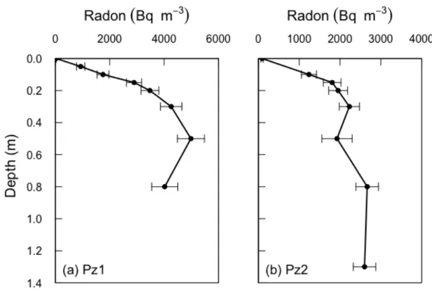
15 conditions. Sediment porosity and radon production rate were both assumed to be 296 constant (i.e., do not vary with depth). 297 298 4. RESULTS 299 The two porewater profiles Pz1 and Pz2 showed radon concentrations increasing 300 rapidly with depth up to around 30 - 50 cm depth. Radon concentrations below 301 these depths were relatively constant, with maximum concentrations of 302
approximately 5000 Bq m-3 and 2500 Bq m-3 for Pz1 and Pz2 respectively, which
303 likely reflect concentrations reaching secular equilibrium. The lower value 304 observed at 0.8 m for PZ1 is likely due to analytical or sampling uncertainty or may 305 reflect a spatial variation in the radon production rate. The difference between the 306 measured radon concentrations at shallow depth and these equilibrium 307 concentrations sustained by the production rate indicates that there is a significant 308 exchange of radon between porewaters and overlying waters. 309 310 4.1. Deficit model 311 The radon production rates for the two sites are approximately 900 and 450 Bq m3 312 d-1 for Pz1 and Pz2, respectively, as derived from the maximum concentrations 313 measured at each site (assuming constant production rates over depth). By 314 applying equation 2 and using a porosity (θ) of 0.4, we estimated a total net flux of 315 radon into overlying waters of 58 and 38 Bq m-2 d-1 for Pz1 and Pz2, respectively. 316
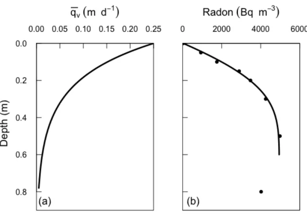
16 The radon flux estimated here refers to the total net loss of radon from sediments 317 into surface waters and thus includes also the flux of radon supplied by molecular 318 diffusion. The net advective-dispersive flux of radon from sediments can be 319 calculated as the difference between the estimated total flux and the diffusive flux, 320 which can be approximated using Fick’s First Law and radon diffusion coefficients 321 corrected for both temperature and tortuosity (~1 × 10⁻⁴ m2 d-1; (Boudreau, 1997; 322 Li and Gregory, 1974)). By using the radon gradients over depth measured in the 323 shallowest porewaters (above 20 cm), the diffusive flux is on the order of 10-1 Bq 324 m-2 d-1, which is 2 orders of magnitude lower than the total radon flux. Therefore, 325 radon diffusive fluxes in the studied profiles can be neglected and the total 222Rn 326 flux can be attributed to advective-dispersive fluxes. 327 328 4.2. Advection cycling model 329 Observed radon profiles were simulated using constant surface water 330 concentrations of 30 (Pz1) and 90 (Pz2) Bq m-3, and 𝑞 ! 𝑧 and 𝑡! were varied in a 331 trial-and-error fashion, until good fits with observed profiles were obtained. It was 332 found that best-fits to radon profiles were produced with water fluxes that 333 decreased exponentially with depth, and so this was adopted in all simulations. 334 The simulated radon profile for Pz1 is shown in Figure 3, and closely matches the 335 observed profile to a depth of 0.5 m. This simulation uses a recirculation time of 336 tr/2 = 10-5 days (0.864 seconds), although identical profiles are produced for 337 recirculation times on the order of <10-2 days. For longer times, different 338 upwelling and downwelling profiles are obtained (Figure 4). In this case, the 339
17 profile that has just completed its downwelling phase (orange line in Figure 4) has 340 much lower concentrations than the upwelling profile (blue line). This essentially 341 represents differences that would be observed depending on the sampling time in 342 relation to the phase of the cycling. 343 The mean upwelling or downwelling water flux across the sediment – water 344 interface in Pz1 is 𝑞! 0 = 0.25 m d-1 (3 × 10⁻⁶ m s-1). The radon flux from the 345
surface into the underlying cell is 𝑞! 0 𝑐 0 , which is equal to 7.5 Bq m-2 d-1. The
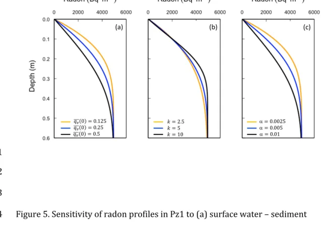
346 radon concentration in this second cell (immediately below the surface water 347 layer) is 240 Bq m-3, and so there is also an upward radon flux into the surface 348 water of 𝑞! 0 𝑐 1 = 61 Bq m-2 d-1. The net radon flux into the surface water is 349 therefore 𝑞! 0 𝑐 1 − 𝑐 0 = 54 Bq m-2 d-1. This is essentially the same as the 350 radon flux for Pz1 calculated from Equation 2 (58 Bq m-2 d-1). 351 Figure 5 depicts the sensitivity of the radon profiles to variations in surface water– 352 sediment exchange flux (𝑞! 0 ), attenuation of water flux with depth (k), and 353 implicit dispersivity. The latter is investigated by varying the cell dimensions in the 354 model. The simulations show, that if dispersivity is fixed, then if sampled with 355 sufficient resolution, the radon profiles allow unique determination of 𝑞! 0 and k, 356 as these parameters affect the profiles in different ways. In particular, varying k 357 only affects the deeper parts of the profile. However, dispersivity and velocity 358 affect radon profiles similarly, indicating model non-uniqueness. Assuming a value 359 for dispersivity is therefore essential for estimating the water flux. In our case, 360 fitting the radon profiles with dispersivities of 0.0025 and 0.01 m2 d-1 (cell sizes of 361 0.005 and 0.02 m, respectively) would have resulted in mean surface water fluxes 362 of 0.5 and 0.125 m d-1 m respectively. 363
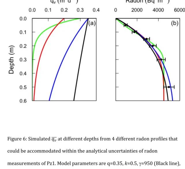
18 Additionally, the uncertainties associated with radon analytical measurements 364 allow for accommodating different radon profiles (for a fixed dispersivity), and 365 thus yield different simulated k and 𝑞! values (Figure 6). Thus, within the error 366 bars of the radon measurements, surface water fluxes of 𝑞! 0 = 0.2 – 0.35 m d-1 367 and flux attenuation rates of k = 0.5 – 15 m-1 are possible. However, the lowest 368 values of k are only possible if the two shallow radon values (< 0.15 m depth) are 369 towards the upper limit of the analytical uncertainty range, and the four deeper 370 values (0.15 – 0.5 m) are towards the lower limit. The reverse applies for the 371 higher values of k. This is extremely unlikely to be the case (probability of 2-6; or 372 less than 2%). Thus, the true uncertainty in k is much less than this, and probably 373 closer to 2.0 < k < 10 m-1. Values of k are most sensitive to radon concentrations at 374 0.2 – 0.4 m depth (Figure 5), and increasing the precision of these measurements 375 would significantly improve the accuracy of the flux attenuation rate estimate. 376 Radon concentrations in profile Pz2 are reproduced using a production rate of γ = 377 450 Bq m-3 d-1, and surface flux 𝑞! 0 = 0.18, but with other parameters identical 378 (θ = 0.4; 𝑡!/2= 10-5 d (0.86 s); with k = 5 m-1). 379 380 4.3. Dispersion Model 381 It is also possible to represent the observed radon data in terms of enhanced 382 dispersion coefficients rather than explicitly considering advective fluxes. By 383 equating Equations 2 and 9, we obtain 384 𝐷!𝜃!" !!!!!" = !!! γ − 𝜆𝑐 𝜃𝑑𝑧 (11) 385
19 The dispersivity profile can therefore be obtained by approximating !"!" using the 386 observed changes in radon concentration between sampling depths and solving 387 Equation 11. 388 The profile of enhanced dispersion coefficient calculated for profile Pz1 in this way 389 is depicted in Figure 7a. The dispersion coefficient is related to the flux by 390 𝐷! = 𝑣 𝛼, where ν is the water velocity. As dispersion will occur under both 391 upward and downward flow, it is therefore related to the recirculation flux 392 according to 393 𝐷! =!!!! = !!!!! (12) 394 where 𝑞! is the upward or downward flux that occurs during respective upwelling 395 and downwelling phases, and 𝑞! is the mean upward or downward flux averaged 396 across the two phases. Thus we can calculate the average flux 𝑞! by rearranging 397 equation 12. This is shown in Figure 7b, where it is also compared with the flux 398 profile obtained from the advection cycling model. The surface flux calculated 399 using Equations 11 and 12 is 0.31 m d-1, which is similar to that calculated from the 400 mixing cell model (0.25 m d-1). 401 402
20 5. DISCUSSION 403 5.1. Model sensitivity 404 The results from both the advection cycling and the dispersion model are a 405 function of the selected longitudinal dispersivity (expressed as cell size for the 406 advection cycling model). Changing the selected dispersivity will result in 407 proportional changes on the estimated water fluxes. Since dispersivity is a scale 408 dependent parameter, longitudinal dispersivity (α) has been often related to the 409 length of the flow path at the field scale (Gelhar et al., 1992; Neuman, 1990). 410 Assuming a flow path length of 0.5 m, we would obtain an approximate 411 dispersivity of 0.005 m, which is the value used in this study. The estimated 412 dispersivity would largely depend on the length scale selected, which may be 413 difficult to define when dealing with porewater fluxes. As an alternative 414 approximation, Qian et al. (2008) suggested that pore-scale dispersivities in a 415 sediment bed can be approximated by the average particle size. Since the sediment 416 of the study site are mainly composed by coarse-grained particles, the mean 417 particle size is likely ranging from half to a few millimeters, and the expected range 418 of α would therefore be on the order of 0.001 m. This gives a factor-of-five 419 uncertainty in α, and hence also in water flux. 420 Aside from longitudinal dispersivity, which is the single most important control on 421 model results, the advection cycling model is also sensitive to other input 422 parameters. Although exchange flux (𝑞!) is proportional to porosity (θ), this 423 parameter is relatively easy to estimate in unconsolidated sediments, and it is not 424 expected to vary in a wide range. The radon production rate (γ) is constrained by 425 the radon concentrations measured in deep porewaters, and so it is important for 426
21 samples to be collected from sufficient depth. In our example, γ was assumed to be 427 constant with depth, although variations in θ and γ with depth can be introduced to 428 the model if they are expected to occur. In this case, γ would need to be derived 429 from equilibration experiments, and previous studies have shown that these 430 measurements can have significant uncertainties (Key et al., 1979; Berelson et al., 431 1982). Model-derived water fluxes in the uppermost layers of the sediment are 432 relatively insensitive to the selected production rate (γ), but γ exerts an important 433 control on the water fluxes simulated for deeper layers, where radon 434 concentrations approach secular equilibrium. Accurate estimation of water fluxes 435 at depth, and the rate (and functional form) of flux attenuation, is also highly 436 sensitive to the analytical precision of radon measurements. We assumed that 𝑞! 437 decreased exponentially with depth, as this is commonly assumed (e.g. Qian et al., 438 2009; Fram et al., 2014; Wilson et al., 2016) and because the exponential decrease 439 produced the best fit to the data. Finally, the model is not very sensitive to 440 variations in the time for each phase for the cycle when tr is on the order of <10-2 441 days. For a given value of dispersivity, the uncertainty in all these input 442 parameters and analytical precision result in an uncertainty in the water flux 443 across the sediment – water interface (𝑞! 0 ) of approximately a factor-of-two. 444 Thus, as previously discussed, uncertainty in dispersivity dominates the 445 uncertainty in surface water flux. 446 A limitation of the model is that it neglects horizontal travel times between 447 downwelling and upwelling profiles. This may be reasonable for small-scale 448 recirculation driven by wave action, as at any time upwelling and downwelling 449 zones are likely to be separated by only a few centimetres. The assumption is less 450
22 likely to be valid for recirculation systems driven by processes operating over 451 longer timescales, such as seiches or tides. For these, porewater concentrations 452 (such as those shown in Figure 4) are likely to be underestimated, particularly for 453 upwelling profiles. 454 455 5.2. Quantification of water exchange across the sediment-water 456 interface 457 A number of previous studies have estimated net radon fluxes across the 458 sediment–water interface by integrating the radon deficit in sediment porewater 459 (Equation 2) (e.g. Cable and Martin, 2008; Martin et al., 2007). However, it is not 460 straightforward to calculate the water flow from this data. The common approach 461 to convert this radon flux into specific porewater discharge is by dividing the mass 462 flux by the radon concentration in the shallowest porewater sample (Cable and 463 Martin, 2008; Martin et al., 2007). Given that it is extremely difficult to collect 464 porewater samples for radon analysis in the top centimeters of the sediment, the 465 nearest-surface porewater samples are commonly collected at 0.05-0.1 m depth. In 466 the case of the profiles collected in La Palme lagoon, the radon concentration in the 467 uppermost porewater sample in PZ1, which was collected at a depth of 0.05 m, is 468 930 Bq m-3. Had we followed this approach to estimate the water exchange 469 between porewater and overlying waters, we would have obtained a flow of 0.06 470 m d-1, which would underestimate the water flow derived from the advection 471 cycling model (𝑞! 0 = 0.25 m d-1) by a factor of approximately 4 (or by a factor of 472 8 if the shallowest sample was collected at 0.1 m depth). The main difference 473
23 between these estimates is that the midpoint of the uppermost cell for the 474 advection cycling model is at a depth of 0.005 m (with a simulated radon 475 concentration of 240 Bq m-3), which is a depth virtually impossible to sample for 476 radon analysis. Although the concentration difference between the uppermost cell 477 and the surface water must be considered to estimate the water exchange rate, the 478 surface water concentrations are often small when compared with porewater 479 concentrations. Thus, whilst the commonly applied radon deficit approach allows 480 estimating net radon fluxes across the sediment-water interface, water fluxes are 481 more accurately quantified by modeling the radon distribution with depth. An 482 alternative approach is to calculate the dispersion coefficient by dividing the net 483 radon flux at each depth by the concentration gradient. Even if samples are 484 collected from below 5 cm, the dispersion coefficient calculated in this way does 485 not appear to greatly underestimate the dispersion coefficient at the sediment – 486 water interface. This is because !"!" varies more slowly with depth than does c. The 487 water flux can then be estimated by dividing the surface dispersion coefficient by 488 the dispersivity. 489 One of the advantages of the radon approach described here is that it allows the 490 estimation of water fluxes as a function of depth. However, as discussed above, an 491 accurate estimation of exchange fluxes at deeper depths would require more 492 precise radon measurements (e.g. counting deep radon porewater samples for 493 longer times), increased sampling resolution and/or radon equilibration 494 experiments (Colbert and Hammond, 2007) to provide independent estimates of 495 the radon production rate. While most of the porewater exchange studies have 496 focused on the fluxes across the sediment-water interface, determining the 497
24 exchange fluxes at deeper depths is important for understanding the 498 biogeochemical cycles in sediments. The penetration depth of reactants (e.g. 499 oxygen), for example, will depend on the advective porewater velocities, as well as 500 on the consumption/production rates in the sediment layers (Precht et al., 2004). 501 The approaches described in this paper are most appropriate in those systems 502 where the driving force generating horizontal pressure gradients at the sediment-503 water interface oscillates in relatively short temporal scales (seconds to hours). 504 Larger recirculation times (hours to days) would result in profiles that would 505 significantly change depending on the sampling time in relation to the phase of the 506 advection cycle (upwelling or downwelling) (Figure 4). The proposed approaches 507 are thus best suited to quantifying porewater exchange fluxes produced by the 508 undulating pressure at the seafloor generated by gravity waves interacting with 509 relatively flat sediment surfaces. These models implicitly include the effects of 510 interaction between wave-driven oscillatory flows and seabed morphology, which 511 may significantly enhance water recirculation through sediments, particularly in 512 areas with a water depth shallower than half the wavelength of the wave (Precht 513 and Huettel, 2003). However, if bedforms (e.g. ripples) are stable on timescales of 514 hours or longer, this might give rise to stable zones of up- and downwelling, and so 515 profiles would vary depending on the area of collection. Note that bottom 516 topography can change significantly over short time scales (e.g. ripple migration), 517 particularly during strong periodic events (e.g. storms) or in areas affected by 518 strong bottom currents (Precht et al., 2004; Savidge et al., 2008). Therefore, zones 519 of upwelling and downwelling porewater in permeable sediments would also 520 propagate with ripple migration (Precht et al., 2004). This intensive lateral shifting 521
25 of up- and downwelling zones within the sediment together with horizontal 522 diffusion and dispersivity may contribute to homogenizing the vertical profiles. In 523 a similar manner, areas of preferential resuspension or deposition of sediments 524 could also release or trap significant volumes of porewaters (Santos et al., 2012), 525 and thus would also result in significantly different porewater profiles depending 526 on the sampling area. Collecting different radon porewater profiles in the same 527 area should provide additional information on the temporal and spatial scales of 528 the driving forces, by identifying the stability of upwelling and downwelling zones. 529 The advection cycling and the dispersion models represent thus a reliable method 530 to characterize water exchange across the sediment-water interface driven by 531 pressure gradients reversing at short temporal scales. Radon has advantages over 532 other porewater tracer approaches, as it is more sensitive to low exchange fluxes 533 than temperature (Briggs et al., 2014), and is simpler than dye injection 534 approaches. Other methods commonly applied to quantify porewater exchange are 535 not well suited to the estimation of fluxes with such short residence times. In situ 536 seepage meters may alter fluxes above and below the sediment interface due to the 537 presence of the instrument. This might not be significant for fluxes driven by 538 longer-scale pressure changes, but is likely to be important for processes operating 539 on very short time-scales. Tracer mass balances in overlying waters require 540 estimation of the concentration of exchanging water to convert the tracer mass 541 balance to a water mass balance. The appropriate end-member concentration will 542 depend on the hydrodynamic dispersivity for this method, as it does for porewater 543 tracer methods. However, mass balances in overlying waters will have additional 544 uncertainties due to the need to also define other components of the mass balance. 545
26 546 5.3. Model-derived results for La Palme Lagoon 547 The shape of the radon porewater profiles collected in La Palme Lagoon (Figure 2) 548 suggests that porewater exchange at the sites sampled is driven by pressure 549 gradients reversing at short temporal scales (up to hours). Larger reversing scales 550 would have produced radon profiles similar to those shown in Figure 4. The 551 enhanced diffusion coefficients at the surface water – sediment interface 552 calculated from the advection cycling model (𝐷! = 2𝑞!𝛼𝜃!! = 0.006 m2 d-1 for Pz1 553 and 0.004 for Pz2) or estimated from Equation 11 (0.008 m2 d-1 for Pz1 and 0.008 554 m2 d-1 for Pz2) can be compared with the relationship derived by Qian et al. (2009) 555 and reproduced in Equation 10. Using the simulated attenuation rate (5 m-1), we 556 obtain 6.15/L = 5 m-1, and hence L ≈ 1.2 m. Similarly, 557 !!"# !" ≈ 0.004 − 0.008 m2 d-1 (13) 558 Using α = 0.005 m, θ = 0.4, and assuming a = 0.05 m then gives K ≈ 1.5 - 3.1 m d-1. 559 These are typical values of hydraulic conductivity for saturated silty sands (Freeze 560 and Cherry, 1979), such as those found in La Palme Lagoon. Therefore, the 561 observed surface dispersion coefficient and velocity and their rate of attenuation 562 with depth is consistent with wave action being the principle driver for 563 recirculation in La Palme Lagoon. Since wave dynamics in La Palme Lagoon are 564 mainly controlled by the wind regime, wind forcing appears to be an important 565 driver of porewater exchange in this lagoon, as already suggested by Stieglitz et al 566 (2013). Future studies should focus on evaluating the temporal variability of water 567
27 and solute fluxes across the sediment-water interface in different wind (wave) 568 conditions. 569 Considering that the water depths of La Palme lagoon usually range from 0.3 to 1.5 570 m, the figures estimated in this study would imply that the entire lagoon volume 571 would recirculate through sediments every few days. These recirculation fluxes 572 may therefore have important implications for the functioning of this coastal 573 lagoon, since they may enhance the exchange of oxygen, solutes and particle-574 associated compounds between sediment and the overlying water column 575 (Anschutz et al., 2009; Huettel and Rusch, 2000; Huettel et al., 1996; Jahnke et al., 576 2005). Accurately evaluating these recirculation fluxes is therefore required to 577 understand the role that this process may play on the biogeochemical cycles of 578 lagoon water and sediments. 579 580 5.4. Extension to Other Radionuclide Tracers 581
Within the last few years, a number of studies have used the 224Ra/228Th ratio in
582
coastal sediments to calculate the 224Ra flux and the corresponding water flux
583
across the sediment-water interface (Cai et al., 2012, 2014, 2015). Unlike 222Rn,
584
224Ra and 228Th will partition onto the solid phase, and so the 224Ra deficit must be
585
calculated from the total exchangeable 224Ra and 228Th activities, rather than from
586
224Ra and 228Th dissolved in pore water. However, calculation of water fluxes from
587
224Ra and 228Th profiles also requires information on 224Ra activities in the
588
dissolved phases, as only this component will be transported with the water. In 589
addition, the partitioning of 224Ra between water and solid phases is largely
28 dependent on the chemical composition of porewaters (e.g. salinity, pH, 591 temperature, redox potential) and the characteristics of the sediments (e.g. grain 592 size, fraction of exchangeable sites, content of iron and manganese), requiring an 593 appropriate characterization of the 224Ra solid-solution partitioning coefficients 594 (Beck and Cochran, 2013; Gonnea et al., 2008). Finally, it should be noted that 595 partitioning to the solid phase means that depletion of 224Ra in pore water will be 596
much shallower than for 222Rn (as depleted 224Ra in pore water will be replaced by
597
224Ra released from the sorbed phase), and so this requires much finer resolution
598
sampling. 599
Recent studies using the 224Ra/228Th method have been mainly in finer grained
600 sediments than those that have used the 222Rn method, and in these environments 601 diffusion often forms a significant component of the tracer flux. The advection 602 cycling model presented in this paper is less amenable to situations in which 603 molecular diffusion is a significant component of the tracer flux. However, 604 notwithstanding the above limitations, in advection-dominated systems, numerical 605 models similar to that presented in this paper could potentially be used to estimate 606 the variation in water flux with depth based on measured 224Ra profiles. 607 608 6. CONCLUSIONS 609 We simulated radon porewater profiles using an advective cycling numerical 610 model to improve estimates of the flux of radon and water between sediments and 611 overlying waters. This model is based on a series of radon mass balances in 612 vertically-stacked reservoirs and where radon profiles are governed by advective 613
29 porewater fluxes that reverse periodically. The model allows estimation of water 614 fluxes at different depths, which may provide some insights on the overall 615 penetration depth of recirculation processes and the biogeochemical cycling in 616 sediments. A simpler approach, based on the estimation of dispersion coefficients 617 from the radon concentration gradient with depth, can also provide reasonable 618 estimates of the advective water flux. 619 The proposed approaches are well suited to evaluate porewater fluxes driven by 620 pressure gradients reversing at short temporal scales (up to hours), such as those 621 produced by waves and semidiurnal tides, and in areas with no permanent 622 bedforms that create preferential flow cells. Other methods commonly applied to 623 quantify benthic fluxes (e.g. tracer mass balance in overlying waters, seepage 624 meters) are not well suited to the estimation of fluxes with such short time-scales. 625 626 627
30 7. REFERENCES 628 629 Adar, E.M., Neuman, S.P., Woolhiser, D.A., 1988. Estimation of spatial recharge 630 distribution using environmental isotopes and hydrochemical data, I. 631 Mathematical model and application to synthetic data. J. Hydrol. 97, 251–277. 632 doi:10.1016/0022-1694(88)90119-9 633 Anschutz, P., Smith, T., Mouret, A., Deborde, J., Bujan, S., Poirier, D., Lecroart, P., 634 2009. Tidal sands as biogeochemical reactors. Estuar. Coast. Shelf Sci. 84, 84– 635 90. doi:10.1016/j.ecss.2009.06.015 636 Beck, A.J., Cochran, M.A., 2013. Controls on solid-solution partitioning of radium in 637 saturated marine sands. Mar. Chem. 156, 38–48. 638 doi:10.1016/j.marchem.2013.01.008 639 Bencala, K.E., 1983. Simulation of solute transport in a mountain pool-and-riffle 640 stream with a kinetic mass transfer model for sorption. Water Resour. Res. 19, 641 732–738. doi:10.1029/WR019i003p00732 642 Berelson, W.M., Hammond, D.E., Fuller, C., 1982. Radon-222 as a tracer for mixing 643 in the water column and benthic exchange in the southern California 644 borderland. Earth Planet. Sci. lett., 61, 41-54. 645 Boudreau, B., 1997. Diagenetic models and their implementation: modelling 646 transport and reactions in aquatic sediments. Springer, Berlin, Heidelberg. 647 Boudreau, B.P., Huettel, M., Forster, S., Jahnke, R.A., McLachlan, A., Middelburg, J.J., 648 Nielsen, P., Sansone, F., Taghon, G., Van Raaphorst, W., Webster, I., Weslawski, 649 J.M., Wiberg, P., Sundby, B., 2001. Permeable marine sediments: Overturning 650 an old paradigm. Eos, Trans. Am. Geophys. Union 82, 133–136. 651 doi:10.1029/EO082I011P00133-01 652 Briggs, M., Lautz, L.K., Buckley, S.F., Lane, J.W., 2014. Practical limits on the use of 653 diurnal temperature signals to quantify groundwater upwelling. Journal of 654 Hydrology, 519B, 1739-1751. 655 Cable, J.E., Bugna, G.C., Burnett, W.C., Chanton, J.P., 1996. Application of 222Rn and 656 CH4 for assessment of groundwater discharge to the coastal ocean. Limnol. 657 Oceanogr. 41, 1347–1353. 658 Cable, J.E., Martin, J.B., 2008. In situ evaluation of nearshore marine and fresh pore 659 water transport into Flamengo Bay, Brazil. Estuar. Coast. Shelf Sci. 76, 473– 660 483. doi:10.1016/j.ecss.2007.07.045 661 Cable, J.E., Martin, J.B., Jaeger, J., 2006. Exonerating Bernoulli? On evaluating the 662 physical and biological processes affecting marine seepage meter 663
31 measurements. Limnol. Oceanogr. Methods 4, 172–183. 664 doi:10.4319/lom.2006.4.172 665 Cai, P., Shi, X., Moore, W.S., Peng, S., Wang, G., Dai, M., 2014. 224Ra:228Th 666 disequilibrium in coastal sediments: Implications for solute transfer across 667 the sediment–water interface. Geochim. Cosmochim. Acta 125, 68–84. 668 doi:10.1016/j.gca.2013.09.029 669 Cai, P., Shi, X., Hong, Q., Li, Q., Liu,L., Guo, X., Dai, M., 2015. Using 224Ra/228Th 670 disequilibrium to quantify benthic fluxes of dissolved inorganic carbon and 671 nutrients into the Pearl River Estuary. Geochim. Cosmochim. Acta 170, 188-672 203 673 Cai P., Shi, X., Moore, W.S., Dai, M., 2012. Measurement of 224Ra:228Th 674 disequilibrium in coastal sediments using a delayed coincidence counter. 675 Marine Chemistry, 138-139, 1-6. 676 Choi, J., Harvey, J.W., Conklin, M.H., 2000. Characterizing multiple timescales of 677 stream and storage zone interaction that affect solute fate and transport in 678 streams. Water Resour. Res. 36, 1511–1518. doi:10.1029/2000WR900051 679 Colbert, S.L., Hammond, D.E., 2008. Shoreline and seafloor fluxes of water and 680 short-lived Ra isotopes to surface water of San Pedro Bay, CA. Mar. Chem. 108, 681 1–17. doi:10.1016/j.marchem.2007.09.004 682 Colbert, S.L., Hammond, D.E., 2007. Temporal and spatial variability of radium in 683 the coastal ocean and its impact on computation of nearshore cross-shelf 684 mixing rates. Cont. Shelf Res. 27, 1477–1500. doi:10.1016/j.csr.2007.01.003 685 Cook, P.G., Lamontagne, S., Berhane, D., Clark, J.F., 2006. Quantifying groundwater 686 discharge to Cockburn River, southeastern Australia, using dissolved gas 687 tracers 222 Rn and SF 6. Water Resour. Res. 42, n/a–n/a. 688 doi:10.1029/2006WR004921 689 Fram, J.P., Pawlak, G.R., Sansone, F.J., Glazer, B.T., Hannides, A.K., 2014. Miniature 690 thermistor chain for determining surficial sediment porewater advection. 691 Limnol. Oceanogr. Methods 12, 155–165. doi:10.4319/lom.2014.12.155 692 Freeze, R.A., Cherry, J.A., 1979. Groundwater. Prentice-Hall, New Jersey. 693 Gelhar, L.W., Welty, C., Rehfeldt, K.R., 1992. A critical review of data on field-scale 694 dispersion in aquifers. Water Resour. Res. 28, 1955–1974. 695 doi:10.1029/92WR00607 696 Genereux, D.P., Hemond, H.F., Mulholland, P.J., 1993. Use of radon-222 and calcium 697 as tracers in a three-end-member mixing model for streamflow generation on 698 the West Fork of Walker Branch Watershed. J. Hydrol. 142, 167–211. 699 doi:10.1016/0022-1694(93)90010-7 700
32 Gonneea, M.E., Morris, P.J., Dulaiova, H., Charette, M.A., 2008. New perspectives on 701 radium behavior within a subterranean estuary. Mar. Chem. 109, 250–267. 702 doi:10.1016/j.marchem.2007.12.002 703 Gooseff, M.N., Wondzell, S.M., Haggerty, R., Anderson, J., 2003. Comparing transient 704 storage modeling and residence time distribution (RTD) analysis in 705 geomorphically varied reaches in the Lookout Creek basin, Oregon, USA. Adv. 706 Water Resour. 26, 925–937. doi:10.1016/S0309-1708(03)00105-2 707 Harrington, G.A., Walker, G.R., Love, A.J., Narayan, K.A., 1999. A compartmental 708 mixing-cell approach for the quantitative assessment of groundwater 709 dynamics in the Otway Basin, South Australia. J. Hydrol. 214, 49–63. 710 doi:10.1016/S0022-1694(98)00243-1 711 Huettel, M., Berg, P., Kostka, J.E., 2014. Benthic exchange and biogeochemical 712 cycling in permeable sediments. Ann. Rev. Mar. Sci. 6, 23–51. 713 doi:10.1146/annurev-marine-051413-012706 714 Huettel, M., Rusch, A., 2000. Transport and degradation of phytoplankton in 715 permeable sediment. Limnol. Oceanogr. 45, 534–549. 716 Huettel, M., Webster, I., 2001. Porewater flow in permeable sediments, in: 717 Boudreau, B.P., Jorgensen, B.B. (Eds.), The Benthic Boundary Layer. Oxford 718 Univ. Press, pp. 144–179. 719 Huettel, M., Ziebis, W., Forster, S., 1996. Flow-induced uptake of particulate matter 720 in permeable sediments. Limnol. Oceanogr. 41, 309–322. 721 doi:10.4319/lo.1996.41.2.0309 722 723 Huettel, M., Ziebis, W., Forster, S., Luther, G.W., 1998. Advective Transport Affecting 724 Metal and Nutrient Distributions and Interfacial Fluxes in Permeable 725 Sediments. Geochim. Cosmochim. Acta 62, 613–631. doi:10.1016/S0016-726 7037(97)00371-2 727 Jahnke, R., Richards, M., Nelson, J., Robertson, C., Rao, A., Jahnke, D., 2005. Organic 728 matter remineralization and porewater exchange rates in permeable South 729 Atlantic Bight continental shelf sediments. Cont. Shelf Res. 25, 1433–1452. 730 doi:10.1016/j.csr.2005.04.002 731 Jahnke, R.A., Nelson, J.R., Marinelli, R.L., Eckman, J.E., 2000. Benthic flux of biogenic 732 elements on the Southeastern US continental shelf: influence of pore water 733 advective transport and benthic microalgae. Cont. Shelf Res. 20, 109–127. 734 doi:10.1016/S0278-4343(99)00063-1 735 Key, R.M., Guinasso, N.L., Schink, D.R., 1979. Emanation of radon-222 from marine 736 sediments. Marine Chemistry, 7, 221-250 737
33 Kirchner, G., 1998. Applicability of compartmental models for simulating the 738 transport of radionuclides in soil. J. Environ. Radioact. 38, 339–352. 739 doi:10.1016/S0265-931X(97)00035-0 740 Kirk, S.T., Campana, M.E., 1990. A deuterium-calibrated groundwater flow model of 741 a regional carbonate-alluvial system. J. Hydrol. 119, 357–388. 742 doi:10.1016/0022-1694(90)90051-X 743 Lamontagne, S., Cook, P.G., 2007. Estimation of hyporheic water residence time in 744 situ using 222 Rn disequilibrium. Limnol. Oceanogr. Methods 5, 407–416. 745 doi:10.4319/lom.2007.5.407 746 Li, Y.-H., Gregory, S., 1974. Diffusion of ions in sea water and in deep-sea 747 sediments. Geochim. Cosmochim. Acta 38, 703–714. doi:10.1016/0016-748 7037(74)90145-8 749 Martin, J.B., Cable, J.E., Smith, C., Roy, M., Cherrier, J., 2007. Magnitudes of 750 submarine groundwater discharge from marine and terrestrial sources: 751 Indian River Lagoon, Florida. Water Resour. Res. 43, n/a–n/a. 752 doi:10.1029/2006WR005266 753 Neuman, S.P., 1990. Universal scaling of hydraulic conductivities and dispersivities 754 in geologic media. Water Resour. Res. 26, 1749–1758. 755 doi:10.1029/WR026i008p01749 756 Precht, E., Franke, U., Polerecky, L., Huettel, M., 2004. Oxygen dynamics in 757 permeable sediments with wave-driven pore water exchange. Limnol. 758 Oceanogr. 49, 693–705. doi:10.4319/lo.2004.49.3.0693 759 Precht, E., Huettel, M., 2004. Rapid wave-driven advective pore water exchange in 760 a permeable coastal sediment. J. Sea Res. 51, 93–107. 761 doi:10.1016/j.seares.2003.07.003 762 Precht, E., Huettel, M., 2003. Advective pore-water exchange driven by surface 763 gravity waves and its ecological implications. Limnol. Oceanogr. 48, 1674– 764 1684. doi:10.4319/lo.2003.48.4.1674 765 Qian, Q., Clark, J.J., Voller, V.R., Stefan, H.G., 2009. Depth-Dependent Dispersion 766 Coefficient for Modeling of Vertical Solute Exchange in a Lake Bed under 767 Surface Waves. J. Hydraul. Eng. 135, 187–197. doi:10.1061/(ASCE)0733-768 9429(2009)135:3(187) 769 Qian, Q., Voller, V.R., Stefan, H.G., 2008. A vertical dispersion model for solute 770 exchange induced by underflow and periodic hyporheic flow in a stream 771 gravel bed. Water Resour. Res. 44, n/a–n/a. doi:10.1029/2007WR006366 772 Reimers, C.E., Stecher, H.A., Taghon, G.L., Fuller, C.M., Huettel, M., Rusch, A., 773 Ryckelynck, N., Wild, C., 2004. In situ measurements of advective solute 774
34 transport in permeable shelf sands. Cont. Shelf Res. 24, 183–201. 775 doi:10.1016/j.csr.2003.10.005 776 Riedl, R.J., Huang, N., Machan, R., 1972. The subtidal pump: a mechanism of 777 interstitial water exchange by wave action. Mar. Biol. 13, 210–221. 778 doi:10.1007/BF00391379 779 Rocha, C., 2008. Sandy sediments as active biogeochemical reactors: compound 780 cycling in the fast lane. Aquat. Microb. Ecol. 53, 119–127. 781 doi:10.3354/ame01221 782 Santos, I.R., Eyre, B.D., Huettel, M., 2012. The driving forces of porewater and 783 groundwater flow in permeable coastal sediments: A review. Estuar. Coast. 784 Shelf Sci. 98, 1–15. doi:10.1016/j.ecss.2011.10.024 785 Savidge, W., Gargett, A., Jahnke, R., Nelson, J., Savidge, D., Short, R., Voulgaris, G., 786 2008. Forcing and Dynamics of Seafloor-Water Column Exchange on a Broad 787 Continental Shelf. Oceanography 21. 788 Savidge, W.B., Wilson, A., Woodward, G., 2016. Using a Thermal Proxy to Examine 789 Sediment–Water Exchange in Mid-Continental Shelf Sandy Sediments. Aquat. 790 Geochemistry 22, 419–441. doi:10.1007/s10498-016-9295-1 791 Shanahan, P., Harleman, D.R.F., 1984. Transport in Lake Water Quality Modeling. J. 792 Environ. Eng. 110, 42–57. doi:10.1061/(ASCE)0733-9372(1984)110:1(42) 793 Stieglitz, T.C., van Beek, P., Souhaut, M., Cook, P.G., 2013. Karstic groundwater 794 discharge and seawater recirculation through sediments in shallow coastal 795 Mediterranean lagoons, determined from water, salt and radon budgets. Mar. 796 Chem. 156, 73–84. doi:10.1016/j.marchem.2013.05.005 797 Webster, I.T., 2003. Wave Enhancement of Diffusivities within Surficial Sediments. 798 Environ. Fluid Mech. 3, 269–288. doi:10.1023/A:1023694011361 799 Wilson, A.M., Woodward, G.L., Savidge, W.B., 2016. Using heat as a tracer to 800 estimate the depth of rapid porewater advection below the sediment–water 801 interface. J. Hydrol. 538, 743–753. doi:10.1016/j.jhydrol.2016.04.047 802 Xu, S., Wörman, A., Dverstorp, B., 2007. Criteria for resolution-scales and 803 parameterisation of compartmental models of hydrological and ecological 804 mass flows. J. Hydrol. 335, 364–373. doi:10.1016/j.jhydrol.2006.12.004 805 806 807 808 809
35 8. ACKNOWLEDGEMENTS 810 This research is a contribution to the ANR @RAction chair medLOC (ANR-14-811 ACHN-0007-01) and Labex OT-Med (ANR-11-LABEX-0061, part of the 812 ‘‘Investissements d’Avenir” program through the A*MIDEX project ANR-11- IDEX-813 0001-02), funded by the French National Research Agency (ANR). PC 814 acknowledges support from IméRA (Institute of Advacned Studies), Aix-Marseille 815 Université (Labex RFIEA and ANR “Investissements d'avenir”). This project has 816 received funding from the European Union’s Horizon 2020 research and 817 innovation programme under the Marie Skłodowska-Curie grant agreement No 818 748896. We thank Jordi Garcia-Orellana and Joan Manuel Bruach from the 819 Universitat Autònoma de Barcelona for radon sample analyses. 820 821
36 9. FIGURE LEGENDS 822 823 Figure 1. Schematic representation of advective mixing cell model. Arrows denote 824 flow directions during the first phase the recirculation cycle, in which flows are 825 downwards on the LHS and upward on the RHS. (The flow direction is reversed 826 during the second phase of the cycle.) Vertical water fluxes into and out of cell i are 827 qv(i-1) and qv(i), where i = 1,…n, where n+1 is the number of cells in the vertical 828 dimension. The horizontal flux between downwelling and upwelling profiles is 829
denoted qh(i). Concentrations in cell i are ca(i) and cb(i) on LHS and RHS
830 respectively. c(0) is the concentration in surface water. 831 832 Figure 2. Observed radon profiles at two different locations within La Palme 833 Lagoon. The error bars represent the analytical uncertainties (1σ) for radon 834 (liquid scintillation counting). 835 836 Figure 3. (a) Mean vertical water velocity (upward or downward), as a function of 837 depth, and resulting radon concentration profile for 𝑡!/2= 10-5 d (0.86 s) for Pz1. 838 The mean vertical water velocity is described by an exponential decrease in depth, 839 according to 𝑞! 𝑧 = 𝑞! 0 𝑒!!". The best-fit to the data is produced with k = 5 m-1 840
and 𝑞! 0 = 0.25 m d-1. Other parameters are γ = 900 Bq m-3 d-1 and θ = 0.4.
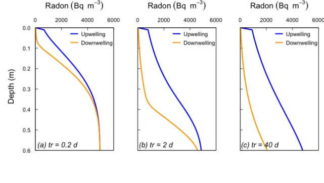
841 842 Figure 4. Sensitivity of radon profiles to recirculation times (tr). Upwelling and 843 downwelling profiles following complete cycles of (a) tr = 0.2 days (reversing every 844 0.1 d), (b) tr = 2 days and (c) tr = 40 days are represented. Note that the results 845 obtained from a recirculation time of 40 days would be equivalent to those 846
37 obtained for larger cycles. Note also that the inflection point in the downwelling 847 profile is similar to the estimated water flux (qv(0)) multiplied by the period of 848 downwelling (tr/2). Other model parameters are the same as in Figure 3. 849 850 Figure 5. Sensitivity of radon profiles in Pz1 to (a) surface water – sediment 851 exchange flux (𝑞!(0)), (b) attenuation of water flux with depth (k), and (c) implicit 852 dispersivity (α). 853 854 Figure 6: Simulated 𝑞! at different depths from 4 different radon profiles that 855 could be accommodated within the analytical uncertainties of radon 856 measurements of Pz1. Orange and grey dots represent lower and upper bounds 857 (1σ), respectively, of the radon measurements. Model parameters are q=0.35, 858 k=0.5, γ=950 (Black line), q=0.35, k = 2, γ=1000 (Blue), q=0.2, k=0.5, γ=820 (Red), 859 q=0.15, k=15, γ=820 (Green). All simulations use θ = 0.4. 860 861 Figure 7. a) Calculated enhanced dispersion coefficient as a function of depth for 862 Pz1 and b) comparison of the water fluxes (𝑞!) at different depths derived from 863 the dispersion approach (circles) and the advective cycling model (solid line). 864 865 866
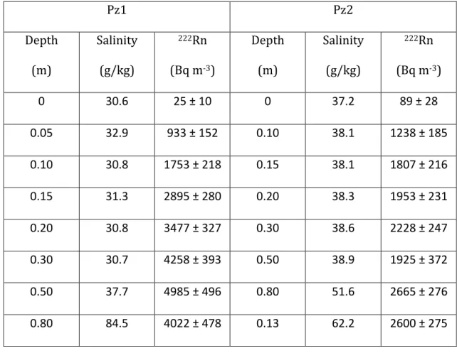
38 Table 1. Measured values of porewater salinity and radon concentration. 867 Uncertainty for radon concentration represents one standard deviation. 868 Pz1 Pz2 Depth (m) Salinity (g/kg) 222Rn (Bq m-3) Depth (m) Salinity (g/kg) 222Rn (Bq m-3) 0 30.6 25 ± 10 0 37.2 89 ± 28 0.05 32.9 933 ± 152 0.10 38.1 1238 ± 185 0.10 30.8 1753 ± 218 0.15 38.1 1807 ± 216 0.15 31.3 2895 ± 280 0.20 38.3 1953 ± 231 0.20 30.8 3477 ± 327 0.30 38.6 2228 ± 247 0.30 30.7 4258 ± 393 0.50 38.9 1925 ± 372 0.50 37.7 4985 ± 496 0.80 51.6 2665 ± 276 0.80 84.5 4022 ± 478 0.13 62.2 2600 ± 275 869 870 871 872
39 873 874 875 876 877 Figure 1. Schematic representation of advective mixing cell model. Arrows denote 878 flow directions during the first phase the recirculation cycle, in which flows are 879 downwards on the LHS and upward on the RHS. (The flow direction is reversed 880 during the second phase of the cycle.) Vertical water fluxes into and out of cell i are 881 qv(i-1) and qv(i), where i = 1,…n, where n+1 is the number of cells in the vertical 882 dimension. The horizontal flux between downwelling and upwelling profiles is 883
denoted qh(i). Concentrations in cell i are ca(i) and cb(i) on LHS and RHS
884 respectively. c(0) is the concentration in surface water. 885 886 887
40 888 889 890 891 892 Figure 2. Observed radon profiles at two different locations within La Palme 893 Lagoon. The error bars represent the analytical uncertainties (1σ) for radon 894 (liquid scintillation counting). 895 896
41 897 898 899 900 901 Figure 3. (a) Mean vertical water velocity (upward or downward), as a function of 902 depth, and resulting radon concentration profile for 𝑡!/2= 10-5 d (0.86 s) for Pz1. 903 The mean vertical water velocity is described by an exponential decrease in depth, 904 according to 𝑞! 𝑧 = 𝑞! 0 𝑒!!". The best-fit to the data is produced with k = 5 m-1 905
and 𝑞! 0 = 0.25 m d-1. Other parameters are γ = 900 Bq m-3 d-1 and θ = 0.4.
906 907
908
42 909 910 911 Figure 4. Sensitivity of radon profiles to recirculation times (tr). Upwelling and 912 downwelling profiles following complete cycles of (a) tr = 0.2 days (reversing every 913 0.1 d), (b) tr = 2 days and (c) tr = 40 days are represented. Note that the results 914 obtained from a recirculation time of 40 days would be equivalent to those 915 obtained for larger cycles. Note also that the inflection point in the downwelling 916 profile is similar to the estimated water flux (qv(0)) multiplied by the period of 917 downwelling (tr/2). Other model parameters are the same as in Figure 3. 918 919
43 920 921 922 923 Figure 5. Sensitivity of radon profiles in Pz1 to (a) surface water – sediment 924 exchange flux (𝑞!(0)), (b) attenuation of water flux with depth (k), and (c) implicit 925 dispersivity (α). 926 927 928
44 929 930 931 932 Figure 6: Simulated 𝑞! at different depths from 4 different radon profiles that 933 could be accommodated within the analytical uncertainties of radon 934 measurements of Pz1. Model parameters are q=0.35, k=0.5, γ=950 (Black line), 935 q=0.35, k = 2, γ=1000 (Blue), q=0.2, k=0.5, γ=820 (Red), q=0.15, k=15, γ=820 936 (Green). All simulations use θ = 0.4. 937 938 939 940
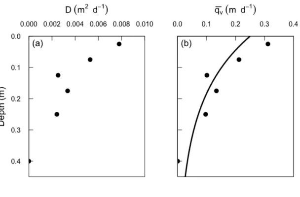
45 941 942 943 944 945 Figure 7. a) Calculated enhanced dispersion coefficient as a function of depth for 946 Pz1 and b) comparison of the water fluxes (𝑞!) at different depths derived from 947 the dispersion approach (circles) and the advective cycling model (solid line). 948 949
![[PDF] Le langage HTML support d'introduction complet |Cours html](data:image/gif;base64,R0lGODlhAQABAIAAAP///wAAACH5BAEAAAAALAAAAAABAAEAAAICRAEAOw==)