HAL Id: insu-00373779
https://hal-insu.archives-ouvertes.fr/insu-00373779
Submitted on 14 Jan 2021
HAL is a multi-disciplinary open access
archive for the deposit and dissemination of
sci-entific research documents, whether they are
pub-lished or not. The documents may come from
teaching and research institutions in France or
abroad, or from public or private research centers.
L’archive ouverte pluridisciplinaire HAL, est
destinée au dépôt et à la diffusion de documents
scientifiques de niveau recherche, publiés ou non,
émanant des établissements d’enseignement et de
recherche français ou étrangers, des laboratoires
publics ou privés.
Similarity of vegetation dynamics during interglacial
periods
Rachid Cheddadi, Jacques-Louis de Beaulieu, Jean Jouzel, Valérie
Andrieu-Ponel, Jeanne-Marie Laurent, Maurice Reille, Dominique Raynaud,
Avner Bar-Hen
To cite this version:
Rachid Cheddadi, Jacques-Louis de Beaulieu, Jean Jouzel, Valérie Andrieu-Ponel, Jeanne-Marie
Lau-rent, et al.. Similarity of vegetation dynamics during interglacial periods. Proceedings of the National
Academy of Sciences of the United States of America , National Academy of Sciences, 2005, 102 (39),
pp.13939 à 13943. �10.1073/pnas.0501752102�. �insu-00373779�
Similarity of vegetation dynamics during
interglacial periods
Rachid Cheddadi*†, Jacques-Louis de Beaulieu‡, Jean Jouzel§, Vale´rie Andrieu-Ponel‡, Jeanne-Marine Laurent*,
Maurice Reille‡, Dominique Raynaud¶, and Avner Bar-Hen储
*Institut des Sciences de l’Evolution, Centre National de la Recherche Scientifique, Unite Mixte de Recherche 5554, 34090 Montpellier, France;‡Institut Me´diterrane´en d’Ecologie et de Pale´oe´cologie, Centre National de la Recherche Scientifique, Unite Mixte de Recherche 6116, Faculte´ des Sciences de Saint Je´roˆme, Case 451, 13397 Marseille Cedex 20, France;§Laboratoire des Sciences du Climat et de l’Environnement, Commissariat a` l’Energie Atomique兾Centre National de la Recherche Scientifique, 91198 Gif-sur-Yvette, France;¶Laboratoire de Glaciologie et Ge´ophysique de l’Environnement, Centre National de la Recherche Scientifique, B.P. 96, 38402 Saint Martin d’Hye`res Cedex, France; and储Universite Aix-Marseille III, Faculte´ des Sciences et Techniques Saint Je´rôme, Laboratoire d’Analyse, Topologie, Probabilite´s, 13397 Marseille Cedex 20, France
Edited by H. E. Wright, University of Minnesota, Minneapolis, MN, and approved August 10, 2005 (received for review March 3, 2005)
The Velay sequence (France) provides a unique, continuous, pa-lynological record spanning the last four climatic cycles. A pollen-based reconstruction of temperature and precipitation displays marked climatic cycles. An analysis of the climate and vegetation changes during the interglacial periods reveals comparable fea-tures and identical major vegetation successions. Although Marine Isotope Stage (MIS) 11.3 and the Holocene had similar earth precessional variations, their correspondence in terms of vegeta-tion dynamics is low. MIS 9.5, 7.5, and especially 5.5 display closer correlation to the Holocene than MIS 11.3. Ecological factors, such as the distribution and composition of glacial refugia or postglacial migration patterns, may explain these discrepancies. Comparison of ecosystem dynamics during the past five interglacials suggests that vegetation development in the current interglacial has no analogue from the past 500,000 years.
climatic cycles兩 interglacials 兩 pollen records
T
he Pleistocene period recorded important and cyclic climatic changes that were mainly related to variations of the earth’s orbit. The astronomical theory of palaeoclimate describes the changes in insolation received by the earth (1). These changes have had a major impact on the vegetation at different latitudes and longitudes (2). During the 100,000-year (100-ka) climatic cycles, western European vegetation has oscillated between extreme situations: those of the ice ages dominated by a herba-ceous treeless vegetation and those of the interglacial periods where forests occupied greatly extended ranges. The intergla-cials have been periods during which vegetation develops in a manner analogous to the current interglacial, within a similar atmospheric concentration of CO2, reduced ice caps, higher sealevels, and broadly comparable climate. The stability, duration, and correspondence of past interglacials with the Holocene is still a matter of debate, mainly because of the impact of human activities and related anthropogenic greenhouse gases (3).
Thus, to predict and anticipate future climate impacts on ecosystems, it is essential to study past climate changes and their related vegetational successions during previous interglacials. In Europe, the last interglacial period, the Eemian, or marine isotope stage (MIS) 5.5 (4, 5), has been more actively studied than any of the previous interglacials, mainly because of the greater number of sites with corresponding sediment deposits. Although the Eemian appears dissimilar to the Holocene from the point of view of insolation (6), this interglacial is still considered an excellent analogue for studying the changes occurring during an interglacial–glacial transition (7). Loutre and Berger (8) stressed that, during MIS 11.3, the earth’s orbit was almost circular, and seasonal insolation changes due to precession were very small. Furthermore, they stated that such changes in the earth’s orbital configuration occurred with a periodicity of⬇400 ka. Thus, in terms of insolation, MIS 11.3 would be the closest analogue to the Holocene.
Here we investigate the similarity of vegetation changes and related climate during the last five interglacial periods: MIS 11.3, MIS 9.5; MIS 7.5, MIS 5.5, and the Holocene.
Materials and Methods
Many detailed vegetation studies explaining vegetational suc-cession through the interglacials have been conducted in Europe since the first simplified model was suggested by Iversen in 1964 (9, 10). The Velay record allows us to identify ecosystem dynamics specific to each interglacial period. The Velay se-quence, obtained from maar lakes located in the southeastern part of the French Massif Central (11), represents the longest record available from the western European temperate domain. This continuous sequence spans the last four climatic cycles. The Velay region is a basaltic plateau with trachytic explosion craters that ranges from Pliocene to Pleistocene. These maar lakes yielded a series of lacustrine sequences (the main ones being Lac du Bouchet, Ribains, and Praclaux) that offered an unparalleled palaeoenvironmental record for western Europe. The strati-graphic correlation between Lac du Bouchet and Praclaux was based on the presence in both sequences of a thick tephra layer with similar mineralogical composition and an40Ar兾39Ar age of
275⫾ 5 ka (12). The strong similarities of the pollen data above and below the tephra layer reinforce the correlation between the two records and allowed the construction of a highly reliable composite sequence, the ‘‘Velay record,’’ that spans the last four climatic cycles. Unfortunately, the lack of better dating precludes an independent time scale to correlate with marine or ice records.
Pollen data from the Velay record have been used to recon-struct both vegetation dynamics and related past climate changes. Thus, the reconstructed January temperature (Tjan) and annual precipitation (Pann) were obtained by using the ‘‘best modern analogues method’’(13) (Fig. 1A and B). The compar-ison of vegetation changes over the four climatic cycles was based on bioclimatic affinity groups (BAGs), as defined by Laurent et
al. (14), rather than on single taxa. These BAGs were based on
plant morphology (height and shape of leaves), phenology (deciduous or evergreen), and climatic variables. BAGs have different envelopes for different climate variables (monthly means for diurnal temperature range, ground frost frequency, amount of precipitation, relative humidity, rain frequency, per-centage of sunshine hours, and temperature; an annual value for growing degree days⬎5°C).
This paper was submitted directly (Track II) to the PNAS office.
Abbreviations: ka, thousand years; MIS, marine isotope stage; Tjan, reconstructed January temperature; Pann, reconstructed annual precipitation; BAG, bioclimatic affinity groups.
†To whom correspondence should be addressed. E-mail: [email protected].
© 2005 by The National Academy of Sciences of the USA
ENVIRONMENTAL
Results
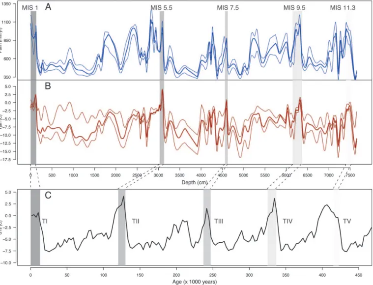
Here, we present reconstructions of climate and vegetation change from the Velay pollen record and compare these changes over the last climatic cycles with a focus on vegetation dynamics during the interglacial periods. The reconstructed Pann and Tjan from the Velay record display a marked cyclic succession of warm and humid interglacials followed by dry and cold glacials (Fig. 1 A and B). During the well defined interglacials, Pann is ⬎800 mm兾year and Tjan is ⬎2°C. During glacial periods, Pann is⬍400 mm兾year and Tjan oscillates between ⫺10°C and ⫺15°C. The four climatic cycles also show obvious similarities in their abrupt terminations where Tjan amplitudes ranged between 12 and 15°C of warming and Pann increased between 600 and 800 mm兾yr.
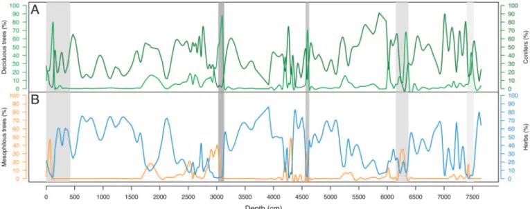
During the interglacials, three BAGs accounted for⬎70% of the pollen content. These BAGs were conifers (BAG 6; Fig. 2A), broadleaved temperate trees (BAG 12; Fig. 2 A) where decidu-ous oaks were the dominant taxa, and mesophildecidu-ous temperate trees (BAG 10; Fig. 2B) with either beech or hornbeam
domi-nant. During the glacial periods, the herbaceous groups of plants (BAGs 22, 23, and 24 dominated by Gramineae, Artemisia and Chenopodiaceae, respectively; Fig. 2B) could exceed 60% of the pollen record.
Discussion
During the last 740 ka, the Earth underwent eight climatic cycles, alternations of ice ages and interglacial periods, with a major shift in the periodicity of these cycles occurring 420 ka ago (15). These climatic cycles were largely triggered by changes in insolation forcing (1). However, recent studies have emphasized the importance of atmospheric CO2concentration in the growth
of global ice volume, particularly at glacial inceptions (16). Despite decreasing insolation since 11 ka, present atmospheric CO2 remains above the values recorded during past glacial
inceptions, preventing ice sheet growth. The modern mismatch between insolation forcing, global ice volume, and atmospheric CO2has not been recorded in any of the previous four climatic
cycles.
Fig. 1. Comparison of reconstructed climate variables from Velay and EPICA records. (A and B) Smoothed annual precipitation and winter temperature reconstructed from the Velay pollen record, respectively. The climatic reconstruction method is based on a search for the best modern analogues (13) among 1,331 spectra from Europe, Northern Asia, and Northern Africa between 10°W兾100°E, and 30°N兾80°N. Forty-six taxa (40 arboreal, 6 nonarboreal) were used to compute the similarity of fossil spectra with modern analogues. The eight most similar modern spectra were included where their chord distance was⬍0.4, a threshold obtained by Monte Carlo simulation. The thin lines represent the upper and lower standard deviations. (C) The surface temperature reconstructed from the ice core record of EPICA (15). Dashed areas correspond to the five interglacials: MIS 11.3, MIS 9.5, MIS 7.5, MIS 5.5, and the Holocene and glacial Terminations TI, TII, TIII, TIV, and TV are reported.
So what does the Velay pollen record tell us about vegetation changes during these past climatic cycles? The reconstructed Tjan and Pann (Fig. 1 A and B) from the Velay pollen record showed similarities during terminations TV to TI and the following interglacials (MIS 11.3, 9.5, 7.5, 5.5, and 1) with those of the European Project for Ice Coring in Antarctica (EPICA) (15) surface temperature record (Fig. 1C). Such similarities are somewhat surprising because there is a well identified lag in global ice volume (a parameter that signals climate change occurring in the Northern Hemisphere) with respect to Antarctic climate during those glacial terminations (17, 18). Without more precise time markers, it is difficult to assess whether such a phase lag also holds true for the Velay record or whether this latter time series is more in phase with the Antarctic record, as it is in the case of global CO2(18). Still, these similarities represent a
global signature in the Velay vegetation changes, at least in a broad sense.
The fact that such similarities were not observed for the glacial inceptions and the following cold periods (Fig. 1C) could be explained by superimposed regional constraints. The impact of long-term and broad scale climate change on vegetation is modulated by ecological factors such as the location of refugia for temperature-dependent taxa during the glacial periods. Climatic conditions during each ice age had a direct impact on the distribution of glacial refugia (2) and subsequent migration routes of taxa in the postglacial periods. Plant composition in the glacial refugia also varied with their geographical extent, the number of species in competition, and the rates of extinction they experienced (2). Some areas in Europe, such as the Iberian, Italian, and Greek peninsulas, the Alps, and the Balkans, were hot spots of biodiversity and sheltered a great number of temperate species during glacial periods (2). The postglacial migration rates from these refugia, also varied, depending on the taxon and its capacity to spread and colonize already occupied areas.
As an example of such ecological impacts, during much of the Eemian (MIS 5.5), hornbeam (Carpinus) dominated the tem-perate deciduous European forest, whereas in the following
interglacial (the Holocene), this taxon has largely by supplanted by beech (Fagus) (9). In southern Italy for earlier interglacials (MIS 13 and 15), other temperate taxa such as the Ulmaceae (Zelkova and Ulmus) had a more significant role (19) than they have for the last four climatic cycles. Today, some of these taxa are present only as relics in a very few isolated areas in Europe. Similar vegetation changes occurred during all of the Quaternary interglacials, but the dominance and兾or composition of taxa from one interglacial to the next were not necessarily due to major climate differences. Earlier studies (10, 11) have investi-gated in detail the taxonomic composition of European pollen records that span climatic cycles. Here, we suggest that the comparison of the broad scale vegetation dynamics over several climatic cycles shows more coherent patterns when it is based on groups of plants, such as BAGs, which have strong climatic affinities, than on single taxa.
Thus, in the Velay record, the succession of broad-leaved temperature trees (BAG 12; Fig. 2 A) by mesophilous temperate trees (BAG 10) marks the climatic optima (Fig. 2B). Similarly, the major development of conifers (BAG 6; Fig. 2 A) and the following periods characterized by herbaceous groups of plants (BAGs 22, 23, and 24) mark the inception of glacial periods (Fig. 2B). After each glacial period, forest recolonization started from an open landscape with pioneer tree taxa.
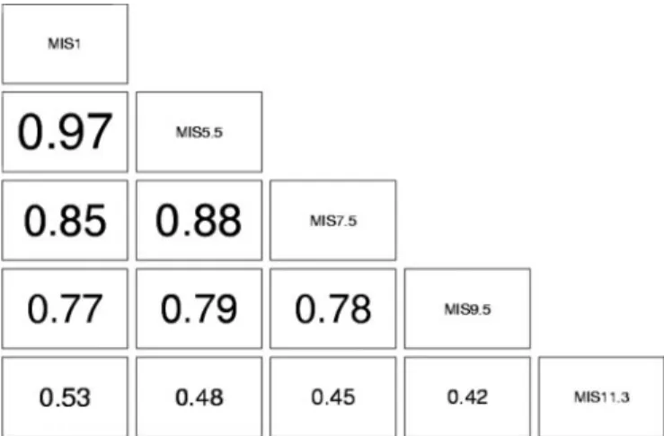
The following vegetation dynamics were apparent from an examination of the interglacial periods (Fig. 3 A–E, dashed areas): (i) BAG 6 decreased and BAG 12 increased at the beginning of each interglacial; (ii) the decrease of BAG 12 when BAG 10 increased marks the end of the climate optima of each interglacial; and (iii) the decrease in values to⬍5% for both BAGs 12 and 10, whereas BAG 6 strongly reincreased, marks the end of each interglacial period. MIS 11.3 (Fig. 3E) was the most divergent interglacial among subsequent interglacials in terms of BAG values. BAG 6 had rather high values during the postglacial period, and BAG 12 showed comparatively ‘‘low’’ percentages (⬍60%) during the beginning of the interglacial and BAG 10 hardly reached 40%. Pearson correlation coefficients between each pair of interglacial periods (Fig. 4) showed that MIS 9.5, 7.5,
Fig. 2. Smoothed curves of bioclimatic affinity groups (BAGs) based on pollen percentages (14). BAG 6 in dark green (A) is composed of Picea abies, Pinus, Pinus
sylvestris; BAG 12 in light green (A) is composed of Alnus, Alnus glutinosa, Corylus avellana, Quercus, Q. robur, Populus, Tilia; BAG 10 in orange (B) is composed
of Acer campestre, Carpinus betulus, Fagus sylvatica, Tilia platyphyllos; and a sum of herbaceous groups in blue (B): BAG 22 (Asteraceae asteroideae, Asteraceae cichorioideae, Gramineae, Myriophyllum, Umbelliferae), BAG23 (Anthemis, Artemisia, Bidens, Brassica, Calystegia sepium, Carduus, Euphorbia, Hypericum,
Knautia arvensis, Lamium, Lysimachia, Lythrum, Papaveraceae, Plantago, P. major, Polygala, Potentilla, Sedum, Stachys), and BAG24 (Caltha, Cardamine,
Caryophyllaceae, Cerastium, Chenopodiaceae, Chenopodium, Cruciferae, Polygonaceae, Polygonum, Ranunculaceae, Ranunculus, Stellaria, Thalictrum). Dashed areas correspond to MIS 11.3, MIS 9.5, MIS 7.5, MIS 5.5, and the Holocene.
ENVIRONMENTAL
and 5.5 were closer analogues to the Holocene than MIS 11.3. In terms of vegetation dynamics, MIS 5.5 displayed the highest correlation coefficient (0.97) with the Holocene, whereas MIS 11.3 was the most different (Fig. 4). On the contrary, vegetation dynamics were not highly distinct between MIS 5.5, 7.5, and 9.5. Analogous forest development during these interglacial periods has already been reported for southern Europe (10).
During the last postglacial period, BAG 6 crossed BAG 12 ⬇12.5 ka ago (Fig. 3A). The uppermost part of the Velay record (modern) showed an initial increase of BAG 6 with very low values of BAGs 10 and 12.
Do such BAG patterns signal the end of the Holocene, as previous interglacial periods might suggest (Fig. 3 B–E)? The variations of orbitally driven insolation during MIS 11.3 have been similar to those existing since ⬇5 ka ago, and they will remain comparable over the next 60 ka (20). The atmospheric CO2record revealed by ice cores during MIS 11.3 showed values
similar to those of the preindustrial period (21). However, one major difference between the present-day situation and MIS 11.3 is the increasing impact of man on the ecosystems. The ice core record during the Holocene provides an important clue in this regard, highlighting a large increase of ⬇30% in atmospheric CO2concentration during the industrial era (from 280 ppmv
around 1750 to 365 ppmv in 1998). This finding clearly reflects the anthropogenic human impact on the global carbon cycle.
Before the preindustrial period, the record indicates a progres-sive increase of⬇20 ppmv between 8 ka and 2 ka (22).
Until recently, it was accepted that this moderate increase was caused by natural changes in continental and oceanic reservoirs. Another possible cause that has now to be taken into account is the increasing human population, whose impact on the climate system may have started as early as 8 ka ago with agricultural practices (23). Nevertheless, present day estimates of anthropo-genic CO2emissions from land use, and the delta13CO2in the
ice core record, indicate that the preindustrial human activities only account for an increase of a few ppmv of CO2 in the
atmosphere (24).
Climate simulations taking into account insolation and various scenarios of atmospheric CO2suggest that the present
intergla-cial period may last ⬎50 ka (16, 23). The cause of such an exceptionally long interglacial is directly related to the modern high concentrations of CO2, which prevent the growth of ice
sheets (16). To enter a glacial period, the atmospheric concen-tration of CO2should decrease, and that decrease should be in
phase with insolation changes (16). According to Ruddiman (3, 23), a glacial inception that should have occurred 5 ka ago has been delayed by human activities beginning at least 3 ka before that time (23).
The Velay pollen record clearly shows that a similar pattern of replacement of BAG 10 by BAG 6 has occurred throughout all
Fig. 3. The last five interglacials. (A–E) BAG percentages reconstructed for the Holocene, MIS 5.5, MIS 7.5, MIS 9.5, and MIS 11.3 from the Velay pollen record. The dark green, light green, and orange curves correspond to BAG 6, BAG 12, and BAG 10, respectively. (A1–E1) Comparison of the winter temperature in dark red and the annual precipitation in blue reconstructed from the Velay pollen record. The three dashed areas represent the beginning of each interglacial (increase of BAG 12 and decrease of BAG 6), the end of each climatic optimum (increase of BAG 10 and decrease of BAG 12), and the end of each interglacial (decrease of BAG 10 and increase of BAG 6).
five interglacials, including the Holocene. Thus, whether the Holocene CO2increase occurred naturally (22) or not
(Ruddi-man’s ‘‘tortoise’’ hypothesis; ref. 23), anthropogenic impacts seem not to have substantially affected the overall vegetation dynamics during the past 8 ka. At least, human activities between 8 ka and 2 ka did not disturb the main vegetational successions. Now, if the anthropogenic increase of CO2has already delayed
a glacial inception (16, 23) then, in terms of ecosystems changes, none of the previous interglacial periods may be considered a predictor of the future. Instead of the expansion of BAGs 22, 23, and 24 (Fig. 2B), as observed at the end of the previous interglacial periods, will BAG 6 (the conifers) dominate the landscape during the next 16–18 ka, until the next ‘‘natural’’ warm period? Will some other BAG succession take place?
Conclusions
The lack of absolute dates in the Velay record does not allow us to discuss the duration of the interglacial periods before the Holocene. However, the pollen data clearly demonstrate that, whatever the duration of these interglacial periods was, the vegetational successions of MIS 11.3, 9.5, 7.5, 5.5, and the Holocene were very similar. This finding raises some questions: 1. Did similar ecosystem dynamics take place during the five interglacials regardless of the amplitude of the insolation and the level of atmospheric CO2? In such a case, is the expansion
of forests in Europe just a matter of interglacial pace? Do the forests expand faster during short interglacials and slower during longer ones? Nevertheless, it is puzzling to have analogous vegetation dynamics during all five interglacials when their durations were (very) different.
2. Does the pattern we observe in the uppermost part of the Velay pollen record indicate the end of the Holocene inter-glacial as it was seen in the previous interinter-glacials? If not, then the Holocene would be a unique interglacial period during which either a reexpansion of BAGs 12 and兾or 10 would take place or the coniferous forests would persist at the temperate latitude for several thousand years until the onset of the next ‘‘natural’’ interglacial period. Such a situation has not been observed during the prior four interglacials.
3. Although insolation values of MIS 11.3 and the Holocene are very similar, their correspondence is not fully recorded in the Velay pollen record. MIS 11.3 displays a different ‘‘ampli-tude’’ in the different BAGs. The long-term vegetation dynamics match the pace of the global insolation changes, but the amplitude of these changes is not linear.
We thank the anonymous reviewers who helped to improve substantially the manuscript. John Keltner has kindly and patiently offered sugges-tions regarding the English. We thank Andra, the French National Radioactive Waste Management Agency, for the financial support it provided within the frame of its geoprospective program under contract 02-60-90. R.C. thanks the Free Software Foundation and the computer scientists who made available theRsoftware (www.r-project.org) under the GNU兾Linux General Public License. This is an ISEM contribution 2005-066.
1. Berger, A. (1978) Quat. Res. 9, 139–167.
2. Bennett, K. D., Tzedakis, P. C. & Willis, K. J. (1991) J. Biogeogr. 18, 103–115. 3. Ruddiman, W. F. (2005) Q. Sci. Rev. 24, 1111–1121.
4. Mangerud, J., Sonstegaard, E. & Sejrup, H. P. (1979) Nature 277, 189–192 . 5. Shakleton, N. J., Sanchez-Goni, M. F., Pailler, D. & Lancelot, Y. (2003) Global
Planetary Change 36, 151–155.
6. Berger, A. & Loutre, M. F. (2002) Science 297, 1287–1288.
7. Kukla, G. J., Bender, M. L., de Beaulieu, J. L., Bond, G., Broecker, W. S., Cleveringa, P., Gavin, J. E., Herbert, T. D., Imbrie, J., Jouzel, J., et al. (2002)
Q. Res. 58, 2–13.
8. Loutre, M. F. & Berger, A. (2003) Global Planetary Change 36, 209–217. 9. Reille, M. & de Beaulieu, J. L. (1995) Q. Res. 44, 205–215.
10. Tzedakis, P. C., Andrieu, V., de Beaulieu, J. L., Birks, H. J. B., Crowhurst, S., Follieri, M., Hooghiemstra, H., Magri, D., Reille, M., Sadori, L., et al. (2001)
Q. Sci. Rev. 20, 1583–1592.
11. Beaulieu, J. L. de & Reille, M. (1984) Boreas 13, 111–132.
12. Roger, S., Fe´raud, G., de Beaulieu, J.-L., Thouveny, N., Coulon, C., Cocheme´, J. J., Andrieu, V. & Williams, V. (1999) Earth Planetary Sci. Lett. 170, 287–299. 13. Guiot, J. (1990) Palaeogeogr. Palaeoclim. Palaeoecol. 80, 49–69.
14. Laurent, J. M., Bar-Hen, A., Franc¸ois, L., Ghislain, M. & Cheddadi, R. (2004)
J. Veg. Sci. 15, 739–746.
15. EPICA Community Members (2004) Nature 429, 623–628. 16. Loutre, M. F. (2003) Earth Planetary Sci. Lett. 212, 213–224.
17. Sowers, T., Bender, M., Raynaud, D., Korotkevich, Y. S. & Orchado, J. (1991)
Paleoceanography 6, 669–696.
18. Petit, R. J., Jouzel, J., Raynaud, D., Barkov, N. I., Barnola, J. M., Basile, I., Bender, M., Chappellaz, J., Davis, M., Delaygue, G., et al. (1999) Nature 399, 429–436.
19. Russo-Ermolli, E. & Cheddadi, R. (1997) Geobios 30, 735–744. 20. Loutre, M. F. & Berger, A. (2000) Climate Change 46, 61–90.
21. Raynaud, D., Barnola, J.-M., Souchez, R., Lorrain, R., Petit, J.-R., Duval, P. & Lipenkov, V. Y. (2005) Nature 436, 39–40.
22. Indermu¨hle, A., Stocker, T. F., Joos, F., Fisher, H., Smith, H. J., Wahlen, M., Deck, B. Mastroianni, D., Tschumi, J., Blunier, T., et al. (1999) Nature 398, 121–126.
23. Ruddiman, W. (2003) Climate Change 61, 261–293.
24. Joos, F., Gerber, S., Prentice, I. C., Otto-Bliesner, B. L. & Valdes, P. J. (2004)
Global Biogeochem. Cycles 18, doi:10.1029兾2003GB002156.
Fig. 4. Pearson correlation coefficients between interglacials. The size of the coefficients are proportional to their value. The five periods were rescaled, and the data were smoothed with splines. For each period, the three BAG percentages were synthesized by principal component analysis, where the first axis represents the linear combination of the percentages that conserve most of the initial variance of the data. The results are very stable among the periods: the first axis accounts for between 65% and 70% of the variance and mostly opposes BAG 6 to BAG 12. Pearson correlation coefficients were computed on pairs of these first axes to quantify the linear link between interglacials.
ENVIRONMENTAL