Wave shapes in alternating DSC

(1)

Journal of Thermal Analysis, Vol. 49 (1997) 1097-1104

WAVE SHAPES IN ALTERNATING DSC

B. S c h e n k e r 1., G . W i d m a n n 2 a n d R . R i e s e n 2 1TCL, Eidgen6ssische Technische Hochschule, CH-8092 Ziirich 2Mettler-Toledo AG, Analytical, CH-8603 Schwerzenbach, Switzerland

Abstract

ADSC with its periodical temperature programs combines the features of DSC measured at high heating rate (high sensitivity) with those at low heating rate (high temperature resolution). In addition, the "reversing" cp effects can be separated from the "non-reversing" latent heat effects. Various periodical temperature programs can be applied. This paper compares the different possible temperature programs and their algorithms for the Cp determination for metal, metal ox- ide and polymer of various properties.

Simulated and measured results for various wave shapes and samples are presented. The rele- vant sample properties and their influence on the measurements are identified and guiding rules for the proper choice of the various experimental parameters are given. Measurements with different samples, performed with the new METTLER TOLEDO STARe-System, are shown and compared with the simulation results. The simulations and the measurements clearly show that the alternating techniques can yield new information about sample properties, but are susceptible to the proper choice of the various experimental parameters.

Keywords: cp-determination, temperature modulated calorimetry, wave shapes

Introduction

Determination of Cp values by DSC is a well established method [1]. The classi- cal method of cp determination employs three DSC runs with a linear temperature profiles. With these three runs, one with an empty pan, one with a well-known reference substance and one with the sample to analyse, the heat capacity can easily be determined. However, this method has the following substantial drawbacks: It depends crucially on the long-time stability of the baseline of the instrument between the three runs and does not allow to measure the Cp value during quasi-iso- thermal conditions. In order to avoid these problems, different dynamic methods were developed. All these methods use different non-linear temperature profiles and sophisticated mathematical methods to compute the Cp values. The Modulated DSC (MDSC) employs a sinusoidal temperature profile and a discrete-Fourier- transformation-based evaluation, the Dynamic DSC (DDSC) uses a piece-wise linear temperature profile and also a Fourier-transformation based evaluation, whereas * Author to whom all correspondence should be addressed.

0368-4466/97/$ 5.00 John Wiley & Sons Limited

(2)

1098 SCHENKER et al.: ALTERNATING DSC

the steady-state DSC (SSADSC) chooses a piece-wise linear temperature profile and pseudo-steady-state evaluation. These three different methods are available in software and hardware options as commercially available instruments, the MDSC from TAI, the DDSC from Perkin-Elmer and the SSADSC from Met-tier-Toledo. This paper compares the three methods for dynamic Cp determination by simulating the instrument and the sample quite rigorously. Although the simulated instrument is of the heat-flow type, all results apply equally for power-compensating instruments.

DSC simulation

In order to keep the simulation simple and the numerical overhead small, the DSC is implemented a linear, time-constant dynamic system. This avoids the diffi- culties of a numerical integration of the system, and allows to employ a more accurate analytical solution of the system of differential equations. Like in [2] the furnace, the sample and the reference holder are modelled as simple RC elements, but here the temperature distribution in the sample is described with a partial differential equation.

Evaluation for Cp

The three compared methods use different excitations signals and employ different evaluation algorithms to determine the Cp values. MDSC uses a sinusoidal temperature profile and employs a Fourier transformation:

T T

A = J'(Ts - TR)sin(o)t)dt + i~(Ts - TR)COS(O3t)dt

o o

where i is ~ and 0~=2u/T. The c o of the sample is then calculated as:

(1)

IAsample [ mCpc~ibration

(2)

cp(MDSC) =

msample I Acalibration

I

where [hsample t denotes the heatflow amplitude of the sample, msampte the mass of the sample, [Acalibrationl the heatflow amplitude of a calibration substance and mCpc~,ibrat~o, the mass times the heat capacity of the calibration substance.

DDSC uses a saw-tooth function as temperature profile and a discrete Fourier transform for evaluation. In contrast to the MDSC the Cp evaluation for this method does not compare the amplitudes, but the only real part of the (generally) complex amplitude.

Re (Asample) mCpcalibration (3)

cp(DDSC) = msample Re(Acalibration)

(3)

SCHENKER et al.: ALTERNATING DSC 1099

The calibration run also gives the phase lag of the instrument, which is taken into account by rotating the amplitude vectors such that the complex part of the

Acalibration vanishes.

SSADSC uses also a saw-tooth function as temperature profile and evaluates the cp simply by comparing the different temperature excursions:

cp(SSADSC) = max(Ts - TR)msample- min(Ts - Ta)) sample

mCpealibratioa

(trmx(Ts - Ta) - min(Ts - TR))

calibration

(4)

Results of the simulation

The simulated cp determination methods are compared for different sample substances, aluminium, sapphire and polystyrene with disk diameters of 4 mm, and with polystyrene disks with 3 mm diameter. Table 1 summarises the physical properties of the sample substances. For all three compared methods a run with a 5 rag, 4 mm diameter aluminium disk was used to normalise the method. Based on these calibration factors the runs of the other samples were evaluated. Since the simulation assumes a perfect balanced instrument, no blank line had to be subtracted.

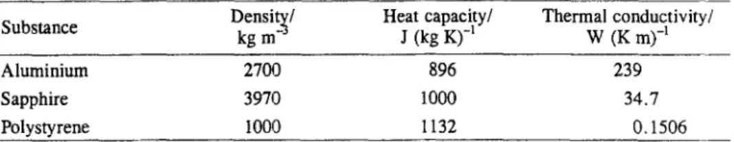
Table 1 Physical properties of the samples investigated

Density/ Heat capacity/ Thermal conductivity/

Substance kg m -~ J (kg K) -1 W (K m) -1

Aluminium 2700 896 239

Sapphire 3970 1000 34.7

Polystyrene 1000 1132 0.1506

Tables 2 to 5 and Fig. 1 summarise the results for the Cp evaluations. For the high heat-conducting sample of aluminum and the heat-conducting sample of sapphire only relatively small errors are encountered, but for the poor-conducting polystyrene disk large errors can be observed, especially for short period durations and relatively large samples. For the parameters recommended by TAI for c o determination using MDSC [3], which recommends 10 to 20 mg of sample and oscilla- tion periods between 60 and 100 s, errors up to 25% for the 4 mm disk and well over 50 % for the 3 mm disk can be observed. Figure 2 shows the temperature distribution in the sample for the 20 rag, 3 mm polystyrene sample. The significant lag of the temperature in the sample can clearly be seen, but due to the linearity of the system and the used excitation of a pure sine wave the measured signal is still a per- fectly looking sine wave.

(4)

Table 2 Relative errors of the Cp evaluations in % for the different methods. Sample: aluminium disks with 4 mm diameter T/s 5 mg sample 10 mg sample 20 mg sample MDSC DDSC SSADSC MDSC DDSC SSADSC MDSC DDSC SSADSC "4 10 0.00 0.00 0.00 -1.79 -1.79 -I .85 -5.18 -5.19 -5.37 20 0.00 0.00 0.00 -1.70 -1.70 -1.70 -4.94 -4.95 --4.93 40 0.00 0.00 0.00 -1.43 -1.43 -1.25 -4.19 -4.21 -3.69 60 0.00 0.00 0.00 -1.13 -1.14 -0.80 -3.34 -3.38 -2.41 80 0.00 0.00 0.00 -0.88 -0.88 -0.47 -2.60 -2.64 -1.44 100 0.00 0.00 0.00 -0.68 -0.68 -0.26 -2.03 -2.06 -0.81 120 0.00 0.00 0.00 -0.53 -0.53 -0.14 -1.60 -1.63 -0.43 160 0.00 0.00 0.00 -0.34 -0.35 -0.04 -1.04 -1.06 -0.12 320 0.00 0.00 0.00 -0.10 -0.10 0.00 -0.30 -0.31 0.00 Table 3 Relative errors of the c o evaluations in % for the different methods. Sample: sapphire disks with 4 mm diameter 5 mg sample 10 mg sample 20 mg sample > ,..] rn T/s MDSC DDSC SSADSC MDSC DDSC SSADSC MDSC DDSC SSADSC 10 20 40 60 80 ₁₀₀ ₁₂₀ ₁₆₀ ₃₂₀ -0.21 -0.21 -0.23 -2.19 -2.20 -2.32 -5.93 -5.97 -6.33 -0.20 --0.20 -0.20 -2.09 -2.09 -2.10 -5.67 -5.69 -5.72 -0.17 -0.17 --0.15 -1.76 -1.76 -1.54 -4.8[ -4.85 -4.26 -0.13 -0.13 -0.09 -1.39 -1.40 -0.99 -3.85 -3.89 -2.79 -0.10 -0.10 -0.05 -1.08 -1.08 -0.58 -3.00 -3.05 -1.67 -0.08 --0.08 -0.03 -0.83 -0.84 -0.32 -2.34 -2.39 -0.94 -0.06 -0.06 -0.02 -0.65 -0.66 -0.17 -1.85 -1.89 -0.51 -0.04 -0.04 0.00 -0.42 -0.43 -0.04 -1.20 -1.23 -0.14 -0.01 -0.01 0.00 -0.12 -0.12 0.00 -0.35 -0.36 0.00 (3

(5)

"lhble 4 Relative errors of the cp evaluations in % for the different methods. Sample: polystyrene disks with 4 mm diameter 5 mg sample 10 mg sample 20 mg sample T/s MDSC DDSC SSADSC MDSC DDSC SSADSC MDSC DDSC 10 -4.45 -7.46 -5.82 -34.54 -48.50 -37.14 -71.24 -79.98 20 -1.55 -2.37 -5.53 -15.48 -23.20 -19.47 -57.31 -69.89 40 -0.70 -0.92 -2.09 -6.33 -9.11 -9.00 -36.50 -49.85 60 -0.46 --0.57 -0.90 -3.82 -5.26 -4.48 -24.43 -35.18 80 -0.33 -0.39 -0.42 -2.62 -3.51 -2.16 -17.26 -25.53 100 --0.25 -0.29 -0.20 -I .91 -2.52 -1.06 -12.72 -19.11 120 -0.19 -0.22 -0.09 -1.45 -1.89 -0.52 -9.69 -14.70 160 -0.12 -0.14 -0.02 -0.90 -1.16 -0.12 -6.07 -9.32 320 -0.03 -0.04 0.00 --0.25 -0.32 0.00 -! .72 -2.68 SSADSC -73.37 -61.03 -38.82 -22.38 -12.73 -6.80 -3.56 -0.94 0.00 z Table 5 Relative errors of the c o evaluations in % for the different methods. Sample: polystyrene disks with 3 mm diameter t-" ,..] T/s 5 mg sample 10 mg sample MDSC DDSC SSADSC MDSC DDSC SSADSC 20 mg sample MDSC DDSC SSADSC 10 20 40 60 80 ₁₀₀ ₁₂₀ ₁₆₀ 320 --25.90 --38.72 --27.77 -66.96 --77.32 -69.59 --9.57 -15.34 --13.25 -49.71 -63.88 -54.09 --3.08 -4.87 -6.18 --27.27 --39.57 --29.56 --1.60 --2.45 --2.59 -16.45 --24.99 -15.09 --1.00 --1.50 --1.13 -10.86 --16.80 -7.68 -0.69 --I.02 -0.51 -7.64 --11.94 -3.68 -0.51 -0.73 -0.23 --5.64 -8.86 -1.76 -0.30 -0.43 -0.05 --3.41 --5.37 -0.40 -0.08 -0.12 0.00 -0.92 --1.46 0.00 -83.66 --88.92 -84.99 -77.12 --83.98 -79.01 --67.54 --77.49 --68.62 -58.81 --71.37 --57.12 --50.75 -64.87 --45.19 -43.59 --58.26 -34.32 -37.40 --51.90 --25.34 -27.72 -40.69 --13.01 -10.20 --16.47 -0.65 C3

(6)

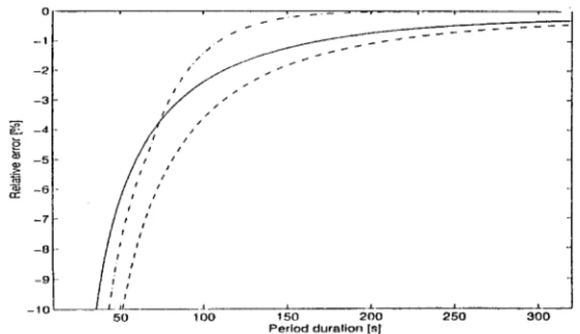
1102 SCHENKER et al.: ALTERNATING DSC 0 - I - 2 -3 ~ - 5 - 7 - 0 - 9 - 10 50 1 O0 150 200 250 300 P e r i o d d u r a l i o n [21

Fig. 1 Comparison of the different methods for a 4 nun polystyrene disk of 10 mg. - - : MDSC, - - - : DDSC, - - - : SSADSC 1 0.8 e ~ 0.6 I / 0 . 4 ~ 0.2 E ~_ - 0 . 2 -0.4 -0.6 - 0 . 8 -1 I10 210 30 40 5to 60 T i m e Is]

Fig. 2 Temperature distribution in a sample of 20 mg o f polystyrene, 60 s period duration. - - : Temperatures o f the different finite elements, - - -: T R, - 9 - : Tp

E x p e r i m e n t a l i n v e s t i g a t i o n s

The heat capacity of polystyrene and sapphire is measured for different period lengths using a sinusoidal temperature excitation with a Mettler D S C 8 2 1 e instru- ment. The polystyrene sample was cut from a plate and had a thickness of 1.34 mm and a footprint of 3x3.5 mm, with a mass of 12.755 rag. The sapphire sample was a circular disc with a thickness of 0.3 mm and a diameter of 4.5 ram, with a mass of 27.245 mg. The measurements are made quasi-isothermally at a temperature of 75~ For each period length four DSC runs with the same crucibles are made:

(7)

SCHENKER et e l . : ALTERNATING DSC 1103

9 An empty run, without crucibles on either the sample nor the reference position.

9 A blank run, with a crucible with a lid on the sample position and a crucible without a lid on the reference position.

9 Two measurements runs with the sapphire, respectively with the polystyrene, samples.

Based on these measurements the heat capacities are computed, using two different algorithms:

Cp(corr.): The empty run and the blank run are employed for calibration of the DSC-cell and for compensation of the cell asymmetry.

cp(conv.): Only the cell asymmetry is compensated.

The calculations are done with the software of the DSC821e.

Table 6 Results of the measurements

Period Measurement Deviation from Measurement Deviation from duration/ polystyrene Cp(corr)/ literature value/ sapphire cp~orr)/ literature value/

S J (g K) -~ % J (g K ) % 20 0.75 -48.9 0.69 -20.2 30 1.00 -31.4 0.78 -10.4 45 1.17 -19.7 0.85 -1.6 60 1.31 -10.0 0.88 1.3 90 1.37 --6.2 0.89 2.5 120 1.38 -5.5 0.88 1.2 180 1.42 -2.3 0.89 2.2 240 1.43 -1.6 0.86 -0.9 1 . 5 1 . 4 1.3 1 . 2 ~-~ 1.1 =~

-g,

0 . 8 0 . 7 O . 6 0 . 5 i = i = i 5 0 1 O 0 1 5 0 2 0 0 2 5 0 P e r i o d d u r a l i o n [s]

Fig. 3 Results of the measurements and the simulation for polystyrene at 75~

I 3 0 0

- - -: literature value polystyrene, 9 9 .: literature value polystyrene - 10%, - - : simulated values, *: Cp(COrr.), x: Cp(COnV.)

(8)

1104 SCHENKER et al.: ALTERNATING DSC

Table 6 and Fig. 3 show the results of single measurements for different period lengths. It can be clearly seen that the relatively thick 1.3 mm polystyrene sample, even with relatively long period durations, shows a Cp value that is significantly too low. The agreement between the simulation and the measurements is satisfactory. The differences can be explained by the fact that the simulation is based on the as- sumption that the heat is transferred only via the base area of the sample and not by the other surfaces. As in the actual measurement the heat is also transferred by the other surfaces, however, this leads to a lower influence of the thermal conductivity. The results for sapphire in Table 6 show that the DSC furnace can readily propagate the modulation down to a period duration of 30 s.

Figure 3 also clearly shows the effect of the correction by the empty and the blank run when Cp(corr) is compared with Cp(COnV). An additional sapphire run is not needed.

Conclusions

Accurate determination of the Cp values in polymers or other poor heat conduc- tors require relatively long period durations in the order of 3 to 6 rain, even if small samples with a large surface and a good thermal contact are used, because for shorter period durations the temperature distribution in the sample is too inhomo- geneous. Note that these period durations are required due to the thermal conductivity in the sample, and not by the dynamics of the employed instrument. Even with an instrument able to use much shorter period durations the sample precludes the application of these shorter durations. For the same accuracy MDSC and DDSC require generally longer period durations. The possibly poor accuracy of the MDSC measurements can not be seen on the measured curves and has to be de- tected by repeated measurements with other period durations. The DDSC method does not fundamentally improve the accuracy but the saw-tooth excitation has a smaller amplitude of the basic frequency used afterwards in the evaluation, for the same temperature scan. The saw-tooth excitation employed in the DDSC and the SSADSC method allow for an easy optical judgement to decide if the period duration is long enough to reach a pseudo-steady state.

From the, somewhat idealised, simulation it can be derived that the SSADSC method yields the most accurate results. In real measurements many other factors like noise, non-linearity, disturbances of the controllers and so forth also influence the results. However, it is to be expected that most of these factors do either not fa- vour any of the methods or affect the SSADSC method only to a lesser degree.

References

1 B. Wunderlich, Thermal Analysis, Academic Press, Boston 1990. 2 U. Ulbrich and H. Cammenga, Thermochim. Acta, 229 (1993) 53. 3 TAI Thermal Applications Note, Heat Capacity by Modulated DSC.