HAL Id: inria-00193551
https://hal.inria.fr/inria-00193551
Submitted on 7 Dec 2007
HAL is a multi-disciplinary open access
archive for the deposit and dissemination of
sci-entific research documents, whether they are
pub-lished or not. The documents may come from
teaching and research institutions in France or
abroad, or from public or private research centers.
L’archive ouverte pluridisciplinaire HAL, est
destinée au dépôt et à la diffusion de documents
scientifiques de niveau recherche, publiés ou non,
émanant des établissements d’enseignement et de
recherche français ou étrangers, des laboratoires
publics ou privés.
Stefanie Hahmann, Alexander Belyaev, Laurent Busé, Gershon Elber, Bernard
Mourrain, Christian Roessl
To cite this version:
Stefanie Hahmann, Alexander Belyaev, Laurent Busé, Gershon Elber, Bernard Mourrain, et al.. Shape
Interrogation. Leila De Floriani, Michela Spagnuolo. Shape Analysis and Structuring, Springer,
pp.1-51, 2008, Mathematics and Visualization, 978-3-540-33265-7. �10.1007/978-3-540-33265-7_1�.
�inria-00193551�
Stefanie Hahmann1, Alexander Belyaev2, Laurent Bus´e3, Gershon Elber4, Bernard Mourrain3, and Christian R¨ossl3
1
Laboratoire Jean Kuntzmann, Institut National Polytechnique de Grenoble, France
MPII, Max Planck Institut f¨ur Informatik, Saarbr¨ucken, Germany [email protected]
3
INRIA Sophia-Antipolis, France
[email protected], [email protected], [email protected]
4
Technion - Israel Institute of Technology, Haifa 32000, Israel [email protected]
Summary. Shape interrogation methods are of increasing interest in geometric modeling as well as in computer graphics. Originating 20 years ago from CAD/CAM applications where ”class A” surfaces are required and no surface imperfections are allowed, shape interrogation has become recently an important tool for various other types of surface representations such as triangulated or polygonal surfaces, subdivi-sion surface, and algebraic surfaces. In this paper we present the state-of-the-art of shape interrogation methods including methods for detecting surface imperfections, surface analysis tools and methods for visualizing intrinsic surface properties. Fur-thermore we focus on stable numerical and symbolic solving of algebraic systems of equations, a problem that arises in most shape interrogation methods.
1 Introduction
Shape interrogation is the process of extraction of information from a geomet-ric model. Surface interrogation is of central importance in modern Computer Graphics and Computer Aided Design (CAD) systems. Wherever geometrical models are used, they often need to be analyzed with respect to different as-pects like, for example, visual pleasantness, technical smoothness, geometric constraints or surface intrinsic properties. The various methods, which are presented in this survey can be used to detect surface imperfections, to ana-lyze shapes or to visualize different forms. We not only restrict the shapes to be investigated to free-form surfaces, but include polygonal meshes as well as algebraic surfaces. Artefacts of subdivision surfaces are subject of Chapter 4 of this book [23]. Particular attention is paid to stable numerical and symbolic
solving of algebraic systems of equations, a problem that arises in most shape interrogation methods.
In Section 2, fundamental notions of differential geometry are briefly re-called. Interrogation methods for polygonal meshes are discussed in Section 3. First and second order shape interrogation and visualization techniques are discussed in Sections 4, 5, focusing mainly on free-form curves and surfaces. The computation and visualization of characteristic curves on surfaces is sub-ject of Section 6. Section 7 discusses the use of robust symbolic computation methods for shape interrogation. Interrogation of algebraic curves and sur-faces is finally discussed in Section 8, in particular the transversal problem of solving of algebraic systems of equations is described.
2 Differential Geometry of curves and surfaces
Fundamental notions of differential geometry of curves and surfaces that are needed in the following of the paper will briefly be reviewed in this section. For a complete bibliography on differential geometry the reader is referred to standard literature [39, 102, 79, 176].
2.1 Curves
A parametric curve is a mapping x from I = [a, b] ⊂ IR into IRn of class Cr(r ≥ 1). x is called regular, if dx
dt(t) 6= 0 for all t ∈ I. If L is the length of
x([a, b]), there exists a unique parameter transformation s from I into [0, L] such that for all t0, t1 ∈ [0, L] the length of the arc x([t0, t1]) is equal to
s(t1) − s(t0). For all t ∈ [a, b] s(t) = Ratkdxdtkdt. s is called the arc length
parameterization. It is a geometric invariant of a curve and is therefore also called natural parameterization.
Let x : [0, L] → IR3, s 7→ x(s) be a regular and naturally parameterized curve of class C3, such that kx′′(s)k 6= 0 for all s ∈]0, L[, then
• v1(s) := x′(s) is called tangent vector of x in s.
• v2(s) := x
′′
kx′′k is called unit normal vector of x in s.
• v3(s) := v1(s) × v2(s) is called binormal vector of x in s,
where × denotes the vector product (cross product) in IR3. {v1(s), v2(s), v3(s)}
form an orthonormal basis of IR3 called the Frenet frame of x in s. The following holds: v1, v2, v3are mappings of class C1, and
v′ 1= κ1v2 v′ 2= −κ1v1 + κ2v3 v′ 3= −κ2v2 where
κ(s) = kx′′k , τ (s) =|x
′, x′′, x′′′|
kx′′k
are mappings of class C1 and C0 respectively. |·, ·, ·| denotes the determinant
of the matrix formed by the three vector arguments. κ and τ are called cur-vature and torsion of the curve x. The curcur-vature measures the deviation of a curve from a straight line, and the torsion measures the deviation of a curve from being planar.
v v v 1 2 3
Fig. 1.Frenet frame.
2.2 Surfaces
A parametric surface is a mapping X from Ω ⊂ IR2 into IR3 of class Cr
(r ≥ 1). X is called regular if for all u = (u, v) ∈ Ω, dXuis an invertible linear
mapping. The two partial derivatives of X in u are denoted by Xu(u) and
Xv(u). The affine subspace TuX := {X(u) + λXu(u) + µXv(u) | (λ, µ) ∈ IR 2
} is called tangent plane to X in u.
The unit normal vector field N is given by N := Xu× Xv
kXu× Xvk
.
The moving frame {Xu, Xv, N } is the Gauss frame. The Gauss frame is in
general not an orthogonal frame.
The bilinear form on TuX induced by the inner product of IR
3 is called
the first fundamental form of the surface. The matrix representation of the first fundamental form Iuwith respect to the basis {Xu, Xv} of TuX is given
by G = (gij) with i, j = 1, 2: µ g11g12 g21g22 ¶ = µ hXu, Xui hXu, Xvi hXv, Xui hXv, Xvi 
where <, > denotes the scalar product. The first fundamental form Iuis
form allows measurements on the surface (length of curves, angles of tangent vectors, areas of regions) without referring back to the space IR3, in which the surface lies.
The linear mapping Lu
Lu : TuX → TuX
x 7→ dNu◦ dX −1
u (x)
is called the Weingarten map.
The bilinear symmetric form IIudefined on TuX by
IIu(x, y) = hLu(x), yi
is called the second fundamental form of the surface X.
Its matrix in the basis {Xu, Xu} of TuX is denoted H = (hij) with i, j =
1, 2: µ h11h12 h21h22 ¶ = µ hN, Xuui hN, Xuvi hN, Xvui hN, Xvvi ¶ . The matrix HG−1 of the Weingarten map L
u is symmetric and real and
therefore it has two real eigenvalues κ1, κ2 with corresponding
orthogo-nal eigenvectors. κ1, κ2 are called principle curvatures of the surface X,
also labeled as κmax, κmin. The product of the principle curvatures K =
κ1· κ2 = det(Lu) = det(H)
det(G) is called the Gaussian curvature and its mean
M = 1
2(κ1+ κ2) = trace(Lu) is called the mean curvature.
Another approach for the principle curvatures is the following: Let A := ∆u · Xu+ ∆v · Xv be a tangent vector with kAk = 1. If we intersect the
surface with the plane given by N and A, we get an intersection curve y with the following properties:
˙y(s) = A and e2= ±N
where e2 is the principal normal vector of the space curve y. The implicit
function theorem implies the existence of this normal section curve. To calcu-late the extreme values of the curvature of a normal section curve (the normal section curvature) we can use the method of Lagrange multipliers because we are looking for the extreme values of the normal section curvature κN with
the condition k ˙y(s)k = 1.
As a result of these considerations we obtain the following. Unless the nor-mal section curvature is the same for all directions there are two perpendicular directions A1 and A2 in which κN attains its absolute maximum and its
ab-solute minimum values. These directions are the principal directions with the corresponding normal section curvatures κ1 and κ2.
For A = A1cos ϕ + A2sin ϕ we get Euler’s formula:
If the principal directions are taken as coordinate axes, Euler’s formula implies the so-called Dupin indicatrix:
κ1(u)2+ κ2(u)2= ±1. (1)
We use the Dupin indicatrices as a tool to visualize curvature situations on surfaces. The Dupin indicatrices at elliptic points (K > 0) are ellipses, at hy-perbolic points (K < 0) pairs of hyperbolas, and at parabolic points (K = 0) pairs of parallel lines. Flat points (κ1= κ2 = 0) are degenerated parabolic
cases. Points with κ1= κ2are called umbilical points.
3 Interrogation of discrete shapes
Polygonal meshes constitute the primary tool for 3D surface representation and are frequently used in a wide range of scientific applications, including computer graphics, visualization, and numerical simulations. Two fundamen-tal questions of surface approximation by polygonal meshes concern approx-imation quality (accuracy) [60] and the relation between the accuracy and size of the approximation [61]. Recently both of these questions were also addressed in [29] where a variational approach for surface approximation by polygonal meshes was developed. Shape approximation with polygonal meshes is discussed in more detail in Chapter 2 of this book [1].
Accurate estimation of geometric properties of a surface from its discrete approximation is important for many applications. Nevertheless there is no consensus on how to achieve accurate estimations of simple surface attributes such as the normal vector and curvatures [122]. An accurate polygonal approx-imation of surface geometry in a least-squares sense [60, 29] does not guarantee accurate approximations of surface normals and curvatures by their discrete counterparts [121, 132, 119, 14]. Thus, deriving accurate, consistent, and nu-merically robust estimates for the surface normal vector and curvature tensor remains an area of active and creative research today.
3.1 Surface Normal Estimation
Given a smooth surface approximated by a dense triangle mesh, an accurate and robust estimation of vertex normals is important for a number of tasks including smooth shading [66, 156], curvature estimation (see, e.g., [180]), and feature extraction (see, e.g., [87]).
Usually the normal vector at a vertex of a triangle mesh is estimated as the normalized weighted sum of normals of the incident facets (triangles). A survey of various methods to estimate the normal vector can be found in [174]. Uniform (equal) weights are justified in [63] via finite difference ap-proximations. In [180] the weights are chosen to be equal to the areas of the
incident triangles. Weighting by the inverse areas was considered in [174, 87], and weights equal to the facet angles at the vertex are proposed in [185]. A weighting scheme assuming that the mesh locally approximates a sphere was developed in [120]. The vertex normal vector can be also obtained from the mean curvature vector and, therefore, mean curvature vector estimates pro-posed in [37, 122] lead to approximations of the vertex normals. A standard approach for testing and comparing various methods to estimate surface nor-mals and curvatures consists of tessellating known (analytical) surfaces and comparing the estimates from the resulting mesh and from the original surface [73, 180, 104, 32, 122]. An interesting statistical approach was recently pro-posed in [125, 126]. First steps towards a rigorous mathematical analysis and comprehensive comparison of various weighting schemes are made in [106].
3.2 Curvature Tensor Estimation
Estimates of the curvature tensor on polygonal meshes are applied in a variety of applications ranging from the detection of surface defects to the detection of features. Many techniques have been proposed (see, e.g., [153] for a recent survey), in this section we provide an overview of different approaches.
In order to estimate the curvature tensor at a vertex a certain neighbor-hood of this vertex is considered, typically its 1-ring. A common approach is to first discretize the normal curvature along edges. Given is an edge (i, j), vertex positions Xi, Xj, and the normal Ni, then
κij = 2h(X
j− Xi), Nii
kXj− Xik2
(2)
provides an approximation of the normal curvature at Xiin the tangent
direc-tion which results from projecting Xiand Xjinto the tangent plane defined by
Ni. This expression can be interpreted geometrically as fitting the osculating
circle interpolating Xiand Xj with normal Niat Xi(cf. [130]). Alternatively,
the equation can be derived from discretizing the curvature of a smooth pla-nar curve (cf. [180]). With estimates κij of the normal curvature for all edges
incident to vertex i, Euler’s formula can be applied to relate the κij to the
unknown principal curvatures (and principal directions). Then approximates to the principal curvatures can be obtained either directly as functions of the eigenvalues of a symmetric matrix ([180, 147]) or from solving a least-squares problem ([130, 122]). Alternatively, the trapezoid rule is applied in [188] to get a discrete approximation of the mean curvature M expressed as the integral over the normal curvatures κN, the Gaussian curvature K is obtained from a
similar integral over κ2
N, then M and K define the principal curvatures. Exact
quadrature formulas for curvature estimation are provided in [107].
Another class of techniques for curvature tensor estimation locally fits a smooth parametric surface patch and then derives the differential quantities from that. This leaves the choice for the surface – typically polynomials of
low degree – the geometric quantities to interpolate or approximate – e.g., the vertex positions in a 1-ring neighborhood – and a projection operator to obtain a parameterization – in general the projection into the tangent plane. A straightforward choice is to consider the quadratic height surface
z(x, y) = 12a20x2+ a11xy + 12a02y2,
for a local coordinate system spanned by the normal Ni (in z-direction)
and two orthogonal tangent vectors (in x- and y-direction) and with origin Xi = 0 [64]. Then the parameters a20, a11, and a02 obtained as a
least-squares solution are the elements of the symmetric matrix defining the Wein-garten map. This can be interpreted as estimating the normal curvature from parabolas rather than circles (as with (2)) and then solving a least-squares system like in [122].
In [189] a quadratic Taylor polynomial of different form is applied, namely X(u, v) = Xuu + Xvv +12u2Xuu+ Xuvuv + 12v2Xvv .
The coefficients of the local least-squares approximating polynomial are the first and second order partials and hence define the fundamental forms. For robustness reasons, an exponential map is used as projection operator rather than a simple projection to the tangent plane.
The use of a cubic approximation scheme which takes into account vertex normals in the 1-ring is proposed in [64]. As the normals themselves are local estimates, this effectively enlarges the neighborhood. Again, a least-squares problem is solved to find the coefficients of a cubic height surface, where the Weingarten matrix is obtained entirely from the quadratic terms in the same way as before.
In general, least-squares methods may suffer from degenerate cases – even for reasonable geometric configurations – which lead to ill-conditioned system matrices. In [189] the polynomial basis is successively reduced in such cases. An alternative is to provide more samples e.g. from linear interpolation. In [24] the patch fitting approach is discussed from an approximation theory point of view including robustness and numerical issues. For high-quality and con-sistent estimation of curvatures and their derivatives, [145] applies a (rather expensive) global fitting of an implicit surface to the surface mesh.
In contrast to the previously mentioned techniques, tensor averaging meth-ods estimate the curvature tensor as an average over a certain region of a polyhedral mesh. In [30] the curvature tensor is derived building upon the theory of normal cycles. This work includes a proof of convergence under cer-tain sampling conditions based on geometric measure theory. The curvature tensor is defined at each point along an edge, and all contributions are inte-grated over a small region, see also [2]. A similar discrete curvature measure is applied in [80].
Alternative approaches locally consider a triangle with given vertex nor-mals. In [167], the directional derivatives of the normal are expressed as finite
differences for every edge of a triangle. The resulting system of six equa-tions is set up from the vertex posiequa-tions (in parameter space) and normals and then solved for the three unknowns of the Weingarten matrix in least-squares sense. The tensors which are obtained per triangle are transformed to a common coordinate system to get a per-vertex average over the 1-ring. The algorithm can be applied with only slight modifications to compute curvature derivatives from the prior result.
In [181] the curvature tensor is estimated as smooth function (rather than a constant value) per triangle. This technique is inspired by Phong shading [156], where the vertex normals are linearly interpolated over the triangle. These interpolated normals are used to define the first and second order par-tials of the unit normal. This yields a piecewise smooth function defining the curvature tensor and elegant expressions for the Gaussian and mean curva-ture. Although this function is in general not continuous over edges of the triangulation, the approximation error is comparable to other approaches. For the estimation at vertices, the error is reduced by taking averages from all incident triangles.
3.3 Applications to Discrete Shape Analysis
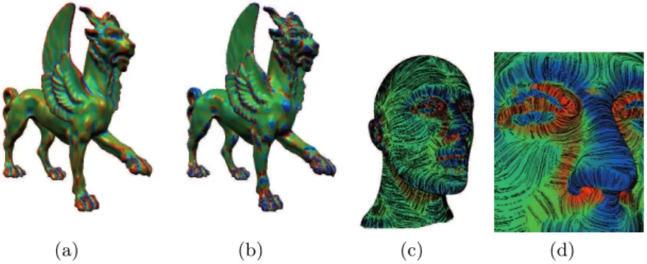
The techniques reviewed in the previous section enable the estimation of cur-vature on discrete shapes: curcur-vature estimates such as principal curcur-vatures, Gaussian curvature and mean curvature are available at every vertex. These values can then be linearly interpolated in triangles. This is illustrated in Fig-ure 2(a) and (b) where M and K are color coded. For efficient visualization (scaled) curvature values are used as 1D texture coordinates such that linear interpolation is done by the graphics hardware. Principal curvature directions
(a) (b) (c) (d)
Fig. 2. Visualization of mean curvature M (a) and Gaussian curvature K (b) estimated on the Feline triangle mesh. Here, red, green and blue denote positive, zero and negative values, respectively, and lighting is enabled. (c) and (d) show the maximum curvature with lines of curvature on the Mannequin mesh.
define a vector field on the surface. Figure 2(c) and (d) shows lines of curvature obtained from stream line integration.
In addition to these examples, many surface interrogation methods which were initially developed for smooth surfaces can be adapted easily to work in the discrete setting. This applies to first order analysis (Section 4) using esti-mates of the surface normal: reflection lines can be simulated by environment mapping techniques, highlight lines and isophotes can be emulated similarly. With curvature estimates being available, second order analysis (Section 5) can be applied. For the computation of discrete characteristic lines (Section 6), curvature derivatives are approximated by appropriate differences.
The following sections discuss shape analysis of smooth surfaces. Interro-gation of discrete shapes follows the general ideas closely and applies estimates of surface normals and curvature.
4 First-Order Shape Analysis
First-order surface interrogation methods make generally use of the surface normal vector by simulation of particular light reflecting behavior of the sur-face. The light reflection methods all simulate the special reflection behavior of light sources or light lines on the surface. Due to the intuitive understand-ing that everybody has when he observes light reflections, these methods are very effective in detecting surface irregularities. They are therefore very well suitable for testing the fairness of surfaces. Because the surface normals are involved in the computation of these lines, they also can be used to visualize first order discontinuities, like tangent discontinuities.
4.1 Reflection lines
The reflection line method determines unwanted dents by emphasizing irreg-ularities in the reflection line pattern of parallel light lines. Let X(u, v) be a representation of the surface to investigate, and let N (u, v) be the unit normal vector of the surface. Furthermore a light line L is given in parameter form:
L(t) = L0+ t · s
where L0 is a point on L, s is a vector defining the direction of L, t ∈ IR.
The reflection line is the projection of the line L on the surface X, which can be seen from the fixed eye point A, if the light line L is reflected on the surface, see Figure 3(a). From geometric dependencies the following reflection condition is derived:
b + λa = 2³N (u, v) · b´N (u, v) with λ := kbk
kak, (3) where a = P − A, b = L − P . Equation (3) has to be solved for the unknown parameters u and v of the reflection point P . These three non-linear equations
reflection line N a b a L 0
(a) Reflectlion line
X N L B E(s) = X + sN highlight line (b) Highlight line L N isophote a = const a (c) Isophote Fig. 3. First order shape analysis by simulating light reflection.
can be reduced to two equations by eliminating λ; they can then be solved by numerical methods, but the existence and uniqueness of solutions has to be ensured by an appropriate choice of the eye point A [94, 98]. To analyze visually the surface one uses a set of parallel reflection lines with direction s, a fixed eye point A, and one steps along each curve of the set. Figure 4(a) shows a reflection line pattern on a part of a hair dryer and visualizes some surface irregularities.
(a) Reflectlion lines (b) Isophotes
Fig. 4. Pattern of computed reflection lines and isophotes on NURBS surfaces.
4.2 Highlight lines
A highlight line is defined as the loci of all points on the surface where the distance between the surface normal and the light line is zero. The linear light source idealized by a straight line with an infinite extension
L(t) = L0+ Bt
(L0 is a point on L, B is a vector defining the direction of L, t ∈ IR), is
posi-tioned above the surface under consideration, see Figure 3(b). The highlight line method also detects surface irregularities and tangent discontinuities by
visualizing special light reflections on the surface. In comparison with the re-flection line method, the highlight lines are calculated independently from any observers view point. For a given surface point X(u, v) let N (u, v) be the unit normal vector. The surface point X(u, v) belongs to the highlight line if both lines, L(t) and the extended surface normal
E(s) = X(u, v) + s · N(u, v) , s ∈ IR intersect, i.e. if the perpendicular distance
d = k[B × N] · [L0− X]k k[B × N]k
between these lines is zero, see Figure 3(b). This method can be extended to highlight bands, lines where d ≤ r (r fixed) is verified. For details on the algorithms to compute highlight lines see [7].
4.3 Isophotes
Isophotes are lines of equal light intensity. If X(u, v) is a parameterization of the surface and L the direction of a parallel lighting, then the isophote condition is given by:
N (u, v) · L = c ,
where c ∈ IR is fixed, see Figure 3(c). Note that silhouettes are special isophotes (c = 0) with respect to the light source. Isoclines are lines of equal normal inclination with respect to some direction V . If X(u, v) is a parameterization of the surface, then the isocline condition is given by:
N (u, v) · V = c
where N (u, v) is the unit normal field of X and c ∈ IR is fixed. In other words, isophotes are isoclines with respect to the light source direction. Similar to reflection lines and highlight lines, the isophotes provide a powerful tool to visualize small surface irregularities, which can not be seen with a simple wire-frame or a shaded surface image. In Figure 4(b) we use 20 different values for c in order to get an isophote pattern on a NURBS test surface.
Now, as stated out in the introduction of this section, the light reflection meth-ods can be used to visualize first and second order discontinuities, because the surface normal vector is always involved in the line definitions. In fact, if the surface is Cr-continuous, then the isophotes are Cr−1-continuous curves (see
[157] for more details). A curvature discontinuity can be recognized, where the isophotes possess tangent discontinuities (breaks). One should nevertheless be careful by using isophotes for this purpose, because sometimes the break points of the isophotes at curvature discontinuities may not be clearly recog-nized, because of an ill-conditioned light direction. This special case occurs if the orthogonal projection of the light direction L in the tangent plane at a
boundary point X(u, v) is parallel to the tangent of the isophote at this point. Isophotes for curvature discontinuity:
There is another isophote method, which on one hand is an automatic method (independent of a special light direction), but which on the other hand only visualizes curvature discontinuities across the boundaries of a patch work. It makes use of the fact that along a common boundary curve y between two surface patches that join only with tangent plane continuity the Dupin indi-catrices i1 and i2 on both sides are different. In general there are two
conju-gate diameters of the Dupin indicatrix. This relation degenerates at parabolic points, because the asymptotic direction (the direction in which the normal section curvature vanishes) is the conjugate to itself, but also conjugate to all other directions. At planar points, we have this degeneration for each (tan-gent) direction. Since both patches have a common boundary curve, and the tangent planes along that curve are unique, the Dupin indicatrices i1, i2have
a common diameter, but differ in the other.
y y t t 1 2 f i1 i2
Fig. 5. Isophotes for curvature discontinuity.
We now consider an isophote c passing through P . The tangent ti of c at P
with respect to Xi is conjugate to the orthogonal projection f of the light ray
onto the tangent plane (i = 1, 2), see Figure 5. In general the isophote c shows a tangent discontinuity at P if the Dupin indicatrices of X1 and X2 are not
equal, but we have to avoid the situations f = ˙y = t and f = t′. More details
can be found in [161].
4.4 Detection of inflections
Orthotomics and the polarity method are both interactive interrogation tools capable to detect only one particular type of surface “imperfection”: the change of the sign in the Gaussian curvature. For example, surface with only convex iso-parameter lines are not necessarily convex, i.e. their Gaussian
cur-vature is not required to be positive at all surface points. Such surface imper-fections are difficult to detect visually in this case and therefore a curvature based surface analysis is needed like color maps or generalized focal surfaces, see Section 5. The following methods in contrast can visualize a change of sign in the Gaussian curvature without computing second order derivatives of the surface.
Orthotomics
In [85] it has been shown that for a regular surface X(u, v) and for a point P that does not lie on the surface or on any tangential plane of the surface the k-orthotomic surface Yk(u, v) with respect to P defined by
Yk(u, v) = P + k
³
(X(u, v) − P ) · N(u, v)´N (u, v) ,
where N (u, v) is the unit normal vector of the surface has a singularity in (u0, w0), if and only if the Gaussian curvature of X vanishes, or changes its
sign at this point. To illustrate this method we consider a B´ezier surface with completely convex parameter lines, see in Figure 6(left). But this surface is not convex: as shown in Figure 6(right), the orthotomic analysis emphasizes the change of sign of the Gaussian curvature in the corner region.
Fig. 6.Bicubic surface patch with line of vanishing Gaussian curvature (left). Or-thotomic analysis (right).
Polarity method
The polarity method is a further method able to detect unwanted changes in the sign of the Gaussian curvature without computing second order derivatives of the surface. It works for curves as well. It uses the polar image of a curve or surface, where the singularities (cusps, edge of regression) of this image indicate the existence of points with vanishing Gaussian curvature. The polar surface looks similar to the orthotomic surface, because the center of polarity is chosen to be equal to the projection point of the orthotomic analysis. For more information about the polarity method and on how removing the inflections see [86].
4.5 Geodesic paths on surfaces and meshes
Geodesic paths, or simply geodesics, on a surface are surface curves which connect two surface points with minimum path length. A thorough study
of geodesics and their role of in surface interrogation requires much more attention than the present overview can provide. So below we give only a brief literature survey.
Geodesics deliver rich information about surface geometry and, therefore, have various theoretical and practical applications. In particular, detecting geodesic paths on surfaces approximated by triangles meshes is a common operation for many graphics and modeling tasks such as mesh parameteriza-tion [103], mesh segmentaparameteriza-tion [93], skinning [175], mesh watermarking [162], and mesh editing [100].
A rigorous mathematical treatment of geodesics can be found in [102, 42]. Some numerical aspects are presented in [56]. An algorithm for approximate computation of geodesic paths on smooth parametric surfaces has been ex-plored in [155, 154]. Various algorithms exit for computing geodesic paths and distances. The so-called MMP algorithm [124] computes an exact solution for the ”single point, all distances” shortest path problem by partitioning each mesh edge into a set of intervals over which the exact distance can be com-puted. In [179] an accelerated implementation of this algorithm is presented. An algorithm to solve the ”single source, single distance” geodesic problem is given in [91]. See also [123] for a broad survey of algorithms for computing shortest paths on graphs.
5 Second-order shape analysis
Surface curvature is of central importance for surface design. Often the result is required to be mathematically smooth (continuous in the 2nd derivative) and aesthetically pleasing, i.e. have smooth flowing highlights and shadows. To obtain an aesthetically pleasing shape, the designer works with the curvature. A color map (see Section 5.5) can be used to visualize curvature (Gaussian, principal curvatures) over the surface. The problem is the good choice of the color scale, which depends on the curvature function and therefore on the underlying surface.
The surface interrogation methods presented in this section are therefore cur-vature analysis tools which are able to detect all surface imperfections re-lated to curvature, like bumps, curvature discontinuity, convexity, and so on.
5.1 Local shape analysis with Gaussian curvature
Let us look at a smooth surface in a neighborhood of one of its point. The simplest classification of local surface shapes is given by the the sign of the Gaussian curvature K = κ1· κ2.
K > 0. The normal curvatures κN(ϕ) has the same sign in all directions, so
concave regions corresponding to this, as demonstrated by the left image of Figure,7 and the left images of Figure 8.
K < 0. The normal curvature becomes zero twice during the half rotation of the normal plane around the normal. The tangent plane intersects with the surface in these directions of zero curvature. The surface is locally saddle-shaped, as seen in middle images of Figure 7 and Figure 8. K = 0. At least one principal curvature is zero. It produces a parabolic point.
See the right image of Figure 7 and the middle-right image of Figure 8. A set parabolic points may form a parabolic region shown in the right image of Figure 8. surface normal surf ace surface normal norm al
k
n< 0k
n> 0 = 0k
n tangent tangent tangent plane plane planeFig. 7. Local shape of normal section curve is defined by curvature.
Fig. 8. Gaussian curvature determines local shape of surface. Left images: convex and concave regions (K > 0). Middle: saddle-shaped region (K < 0). Middle-right: a parabolic point (K = 0) Right: a region consisting of parabolic points.
The Gaussian curvature of a surface can be expressed through the coeffi-cients of the first fundamental form. Thus we arrive at the following famous result called Gauss’s Theorema Egregium: the Gaussian curvature of a surface is a bending invariant.
Now let us consider a simple geometrical interpretation of the Gaussian curvature, by means of which Gauss originally introduced it.
Consider a two-sided surface in three-dimensional space. Let us transport the positive unit normal vector from each point of the surface to the origin. The ends of these vectors lie on the unit sphere. We obtain the mapping of the surface into the unit sphere, see Figure 9. It is called the Gauss map.
The Gauss mapping takes areas on surfaces to areas on the unit sphere. Consider the unit surface normals at the surface points within the area ∆S
on the surface. Let us denote the area on the unit sphere (solid angle) corre-sponding to ∆S by ∆A. It turns out that the Gaussian curvature at the point is the limit of the ratio of these areas:
K = lim
∆S→0
∆A ∆S.
This remarkable formula resembles the definition of the curvature of the plane curves: κ = dϕ/ds.
Gaussian Sphere
Surface Gauss map
S
A A
S
K = lim
Fig. 9. Gauss map and geometric meaning of Gaussian curvature.
The Gauss map can be used for detecting spherical, cylindrical, and conical regions on a surface [12].
5.2 Focal Surface and Corresponding Surface Features For a smooth surface X = X(u, v) its focal surface is given by
XF(u, v) = X(u, v) +
N (u, v)
κ(u, v), κ = κ1, κ2,
where N (u, v) is the oriented normal. The focal surface is formed by the principal centers of curvature and consists of two sheets corresponding to the maximal and minimal principal curvatures κ1 and κ2. One can show that
the focal surface is the envelope of the surface normals. In geometrical optics [77], a caustic generated by a family of rays is defined as the envelope of the family. Thus the focal surface is the caustic of the family of surface normals. The focal surface can be also defined as a surface swept by the singularities of the offset surfaces Od(u, v) = X(u, v) + d N (u, v).
The focal surface is the 3D analogue of the evolute of a planar curve and has singularities. The singularities of the focal surface consist of space curves called focal ribs.
Ridges, the surface curves corresponding to the focal ribs are natural generalization of the curve vertices for surfaces. The ridges can be defined
as sets of surface points where the principal curvatures have extremes along their associated principal directions and points where the principal curvatures are equal (umbilics). A thorough study of the ridges and their properties is conducted by Porteous [158]. See also [72] where a detail classification of the ridges is presented. Below we briefly discuss the ridges from a singularity theory point of view.
Near a point on a focal rib the focal surface can be locally represented in the parametric form (c1t3, c2t2, s), where c1 6= 0 and c2 6= 0, in well chosen
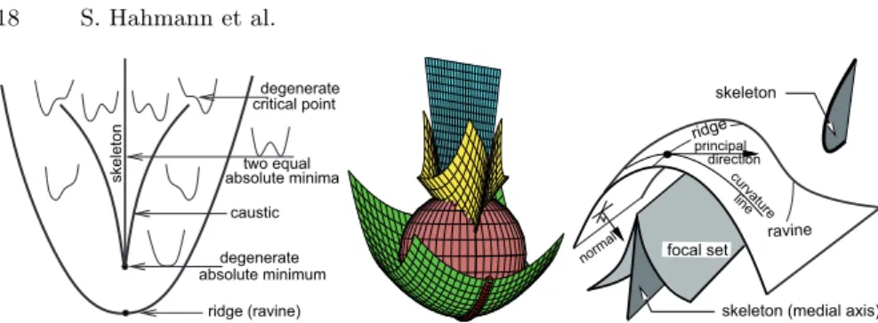
coordinates (s, t). The focal ribs themselves have singularities at points cor-responding to the umbilics and those ridge points where one of the principal curvatures has an inflection along its corresponding curvature line. Generic (typical) singularities of the focal surface are shown in Figure 10.
Fig. 10. Typical singularities of the focal surface. From left to right: cuspidal edge (rib), swallowtail, pyramid, purse. At the swallowtail singularity the rib has a cusp. The pyramid and purse correspond to the umbilical point on the surface. The vertical lines at the bottom images are the surface normals at the corresponding umbilics.
The umbilics and ridge points can be also characterized as surface points where the osculating spheres (spheres of curvature) have high-order contacts with the surface. Therefore the umbilics and ridges are invariant under inver-sion of the surface with respect to any sphere.
The focal surface points can be also described in terms of degenerate sin-gular points of distance functions. Given a surface and a point in 3D, let us consider the distance function from the point and restrict the function onto the surface. This gives a three-dimensional family of distance functions de-fined on the surface and parameterized by points in 3D. Now the focal surface is generated by those point-parameters for which the distance function has degenerate critical points. A typical degenerate critical point has on of the following two forms ±s2+ t3 in proper coordinates s and t. If the
point-parameter is a typical point on a focal rib, the distance function has a critical point in one of the following four forms: ±s2± t4. More degenerate critical
points occur when the point-parameter is located either at a swallowtail sin-gularity of the focal surface or at an umbilical points. It is interesting that the cut locus of the surface [190] (skeleton or medial axis of a figure bounded by the surface) consists of those point-parameters which define the distance functions with two equal global minima. Thus, as illustrated in Figure 11, the edges of the skeleton are located at focal ribs.
ridge (ravine) caustic degenerate degenerate critical point absolute minimum absolute minima two equal skeleto n ravine curva ture line principal direction ridge norma l focal set
skeleton (medial axis) skeleton
Fig. 11.Left: zoo of distance functions; thin lines are used to sketch typical profiles of the surface functions defined by the distance from a given point to the surface points. Center: the skeleton (blue), caustic (yellow), ridge (red) and an osculating sphere (brown) at a ridge point of the elliptic paraboloid. Right: schematic illustra-tion of relaillustra-tionships between the cut locus, focal surface and ridges.
The focal surface possesses many interesting properties. For example, for each line of curvature on a surface there is a corresponding line on the corre-sponding sheet of the focal surface. It can be shown that those raised lines of curvature are geodesics on the focal surface [159, 131].
In [118, 99] umbilics are used for shape interrogation and shape matching purposes. Statistics of various types of umbilics on random surfaces computed and analyzed in [11] may have have many potential applications for for in-specting and interrogating surface properties.
5.3 Hedgehog diagrams and curvature plots
The hedgehog diagrams and curvature plots are well known interrogation tools for planar curves [6, 54]. A hedgehog diagram for planar curves visualizes the curve normals proportional to the curvature value at some curve points. A new curve is obtained by ˜Xhedgehog(t) = X(t) + κN (t) thus visualizing curvature
distribution and discontinuity. The inspection of surfaces with these methods can be done by applying them to planar curves on the surface (intersections of the surface with planes). [97] shows an example of application. Hedgehog diagrams for entire surfaces are nevertheless difficult to interpret and are therefore not to be recommended.
5.4 Generalized focal surfaces
Although the idea of generalized focal surfaces is quite similar to hedgehog diagrams, their application area is much larger. Instead of drawing surface normals proportional to a function value, only the point on the surface nor-mal proportional to the function is drawn. The loci of all these points is the generalized focal surface. This method was introduced by [71], and is based on the concept of focal surfaces which are known from line geometry, intro-duced in Section 5.2. The generalization of this classical concept leads to the
generalized focal surfaces:
F (u, v) = X(u, v) + s · f(κ1, κ2) · N(u, v) , with s ∈ IR
where N is the unit normal vector of the surface X. f is a real valued function of the parameter values (u, v).
The variable offset function f can be any arbitrary scalar function, but in the context of surface interrogation it is quite natural to take f as a function depending on the principal curvatures κ1, κ2 of X, f.ex. f = κ1κ2 Gaussian
curvature, f = 12(κ1+ κ2) mean curvature, f = (κ21+ κ22) energy functional,
f = |κ1| + |κ2| absolute curvature, f = κi principal curvatures, f = κ1i
focal points, f = const offset surfaces. This not only enables to visualize a particular curvature behavior, but it can interrogate and visualize surfaces with respect to various criteria: A convexity test can be performed using the Gaussian curvature offset f = κ1· κ2= K. A surface is locally convex at
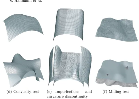
X(u, v), if the Gaussian curvature is positive at this point. Often a surface is called non-convex, if there is a change in the sign of the Gaussian curva-ture. the two surfaces X(u, v) and F (u, v) intersect at the parabolic points, see Figure 12(a). The generalized focal surface therefore pin points directly on the area where the sign of K changes in contrast to orthotomics (Section 4) which are also used to test the convexity. Flat points which are special umbilic points with κ1= κ2= 0 can be detected using f = |κ1| + |κ2| as well
as f = κ2
1+κ22. Flat points are undesired surface points because they make the
surface bumpy. Curvature discontinuity can be visualized through gaps in the surface F with f = κ2
1+ κ22since it is a second order surface analysis tool,
see Figure 12(b). Visualizing surface irregularities: Surfaces are aesthet-ically pleasing if they have “nice” light reflections. Thus similar to reflection lines the generalized focal surfaces are also a tool for visualizing such surface imperfections because they are very sensitive to small irregularities in the shape. In Figure 12(b) part of a hair dryer is shown. It consists of biquintic C1-continuous patches. The iso-parametric lines do not reflect the bump in the
surface, which is however emphasized by the focal analysis. Another aspect of surface analysis is the visualization of technical aspects. A surface which should be treated by a spherical cutter is not allowed to have a curvature radius smaller than the radius of the cutter Rcutter. The generalized focal
sur-faces are able to detect such undesired regions by intersection with the surface X. The offset function to choose in this special case, is f = R 1
cutter − κmax.
Figure 12(c) shows such a surface which is not allowed to be cut. Generalized focal surfaces not only visualize surface imperfections, they also give the user a 3D impression of the relative amount of the offset function over the surface, what color maps can’t do.
5.5 Color mappings
Color is used to emphasize features on the surface. Texturing can emphasize the spatial perception of an 2D image of the surface. A color-coded map is
(d) Convexity test (e) Imperfections and curvature discontinuity
(f) Milling test
Fig. 12. Second order surface analysis with generalized focal surfaces.
an application, which associates to a scalar function value a specific color. The color scale presents an even gradation of color corresponding to the range of function values. Colors are principally used to visualize either continuously or discontinuously any scalar function over a surface [38, 5, 4, 59], like pressure, temperature, or curvature, see Figure 13. Colors are used as a fourth dimension and show the user immediately and quantitatively how the function varies over the surface.
Fig. 13.Color codings of Gaussian curvature.
An even gradation of the linear or cyclic color coding is important to visualize the rapid curvature variation by the presence of color fringes. Beck et al. [5] propose to use the HSI (hue, saturation, intensity) model and to perform
transformations between this space and the three primary colors RGB. See [58] for more details on color spaces and transformations. An example of discrete color-coding of the interval [0,1] is the following one:
Interval Red Green Blue Color 0.0 - 0.2 1 0 0 red 0.2 - 0.4 1 1 0 yellow 0.4 - 0.6 0 1 0 green 0.6 - 0.8 0 1 1 turquoise 0.8 - 1.0 0 0 1 blue
The main difficult of this simple interrogation method is the choice of a con-venient color scale, which obviously depends on the function values to be visualized.
Pseudo texture
The use of colors for displaying a surface helps to emphasize the 3D under-standing of an 2D image by simulating shadows, perspective and depth of the object. An artificial texturing is an aid for visualizing rendered surfaces. Isoparametric lines are commonly used, but they are in some situations am-biguous. Schweitzer [170] projects equally spaced dots of equal size over the surface in order to increase the visual perception of the form.
6 Characteristic lines
Drawing lines on surfaces is a powerful and widely used tool for analysis and visualization of surface features. The techniques of isolines, lines of curvature, geodesic paths and ridges are presented. Numerous graphical examples are illustrated in [159, 56]. In the last three cases a set of lines on the surface can be created, and should be interpreted with the knowledge of differential geometry. They are the most sophisticated tools from the mathe-matician’s point of view. The user should interpret the lines of curvature or the geodesic paths.
6.1 Isolines
Isolines are lines of a constant characteristic value on the surface. They provide an interrogation tool with a wide variety of applications. They help analyzing surface characteristics, and they are used to visualize the distribution of scalar quantities over the surface. The visualization of a certain number of isolines, with respect to an even distribution of the characteristic values allows to study the behavior of these values.
Contour lines are planar lines on the surface which are all parallel to a fixed reference plane. Closed contour lines indicate maxima and minima of the sur-face with respect to the direction given by the plane’s normal vector [76, 5]. Saddle points appear as “passes”. The contour lines only cross in the excep-tional case of a contour at the precise level of a saddle point. [141] describes systematically the distribution of other critical points on a surface. A disad-vantage of contour lines is the fact that they are costly to compute. Several surface contouring methods exist, which are sometimes depending of the spe-cific surface formulation [152, 169, 108]. Hartwig and Nowacki [76] propose to subdivide the surface into sufficient small pieces which are then approximated by bilinear surfaces. Then the contour lines can easily be computed.
Iso-contouring is the technique of extracting constant valued curves and surfaces from 2D and 3D scalar fields. Interactive display and quantitative interrogation helps understanding the overall structure of a scalar field and its evolution over time. Traditional iso-contouring techniques examine each cell of a mesh to test for intersection with the iso-contour of interest. For an overview see [168]. Extraction of isosurfaces from 3D scalar field is generally be done by the Marching Cubes algorithm and its variants [111, 143, 27]
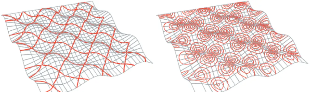
Fig. 14.Gaussian curvature isoline. Left: parabolic lines. Right: isolines correspond-ing to different constant Gaussian curvature values.
Parabolic lines are isolines of zero Gaussian curvature on the surface. They are of particular interest for intrinsic surface interrogation, since they divide the surface into elliptic and hyperbolic regions and they reflect therefore the local curvature behavior of a surface. Parabolic lines are special Gaussian curvature lines, see Figure 14. In [79] a more complex example with the statue Apollo Belvedere is drawn.
6.2 Lines of curvature, umbilics
Lines of curvature are curves whose tangent directions coincide with those of the principal directions, which are orthogonal. They form therefore an orthog-onal net on the surface.
The net of lines of curvature becomes singular at an umbilical point where κ1
and κ2are identical and the principal directions are indeterminate. Some
nu-merical integration method is used to calculate the lines of curvature. But the integration process becomes unstable near an umbilic. Unfortunately umbilics appear frequently on free-form surfaces. A recent work about umbilics [117], destined for use in CAGD (Computer Aided Geometric Design), presents a procedure to compute the lines of curvature near an umbilic. And in [116] a computational method to locate all isolated umbilics on parametric polyno-mial surfaces is described. The discrete field of principle curvature directions computed on a surface mesh has been used for remeshing [2]. More details about umbilics and lines of curvature figures are found in classical differential geometry literature [35], or in a more recent book [159].
6.3 Curvature Extrema for Shape Interrogation
Surface features invariant under rotations, translations, and scaling are impor-tant for studying shapes of 3D objects. The ridge curves discussed briefly in Section 5.2 are among the most important view- and scale-invariant features of a smooth surface.
The ridges are defined as the extremes of the principal curvatures along their corresponding curvature lines and constitute powerful surface descrip-tors. They have been intensively studied in connection with research on the accommodation of the eye lens [69], structural geology [163] and geomor-phology [109], human perception [83], image analysis [191, 129, 127, 40, 110], quality control of free-form surfaces [84], reverse engineering [87], analysis and registration of anatomical structures [68, 67, 151], face recognition [72], and non-photorealistic surface rendering [89, 114, 36]. (See also references therein.) An explanation of why some ridges are good for sketching complex 3D shapes can be found in [191]: given a grey-scale image of an illuminated 3D object, under general illumination and reflection conditions, the zero-crossings of the second directional derivative of the image intensity along the direction of the image intensity gradient occur near the extremes of the principal curvature along their principal directions. Thus the projections of ridges onto the image plane are usually located near edges, the most salient image features.
Some subsets of ridges play an important role in perceptual shape organi-zation. Human perception experiments suggest the so-called minima rule [83] which sets region boundaries along lines divides shapes into parts at negative minima of the principal curvatures along their lines of curvature. The minima rule was employed in [146] for mesh segmentation purposes.
The ridges on a surface have interesting relations with the skeleton (medial axis) of a figure bounded by the surface and can be described via high-order contacts between the surface and its osculating spheres. See [158, 101, 192, 159, 8], [72, Chapter 6], and recent reviews in [26, 25] for rigorous mathematical treatments revealing beautiful properties of these cur-vature features. Surface landmarks associated with the ridges were considered
in [101, 131, 160]. Bifurcations of the ridges on dynamic shapes were studied in [159, 15, 16, 160, 112].
Recently the so-called crest lines, a subset of the ridges consisting of the extremes of the principal curvature maximal in absolute value along its corresponding curvature line, draw much attention because of their ability to represent surface creases [184, 127, 151, 177, 145, 81]. See also references therein. One motivation for describing surface creases as the crest lines is based upon the following analogy with edges of grey-scale images [145]. Consider a surface and its Gauss map which associates with every point p of the surface the oriented normal vector n(p). The derivative ∇n(p) (Jacobian matrix) of the Gauss map measures the variation of the normal vector near p, i.e., how the surface bends near p. It is easy to see that the eigenvalues and eigenvectors of ∇n(p) are the principal curvatures and principal directions of the surface at p, respectively. Thus the maximal variation the surface normal is achieved in the principal direction of the principal curvature maximal in absolute value. So it is natural to define surface creases as loci of points where the positive (negative) variation of the surface normal in the direction of its maximal change attains a local maximum (minimum). Figure 16 shows the crest lines detected on various models represented by dense triangle meshes.
Practical detection of the ridges and their subsets is a difficult computa-tional task since it involves estimating of high-order surface derivatives. Var-ious techniques were proposed for detecting the ridge lines and their subsets on
• surfaces in implicit form and isosurfaces of 3D images [158, 129, 128, 184, 182, 10, 13];
• surfaces approximated by polygonal meshes [113, 9, 188, 82, 177, 26, 25, 145, 81];
• height data [65, 96, 95, 109];
• surface given in parametric form [84, 75].
Fig. 15.Various types of ridges detected on smooth surfaces. The images are taken from [13].
For shape interrogation purposes (shape quality control and analysis of aesthetic free-form surfaces), the ridges were used in [84, 78]. Moreton and
Fig. 16.The crest lines detected on various surfaces approximated by dense triangle meshes.
Sequin [130] used the sum of the squared derivatives of the principal curvatures along their corresponding curvature lines as a measure of surface fairness.
Often, instead of the ridges and their subsets defined via extremes of the principal curvatures, simpler surface features are detected. In geometric mod-eling, there has been considerable effort to develop robust methods for de-tecting surface creases, curves on a surface where the surface bends sharply. Interesting methods for crease detection on dense triangle meshes and point-sampled surfaces were proposed in [87, 166, 88, 70, 178, 148, 150]
Whereas the ridges were first studied one hundred years ago [69] and have rich history [159], the so-called sub-parabolic lines, the loci of points where one of the principal curvatures has an extreme value when moving along the curvature line corresponding to another principal curvature. The sub-parabolic lines were introduced in [17] and studied in [159, 131, 160]. They possess many remarkable properties: the sub-parabolic lines correspond to the parabolic lines on the focal surface, hence the name, and consist of geodesic inflections of the lines of curvature [131]. The sub-parabolic lines can be also detected by examining the profiles of surfaces [131].
6.4 Special Surface Points
In this section, following [131] we consider special surface points which lie on the ridges and sub-parabolic lines. We adapt the color scheme proposed by Porteous [158, 159]. Let us give the principal curvatures and corresponding principal directions, parabolic lines, and sheets of the focal surface a color (red or blue) in order to distinguish between them. The red (blue) sub-parabolic line consists of the extremes of the red (blue) principal curvature along the blue
(red) curvature line. The following surface landmarks are useful for surface interrogation purposes:
• Umbilic points. See [118, 149] for application of umbilics in surface matching and shape interrogation.
• A ridge and sub-parabolic line of the same color cross. The prin-cipal curvature of the same color takes an extreme value there (maximum, minimum, or saddle).
• A ridge is tangent to the line of curvature of the same color. These surface landmarks corresponds to the swallowtail singularities of the focal surface.
• A ridge crosses a ridge of other color. In [183] it was suggested to use these landmarks for 3D image registration.
• A ridge crosses the parabolic line of the same color. The Gauss map has the the so-called pleat singularity at such a point [101].
Koenderink [101] introduced two curvature-based measures of surface cur-vature: the curvedness
C = 2 πln
¡ κ21+ κ22
¢
and the shape index
S = −2 πarctan
κ1+ κ2
κ1− κ2
.
These measures are often more convenient for practical purposes then the standard curvature descriptors {κ1, κ2} and {M, K}, where K and M are the
Gaussian and mean curvatures, respectively. In [142] it was suggested to use local maxima of the curvedness to define surface corner points.
7 Robust Symbolic based Shape Interrogation and
Analysis
Interrogation of polynomial and rational surfaces could be made with the aid of symbolic processing. The advantage of the symbolic approach over sampling of properties, like curvature, at a discrete set of point stems from the ability to analyze the properties globally and provide global (error) bounds. Many properties of free-form geometry are differential and can be derived after ex-ecuting a few basic operations over the polynomial or rational representation of the original interrogated curve C(t) or surface S(u, v), namely: differenti-ations, summations and products. We also assume the availability of a zero set finding tool, an operation that is equivalent to intersecting a polynomial or a rational function with a line in R2(a plane in R3). As a simple example,
consider the curvature field of a planar regular curve C(t) = (x(t), y(t)) that is equal to:
κ(t) = x
′(t)y′′(t) − y′(t)x′′(t)
(x′2(t) + y′2(t))2/3 .
κ(t) is not rational due to the fractional power in the denominator, in the normalization factor. Nonetheless, if one only seeks the inflection points of C(t), only the numerator of κ needs to be considered. Then, the solution of the constraint of
x′(t)y′′(t) − y′(t)x′′(t) = 0 (4) finds all the inflection points in the regular planar curve C(t), if any. In Equa-tion (4), the problem of finding all the inflecEqua-tion points of a planar regular curve was reduced to that of finding a zero set. Differentiation and products were used to compute the inflection points’ constraints.
Differentiation of piecewise polynomials and rationals is well known [28, 53]. Similarly, the addition of two (piecewise) polynomials that share a func-tion space (same order and knot sequence) is realized by simply adding the corresponding coefficients. Two polynomials could be elevated to the same function space via knot insertion and degree elevations; see [28, 53] for more details. Products are the last operator we seek, an operation also required because of the quotient rules over addition and differentiation of rationals. Products are more complex to compute (see [43, 53]) but, clearly, products of piecewise polynomials and/or rationals are piecewise polynomials and/or rationals as well.
In summary, the ability to form a closure and compute a differential prop-erty in the piecewise polynomial and/or rational domains, makes it far simpler and robust to analyze that property. While κ is not rational, its numerator is and so inflection points could be detected as a zero set of x′(t)y′′(t)−y′(t)x′′(t).
For similar reasons, the unit normal N (t) of C(t) is not rational but both κ(t)N (t) and N (t)/κ(t) are rational. Hence, x-extreme points and y-extreme points on C(t) can be identified as
hκ(t)N(t), (0, 1)i = 0, and hκ(t)N(t), (1, 0)i = 0,
and the local maximum curvature locations in C(t) are detectable [45] as the zeros of
d hκ(t)N(t), κ(t)N(t)i
dt ,
yet another rational function.
In [45], points of extreme curvature, or alternatively, inflection points are detected using these schemes. In addition, a scheme to approximate an arc-length reparametrizations for piecewise polynomial and/or rational curves is presented.
In the next section, Section 7.1, we will demonstrate the power of symbolic based interrogation in geometric design, for curvature analysis. In Section 7.2, silhouette curves, isoclines and isophotes curves, and reflection curves are all shown to be reducible to zero set finding. Then, in Section 7.3, we consider the problem of symbolic recognition of simple primitive surface shapes.
7.1 Curvature Analysis
Reexamining the second order differential analysis of parametric surfaces (re-call Section 2), it turns out that given a rational surface S(u, v), the Gaussian curvature K is rational whereas the mean curvature M is not (while M2 is).
In [47], a rational form of (the numerator of) K is symbolically computed and its zeros are used to robustly extract the parabolic lines of the surface. Fig-ure 17 presents one example of computing the parabolic curves for a bicubic surface patch as the zeros of K.
Fig. 17.Left: a free-form B-spline surface is presented, after being subdivided into convex (red), concave (green), and hyperbolic regions (yellow). The parabolic lines (white) separate the regions. Right: presents the function of K(u, v) (in yellow) and its zero set (the parabolic lines).
While M is not rational, one can compute M2as a rational form. Similarly,
the form of κ2
1+ κ22, where κi, i = 1, 2, are the two principle curvatures, is
rational and can capture regions that are highly curved. By subdividing the original surface into regions that prescribe different values of κ2
1+ κ22, one can
separate the surface into regions that could be NC-machined more efficiently with different sizes of ball- and flat-end cutters [44]. Let K0 = κ21+ κ22 at
S0 = S(u0, v0). Then, the normal curvature at S0 is bounded from above by
√
K or an NC ball end cutter of radius 1/√K could be locally fitted to S0
without (local) gouging. Figure 18 shows one such example where a surface is divided into regions of different values of extreme curvature, K = κ2
1+ κ22.
See also Equation (1).
7.2 Silhouette, Isoclines/Isophotes and Reflection lines
The extraction of silhouettes of a free-form surface could be easily reduced to a zero set finding problem. Looking at a rational surface S(u, v) from direction vector V , the silhouettes of S are characterized as the rational constraints of
Fig. 18.Left: a free-form B-spline surface is presented, after being subdivided into regions of different levels of κ2
1+ κ
2
2. Right: presents the rational surface κ 2
1+ κ
2
2and
its contouring (in white) at the different levels.
where N (u, v) = ∂S
∂u ×
∂S
∂v. If the view is a perspective view through point P
(the eye), the silhouettes could be derived as the rational form of hN(u, v), S(u, v) − P i = 0.
Interestingly enough, highlight lines [7] (see Section 4.2), isoclines and isophotes (see Section 4.3) could be similarly reduced to a zero set finding, using symbolic manipulation. Let the unit view direction vector for which isoclines are sought be V . Then, positions on surface S(u, v) that present a normal with a constant inclination angle of α degrees could be characterized
as ¿
N (u, v) kN(u, v)k, V
À
= cos(α),
which is not a rational but could be made into one by squaring both sides as, hN(u, v), V i2− kN(u, v)k2cos2(α) = 0, (5)
at the cost of extraction both the + cos(α) and the − cos(α) isoclines, simul-taneously. Figure 19 shows an example of subdividing a free form surface into regions of steep slopes (more than 45 degrees) and shallow slopes, using iso-clines’ analysis. Such a dichotomy might be desired, for example, in layered manufacturing processing where support is to be added to the geometry only below a certain slope.
Reflection lines (see Section 4.1) can also be reduced to rational zero set constraints as follows. An incoming ray V that hits surface S(u, v) will be reflected in direction r(u, v),
r(u, v) = 2N (u, v) − V hN(u, v), N(u, v)i
hN(u, v), V i . (6) In practice, Equation (6) might be difficult to work with near silhou-ettes (where hN(u, v), V i vanish) and so, in [46], 2N(u, v)hN(u, v), V i −
Fig. 19. Isoclines at 45 degrees from the vertical direction V . Left: the function whose zero set (see Equation (5)) prescribes the isoclines of the surface shown in the right figure is presented. Right: Isoclines also serve to split the surface into regions of slopes (normals) with more than 45 degrees (in thin lines) and regions of less than 45 degrees (in thick lines) with respect to the vertical direction V .
V hN(u, v), N(u, v)i was proposed as a better alternative. In [46], reflection ovals, or reflections of circular curves, were similarly reduced to zero set finding problems.
7.3 Surface Recognition
A fundamental question when analyzing free-form geometry is whether the given curve or surface is of a basic primitive nature. That is, a curve is tested if it is a circle, or a surface is tested if it is a cylinder, or alternatively, a surface of revolution. In [48], these questions are answered using symbolic differential analysis. A rational curve is a circle if its rational squared curvature field, κ2(t) = hκ(t)N(t), κ(t)N(t)i, is constant. In other words, given a B-spline
curve C(t), all its coefficient of the B-spline representation of κ2(t) should be
the same and in fact equal to the square of the reciprocal of the radius of the circle. Alternatively, the evolute curve,
E(t) = C(t) + N (t)/κ(t),
which is also rational, should vanish (along with all its control points) at the circle’s center locations.
A surface called the mean evolute surface, E(u, v) = S(u, v) + N (u, v)
2M (u, v),
where M is the mean curvature (see Section 2.2) is also defined in [48] and was shown to be rational for rational surface S(u, v). If S(u, v) is a circular cone, E(u, v) is reduced to a line, the cone’s center axis. Figure 20 presents two such examples. In [48], the connection is made between rational surfaces
of revolution and rational pseudo-focal surfaces (see Section 5.4) Fu(u, v) =
S(u, v) + κN (u,v)
u(u,v), where κu is the normal curvature of S(u, v) in the u
iso-parametric direction. If the u iso-iso-parametric directions are the latitude lines of the surface of revolution, then Fu reduces to the center axis line of the
surface of revolution. (a) (b)
S(u, v)
E
(u, v)
S(u, v)
E(u, v)
Fig. 20.The mean evolute surface reduces to the center axis line of a circular cone or cylinder. In (a), a polynomial approximation of a cylinder surface S(u, v) with unconventional parameterization is presented along with its mean evolute E(u, v). (b) presents a similar view of a portion of a polynomial approximation of a region of a circular cone along with its mean evolute.
For more information, see the recent book on shape interrogation in geo-metric design and manufacturing [149] that discusses many of the above topics as well as intersection problems, distance queries, curvature properties, and geodesics and offsets curves and surfaces.
8 Interrogation of algebraic curves and surfaces
In this section we will focus on particular geometric models: the algebraic curves and surfaces. We will show how to solve in this context some important shape interrogation problems as singularity detection, intersection problems and offset computation. It turns out that all these problems require at one point to solve an algebraic system of equations, this step being the crucial one. We thus articulate this section mainly on methods that can be applied on these algebraic systems.
Most of the curves and surfaces used in CAGD are given by paramet-ric equations, as defined in Section 2. Planar rational curves in CAGD are typically defined as
x(t) = a(t)
c(t), y(t) = b(t) c(t)
where a(t), b(t) and c(t) are polynomials in the Bernstein basis for rational B´ezier curves or in the B-spline basis for NURBS. Note that the algebraic methods most commonly use polynomials in the power basis and polynomials can be converted from Bernstein basis to power basis. Parametric rational surfaces in CAGD are defined by
x(u, v) = a(u, v) d(u, v), y(u, v) = b(u, v) d(u, v), z(u, v) = c(u, v) d(u, v) where a(u, v), b(u, v), c(u, v) and d(u, v) are polynomials.
Most of the shape interrogation problems for algebraic curves and surfaces can be translated in terms of a system of polynomial equations, as this has been widely illustrated in the previous sections (see also the extensive work of Thomas Sederberg on this topic, e.g. [172]). Consequently, methods for solv-ing polynomial systems are required. The aim of this section is to give a quick overview of such methods. In order to be as much concrete as possible we mention the following two typical problems of shape interrogation that can easily be reduced to polynomial system solving:
Singularity detection. An important problem in CAGD is the detection of singularities of a 3D-surface. If an algebraic surface S is given implic-itly by P (x, y, z) = 0 (that is S = {(x, y, z) ∈ R3; P (x, y, z) = 0}), a point
(a, b, c) on S is singular if ∂P ∂x(a, b, c) = ∂P ∂y(a, b, c) = ∂P ∂z(a, b, c) = 0. It is then
clear that the singular points of S are the common roots of the polynomials P,∂P∂x,∂P∂y,∂P∂z.
Computation of intersection points. Given two parameteric curves, one would like to compute their intersection points. By implicitizing one of the two curves this problem is reduced to finding the real roots of a univariate polynomial which is obtained by substituting the parameterization of a curve into the implicit equation of the second one. Similar approaches can be used to compute curve/surface intersection points and more generally to compute a parameterization of an intersection surface/surface curve. Though we are ma-nipulating objects in dimension 3, the polynomial systems that we consider might involve more that 3 variables. For instance, the intersection of 2 para-metric surfaces involve 4 variables. Therefore, we are not going to restrict the number of variables in the methods that we are going to describe. Hereafter, the variables will be denoted x1, . . . , xn. However, since these systems come
from real geometric modeling problems, we will consider only polynomials with real coefficients.