HAL Id: hal-01806465
https://hal.inria.fr/hal-01806465
Submitted on 2 Jun 2018HAL is a multi-disciplinary open access archive for the deposit and dissemination of sci-entific research documents, whether they are pub-lished or not. The documents may come from teaching and research institutions in France or abroad, or from public or private research centers.
L’archive ouverte pluridisciplinaire HAL, est destinée au dépôt et à la diffusion de documents scientifiques de niveau recherche, publiés ou non, émanant des établissements d’enseignement et de recherche français ou étrangers, des laboratoires publics ou privés.
An exponential timestepping algorithm for diffusion
with discontinuous coefficients
Antoine Lejay, Lionel Lenôtre, Géraldine Pichot
To cite this version:
Antoine Lejay, Lionel Lenôtre, Géraldine Pichot. An exponential timestepping algorithm for diffusion with discontinuous coefficients. Journal of Computational Physics, Elsevier, 2019, 396, pp.888-904. �10.1016/j.jcp.2019.07.013�. �hal-01806465�
An exponential timestepping algorithm
for diffusion with discontinuous coefficients
Antoine Lejay
*, Lionel Lenôtre
†and Géraldine Pichot
‡June 2, 2018
Abstract
We present a new Monte Carlo algorithm to simulate diffusion processes in presence of discontinuous convective and diffusive terms. The algorithm is based on the knowledge of close form analytic expressions of the resolvents of the diffusion processes which are usually easier to obtain than close form analytic expressions of the density. In the particular case of diffusion processes with piecewise constant coefficients, known as Skew Diffusions, such close form expressions for the resolvent are available. Then we apply our algorithm to this particular case and we show that the approximate densities of the particles given by the algorithm replicate well the particularities of the true densities (discontinuities, bimodality, ...) Besides, numerical experiments show a quick convergence.
Keywords: Monte Carlo, Skew diffusions, resolvent kernel, diffusion processes with
discontinuous coefficients.
Highlights:
• We present a new algorithm that simulates diffusion processes with discontinuous diffusive and convective terms.
• Applied to Skew diffusions, we show that the algorithm ensures a correct repartition of the mass.
• The convergence is very fast.
‡Université de Lorraine, CNRS, Inria, IECL, F-54000 Nancy, France ;Contact: IECL, Campus scientifique, BP 70239, 54506 Vandœuvre-lès-Nancy, France ; [email protected]
‡Inria Paris, 2 rue Simone Iff, 75012 Paris ; Université Paris-Est, CERMICS (ENPC), 77455 Marne-la-Vallée 2, France ; Contact: Inria Paris, 2 rue Simone Iff, CS 42112, 75589 Paris Cedex 12 ; [email protected]
1 Introduction
Simulating diffusion processes in media presenting discontinuous characteristics is ubiq-uitous for practical applications. Among them, let us cite (with only a few references) geophysics for inert fluids [11, 18, 25, 37, 41], air [40] and ocean [39]; astrophysics [44]; molecular dynamics [7]; population ecology [8,27]; finance [10,17,43], …
In practice, a diffusion process can be though as the collection of the possible trajectories of particles moving randomly in a medium. This is the path of the Monte Carlo method (also called Lagrangian techniques or particles tracking). For example, the particles may
represent a plume of pollutant in a porous medium with initial concentration 𝐶0. Then the
concentration around any point 𝑦 at time 𝑡 is given by 𝐶(𝑡, 𝑦) = ∫︀ 𝐶0(𝑥)𝑝(𝑡, 𝑥, 𝑦)d𝑥 where
𝑝(𝑡, 𝑥, ·) is the density of the particles at time 𝑡 whose initial position is 𝑥. This density
is known in physics for being solution to the Fokker-Planck (or Kolmogorov Forward) equation {︃ 𝜕𝑡𝑝(𝑡, 𝑥, 𝑦) = 12∇(𝑎(𝑦)∇𝑝(𝑡, 𝑥, 𝑦)) − ∇(𝑏(𝑦)𝑝(𝑡, 𝑥, 𝑦)), 𝑝(𝑡, 𝑥, 𝑦) −−→ 𝑡→0 𝛿𝑥 (1.1) As a result, when one simulates 𝑁 particles starting from 𝑥 whose displacement respects
the dynamics of the operator ℒ = 1
2∇(𝑎∇·) + 𝑏∇·which is the adjoint of
1
2∇(𝑎∇·) + ∇(𝑏 ·)
appearing in equation (1.1), the empirical density 𝑝(𝑁 )(𝑡, 𝑥, ·)of the 𝑁 particles gives an
approximation of 𝑝(𝑡, 𝑥, 𝑦). The concentration of the pollutant can thus be approximated by these Lagrangian simulation [25, 26]. Likewise, many other physical quantities may be computed this way, for example macrodispersion coefficients, breakthrough curves, .... [4,33].
Monte Carlo simulations have several advantages. Among them, • they are really simple to set-up and implement,
• they are completely grid-free,
• they do not suffer from the curse of dimensionality, • they do not introduce artificial numerical diffusion [45].
The challenge is to move the particles in the medium by following as accurately as possible their true dynamics.
The simplest case is when the underlying operator is 1
2𝑎△·+𝑏∇·with continuous coefficients.
In that case, the associated process {𝑋𝑡}𝑡≥0is solution to a Stochastic Differential Equation
(SDE) d𝑋𝑡 =√︀𝑎(𝑋𝑡)d𝑊𝑡+ 𝑏(𝑋𝑡)d𝑡 for a Brownian motion 𝑊 . The distribution of 𝑋𝑡+Δ𝑡
given 𝑋𝑡 is then close to the Gaussian distribution of mean 𝑏∆𝑡 and variance 𝑎∆𝑡. The
addition of the Markov property to that last observation directly leads to approximate
the successive positions at times {𝑘∆𝑡}𝑘=0,...,𝑛 of the stochastic process by using Gaussian
distributions. This method is the so-called Euler-Maruyama scheme [24], which generalizes to SDE the Euler scheme for ODE.
However, in many situations, the Gaussian approximation is no longer valid or leads to bad behaviors [25,39]. This is the case when one faces discontinuities in the diffusivity or considers a process generated by a divergence form operator (Fick’s law, for example). To overcome these problems, several schemes have been proposed so far in the literature (see e.g., [5, 18, 25, 30, 38, 41] among many others). However, some convergent schemes do not always lead to accurate simulations as important physical properties may be lost
as shown by some benchmark tests [31]. In addition, only a few schemes actually deals with a convective term 𝑏 (for example, Random Walk Methods [14,15,29]). In some case, exact simulations techniques, based on rejection-acceptance principle, were developed and allowed to deal with a drift [12,16]. But, they are particularly heavy to implement and computationally excessively costly. They also suffer from a lack of flexibility. The basic functionals vary with the coefficients.
This article presents two contributions.
First, we propose a GEneralized Algorithm based on REsolvent for Diffusion (GEARED), which uses a functional called the resolvent kernel instead of an approximation of the density 𝑝(𝑡, 𝑥, 𝑦) as in the Euler-Maruyama scheme. More precisely, the algorithm uses the resolvent kernel in conjunction with recentered exponential timesteps. This approach is relevant once the resolvent kernel has simple analytic and tractable expressions unlike the density. An important feature of the resolvent kernel is that it keeps the symmetry. We refer to [31] for a list of features with their characterizations. In the case of the Brownian motion, this approach has been studied by K. Jansons and G. Lythe who shown its efficiency to deal with boundary conditions [21–23] (see also [1,2,35]). Here we extend this approach to deal with discontinuities or locally non constant coefficients.
Second, we apply the GEARED algorithm to deal with the simulation in a one-dimensional medium of diffusion processes 𝑋 which are generated by
ℒ = 𝜌 2 d d𝑥 (︂ 𝑎 d d𝑥 )︂ + 𝑏 d d𝑥
where 𝑎 and 𝑏 are piecewise constant. We show that the GEARED completely overcomes the restrictions of some of the schemes mentioned above which are based on the particular form of the density or explicit knowledge of the distribution of the marginal distribution of the process. Indeed, in presence of a two-valued drift, explicit close form expressions for the density could be cumbersome and then hard to use for numerical purposes while the resolvent kernel has an explicit expression [28]. Numerical experiments show that the GEARED algorithm leads to accurate approximations, even in situation where the target density is far to be Gaussian.
The outline of the paper is the following. In Section 2, we present the GEARED algorithm based on an exponential timestepping scheme. In Section 3, we present the implementation of the algorithm for piecewise discontinuous coefficients. Numerical results are given in Section 4. We conclude in Section 5.
2 Context and presentation of the GEARED algorithm
In this section, let us introduce first the assumptions on the coefficients and recall the exponential formula for the resolvent kernel. Then we present the GEARED algorithm.
2.1 Assumptions on the coefficients
Notation 2.1. We denote by 𝒞0(R) the space of continuous functions vanishing at infinities,
by L2(R)the space of square integrable functions on R and by H1(R)the space of functions
Assumption 2.1. 𝑎, 𝜌, 𝑏 are measurable functions from R to R such that
0 < 𝜆 ≤ 𝑎(𝑥), 𝜌(𝑥) ≤ Λ, |𝑏(𝑥)| ≤ Λ for some positive constants 𝜆, Λ.
Let us define ℎ(𝑥) := 2 ∫︁ 𝑥 0 𝑏(𝑦) 𝑎(𝑦)𝜌(𝑦)d𝑦. (2.1)
We set (ℒ, Dom(ℒ)) the infinitesimal generator given by
ℒ := 1 2𝜌(𝑥) d d𝑥 (︂ 𝑎(𝑥) d d𝑥· )︂ + 𝑏(𝑥) d d𝑥 = 1 2𝑒 −ℎ(𝑥) 𝜌(𝑥) d d𝑥 (︂ 𝑎(𝑥)𝑒ℎ(𝑥) d d𝑥· )︂ (2.2) and the domain
Dom(ℒ) = {𝑓 ∈ 𝒞0(R, R) | ℒ𝑓 ∈ 𝒞0(R, R)}.
The two different expressions of the operator above corresponds. The right-hand side of (2.2) is actually the so-called factorized form we are going to introduce later.
The assumptions on 𝑎, 𝜌 and 𝑏 ensure the existence of a unique, Feller process 𝑋 whose infinitesimal generator is (ℒ, Dom(ℒ)). More precisely, 𝑋 is the process whose density
transition function 𝑝(𝑡, 𝑥, 𝑦) derives from the semi-group {𝑃𝑡}𝑡>0associated to (ℒ, Dom(ℒ)).
This is the result of the equality
𝑃𝑡𝑓 (𝑥) =E𝑥[𝑓 (𝑋𝑡)] =
∫︁
R
𝑝(𝑡, 𝑥, 𝑦)𝑓 (𝑦)d𝑦,
for any measurable function 𝑓 which is either bounded or in L2(R).
Consequently, 𝑋 is the continuous stochastic process whose density transition function
𝑝(𝑡, 𝑥, 𝑦) is the solution to Fokker-Planck equation and is thus the process of interest for
the simulation of a diffusion problem. As an illustration, • When 𝑎 = 1, then 𝑋 is the solution to the SDE
𝑋𝑡 = 𝑥 + ∫︁ 𝑡 0 √︀ 𝜌(𝑋𝑠)d𝑊𝑠+ ∫︁ 𝑡 0 𝑏(𝑋𝑠)d𝑠.
• When 𝑎 has some isolated discontinuities with left and right-limits, the process 𝑋 is solution to some SDE with local time (See e.g. [29]).
2.2 Definition of resolvent kernel and reminder of the
exponen-tial formula
Definition 2.1. The resolvent {𝑅𝜆}𝜆>0 of the infinitesimal generator (ℒ, Dom(ℒ)) is the
In practice, the resolvent {𝑅𝜆}𝜆>0 of an infinitesimal generator (ℒ, Dom(ℒ)) is given by
the Laplace transform of the semi-group {𝑃𝑡}𝑡≥0 (see [34, theorem 3.1]). As an equation,
it rewrites
𝑅𝜆𝑓 (𝑥) =
∫︁ +∞
0
𝑒−𝜆𝑡𝑃𝑡𝑓 (𝑥)d𝑡, 𝑓 ∈ 𝒞0(R).
When the semi-group {𝑃𝑡}𝑡≥0 has a density transition function, then according to [28,32]
𝑅𝜆𝑓 (𝑥) = ∫︁ R 𝑟(𝜆; 𝑥, 𝑦)𝑓 (𝑦)d𝑦, for 𝑓 ∈ 𝒞0(R) where 𝑟(𝜆; 𝑥, 𝑦) = ∫︁ +∞ 0 𝑒−𝜆𝑡𝑝(𝑡, 𝑥, 𝑦)d𝑡.
The functional 𝑟(𝜆; 𝑥, 𝑦) is the so-called resolvent kernel or Green kernel.
For small values of 𝑡, 𝑡−1𝑅
1/𝑡 is close to 𝑃𝑡. The semi-group can be reconstructed from the
resolvent through the exponential formula by iterating the application of the resolvent.
Proposition 2.1 (Exponential formula [9,34]). For any 𝑡 > 0 and any 𝑓 ∈ 𝒞0(R),
𝑃𝑡𝑓 = lim 𝑛→∞ (︁𝑛 𝑡𝑅𝑛/𝑡 )︁𝑛 𝑓. (2.3)
2.3 Presentation of the GEARED algorithm
2.3.1 Motivations and notations
Many simulation methods for 𝑋 fix the time step ∆𝑡 and draw a realization of a Markov
chain (𝜉𝑘)𝑘≥0 such that
𝜉𝑘+1 ∼ 𝑝𝜉𝑘(∆𝑡, 𝜉𝑘, 𝑦)d𝑦,
where 𝑝𝑥(∆𝑡, 𝑥, ·) is a parametric family of approximations of 𝑝(∆𝑡, 𝑥, ·) when ∆𝑡 is small,
the parameter being the starting point 𝑥 (this is why it appears twice). With such a
scheme, {(𝑘∆𝑡, 𝜉𝑘)}𝑘=0,...,𝑛 is an approximation of {(𝑘∆𝑡, 𝑋𝑘Δ𝑡)}𝑘=0,...,𝑛.
When the coefficients are regular enough, the simplest yet efficient scheme is the
Euler-Maruyama scheme [24]. In this case, 𝑝𝑥(∆𝑡, 𝑥, 𝑦) is obtained by freezing the values of the
coefficients at the point 𝑥.
When the coefficients are discontinuous, the density 𝑝(𝑡, 𝑥, ·) is no longer well approximated by a Gaussian one. Specific schemes should then be designed. They must ensure the correct repartition of the mass (See [30] and references within). For that purpose, one
should find a proper approximation 𝑝𝑥(∆𝑡, 𝑥, 𝑦)of 𝑝(∆𝑡, 𝑥, 𝑦).
Notation 2.2. We denote by ℰ(𝜆) the exponential distribution of parameter 𝜆 > 0.
2.3.2 The GEARED algorithm
The following result is the cornerstone for the construction the GEARED algorithm and is based on a exponential timestepping scheme. It shows how one can use the resolvent to sample the position of 𝑋 at exponential timesteps.
Proposition 2.2. Let 𝜁 ∼ ℰ(𝜆) be independent of 𝑋. The density of 𝑋𝜁, starting at 𝑋0,
is 𝜆𝑟(𝜆; 𝑋0, ·).
Proof. Let us consider that 𝑋0 = 𝑥. The density of the random variable 𝑋𝜁 is, by
conditioning with respect to 𝜁, for any 𝑓 ∈ 𝒞0(R; R),
E[𝑓(𝑋𝜁)] = ∫︁ +∞ 0 𝜆𝑒−𝜆𝑡E[𝑓(𝑋𝑡)]d𝑡 = ∫︁ +∞ 0 𝜆𝑒−𝜆𝑡 ∫︁ R 𝑝(𝑡, 𝑥, 𝑦)𝑓 (𝑦)d𝑦 d𝑡 = ∫︁ R 𝜆𝑟(𝜆; 𝑥, 𝑦)𝑓 (𝑦)𝑚(𝑦)d𝑦. Thus, 𝑋𝜁 ∼ 𝜆𝑟(𝜆; 𝑥, ·) when 𝑋0 = 𝑥.
To build the exponential the timestepping scheme is now rather simple. Using the
Proposition 2.2, for any function 𝑓 ∈ 𝒞0(R),
E𝑥0[𝑓 (𝑋 (𝑛) 𝑇 )] = 1 ∆𝑡 𝑛∫︁ R · · · ∫︁ R 𝑟(∆𝑡−1; 𝑥0, 𝑥1)𝑟(∆𝑡−1; 𝑥1, 𝑥2) · · · 𝑟(∆𝑡−1; 𝑥𝑛−1, 𝑥𝑛)𝑓 (𝑥𝑛)d𝑥1· · · d𝑥𝑛 =(︁𝑛 𝑇𝑅𝑇 /𝑛 )︁𝑛 𝑓 (𝑥0). (2.4)
An application of Exponential formula (2.3) then yields to
E𝑥0[𝑓 (𝑋
(𝑛)
𝑇 )] −−−→
𝑛→∞ E𝑥0[𝑓 (𝑋𝑇)] = 𝑃𝑇𝑓 (𝑥0).
As a result, for a timestep ∆𝑡 = 𝑇 /𝑛,
𝑋(𝑛)0 = 𝑋0, 𝑋
(𝑛)
(𝑘+1)Δ𝑡 ∼ ∆𝑡 −1
𝑟(∆𝑡−1; 𝑋(𝑛)𝑘Δ𝑡, ·),
where 𝜆 has been replaced by 1
Δ𝑡, provides a reliable approximation of a sample path of 𝑋.
This idea is summarized in Algorithm 1.
Data: An initial position 𝑥 at time 0, a time horizon 𝑇 > 0 and an integer 𝑛 such
that ∆𝑡 = 𝑇 /𝑛 is the timestep.
Result: An approximated path (𝑋(𝑛) 0 , 𝑋 (𝑛) Δ𝑡, . . . , 𝑋 (𝑛) 𝑇 ) of (𝑋0, 𝑋𝑇 /𝑛, . . . , 𝑋𝑇)with 𝑋0 = 𝑥. Set 𝑋(𝑛) 0 = 𝑥. for 𝑖 = 1, · · · , 𝑛 do Sample 𝑋(𝑛)
𝑖Δ𝑡 using the density ∆𝑡
−1𝑟(∆𝑡−1; 𝑋(𝑛) (𝑖−1)Δ𝑡, ·). end return (𝑋(𝑛) 0 , 𝑋 (𝑛) Δ𝑡, · · · , 𝑋 (𝑛) 𝑇 ).
2.3.3 Convergence of the GEARED algorithm
When 𝜆 is large, 𝜁 ∼ ℰ(𝜆) concentrates around its mean value 𝜆−1 = ∆𝑡. We formalize
this point in the next proposition.
Proposition 2.3. Let 𝑇 be a time horizon. With 𝜆 = 𝑛/𝑇 and ∆𝑡 = 𝑇 /𝑛 = 𝜆−1, define
𝜎0 = 0 and 𝜎𝑘+1 = 𝜎𝑘+ 𝜁𝑘, 𝜁𝑘 ∼ ℰ(𝜆), {𝜁𝑘}𝑘≥0 independent.
For any 𝜖 > 0 and any 𝛽 > 0, there exists 𝑛′ large enough such that
P [︂ sup 𝑘=0,...,𝑛 |𝑋𝜎𝑘− 𝑋𝑘Δ𝑡| ≥ 𝛽 ]︂ ≤ 𝜖, ∀𝑛 ≥ 𝑛′. (2.5)
In the above proposition, (𝑋𝜎0, . . . , 𝑋𝜎𝑛) has the same distribution as (𝑋
(𝑛)
0 , . . . , 𝑋
(𝑛) 𝑇 ).
This proves that the vector of successive positions is close to the one of the true positions. With some standard additional work, not done here, it is possible to prove that the family
of linear interpolation of (𝑋(𝑛)
0 , . . . , 𝑋
(𝑛)
𝑇 ) is tight and thus converges to (𝑋𝑡)𝑡∈[0,𝑇 ].
Remark 2.1. Although our algorithm draw a realization of 𝑋𝜁, the exponential time 𝜁
itself is not drawn and not known. Trying to recover the exact time wipes out all the numerical interest of the method has it requires to know the density 𝑝(𝑡, 𝑥, ·), which we want to avoid.
Proof. For the above family {𝜁𝑘}𝑘≥0 of exponential random variables, a martingale
in-equality yields P[𝜁𝑛 ≥ 𝛼] ≤ 𝐾 𝛼𝑛 with 𝜖𝑛 =𝑘=0,...,𝑛sup ⃒ ⃒ ⃒ ⃒ 𝜎𝑘− 𝑘𝑇 𝑛 ⃒ ⃒ ⃒ ⃒ . (2.6)
Thus, 𝜎𝑘 is an approximation of 𝑘𝑇 /𝑛, the 𝑘-th position of the process. In addition,
from [20, Theorem 5.1], for any 𝜏 ≥ 0,
P[𝜎𝑛 ≥ 𝑇 + 𝜏 ] ≤exp (︁ −𝜏 𝑇 )︁ . (2.7)
We fix 𝜏 > 0. Let osc𝑇(𝑓, 𝛿) = sup𝑡∈[0,𝑇 ], |𝑠|≤𝛿|𝑓 (𝑡 + 𝑠) − 𝑓 (𝑡)| be the modulus of continuity
of continuous functions 𝑓 : [0, 𝑇 ] → R. Since the paths of 𝑋 are continuous, for any
𝛽, 𝜖 > 0, there exists 𝛼 > 0 such that P[osc𝑇(𝑋, 𝛼) ≥ 𝛽] ≤ 𝜖. This follows e.g. from
Theorem 8.2 and Theorem 1.4 in [6] on tightness.
Then for any 𝜖 > 0 and 𝛽 > 0, when 𝜏 is such that exp(−𝜏/𝑇 ) ≤ 𝜖, 𝛼 such that
P[osc𝑇 +𝜏(𝑋, 𝛼 ≥ 𝛽] ≤ 𝜖and 𝑛 such that 𝐾/𝛼𝑛 ≤ 𝜖, using (2.6) and (2.7),
P [︂ sup 𝑘=0,...,𝑛 |𝑋𝜎𝑘 − 𝑋𝑘𝑇 /𝑛| ≥ 𝛽 ]︂ ≤ P[𝜎𝑛 ≥ 𝑇 + 𝜏 ] + P[︀|𝑋𝜎𝑘− 𝑋𝑘𝑇 /𝑛| ≥ 𝛽; 𝜎𝑛 ≤ 𝑇 + 𝜏 ]︀ ≤ P[𝜎𝑛≥ 𝑇 = 𝜏 ] + P[osc𝑇 +𝜏(𝑋, 𝜖𝑛); 𝜎𝑛≤ 𝑇 + 𝜏 ]. ≤exp(︂ −𝜏 𝑇 )︂ + P[osc𝑇 +𝜏(𝑋, 𝛼) ≥ 𝛽] + P[𝜖𝑛 ≥ 𝛼] ≤ 3𝜖. This proves (2.5).
3 Application to the case of piecewise constant
coeffi-cients
For the sake of simplicity of the presentation, let us consider coefficients with a discontinuity at 0.
3.1 Definition of knotted operators
Notation 3.1 (Knotting). For two functions 𝑓−, 𝑓+: R → R𝑑, we define their knotting by
(𝑓− ◁▷ 𝑓+)(𝑥) :=
{︃
𝑓−(𝑥) if 𝑥 < 0,
𝑓+(𝑥) if 𝑥 ≥ 0.
(3.1)
For 𝑖 = −, +, let (𝑎±, 𝜌±, 𝑏±) be continuous coefficients over R satisfying Assumption 2.1.
We knot them into
(𝑎, 𝜌, 𝑏) := (𝑎−, 𝜌−, 𝑏−) ◁▷ (𝑎+, 𝜌+, 𝑏+).
Notice that 𝑎, 𝜌 and 𝑏 are continuous on (−∞, 0) and (0, +∞) with left and right limits at 0.
For 𝑖 = −, +., we denote by ℒ± the operator (2.2) with the coefficients (𝑎±, 𝜌±, 𝑏±).
3.2 Reduction to a Drifted Skew Brownian Motion (DSBM)
Let us consider the simulation of the process 𝑋 generated by ℒ◁▷ of the form (2.2) with
the piecewise constant coefficients (𝑎, 𝜌, 𝑏) given by
𝑎(𝑥) := (𝑎− ◁▷ 𝑎+)(𝑥), 𝜌(𝑥) = (𝜌− ◁▷ 𝜌+)(𝑥) and 𝑏(𝑥) = (𝑏−◁▷ 𝑏+)(𝑥), (3.2)
where 𝑎𝑖, 𝜌𝑖 > 0 and 𝑏𝑖 ∈ R, for 𝑖 = 1, 2.
The process 𝑋 is the unique strong solution to the SDE
𝑋𝑡= 𝑥 + ∫︁ 𝑡 0 √︀ 𝑎(𝑋𝑠)𝜌(𝑋𝑠)d𝑊𝑠+ ∫︁ 𝑡 0 𝑏(𝑋𝑠)d𝑠 + 𝑎+− 𝑎− 𝑎++ 𝑎− 𝐿0𝑡(𝑋)
where 𝑊 is a Brownian motion and 𝐿0
𝑡(𝑋) is the symmetric local time of 𝑋 at 0 [29]. It
is equivalent through the change of variables
Φ(𝑥) = 𝑥
√︀𝑎(𝑥)𝜌(𝑥)
(often called the Lamperti’s transform) to the the Drifted Skew Brownian motion (DSBM)
𝑌 = Φ(𝑋) (see [28]) which is the solution to
𝑌𝑡= 𝑥 + 𝑊𝑡+ ∫︁ 𝑡 0 𝑏(𝑋𝑠) √︀𝑎(𝑋𝑠)𝜌(𝑋𝑠) d𝑠 + (2𝛽 − 1)𝐿0 𝑡(𝑌 ) where 𝛽 := √︁𝑎 + 𝜌+ √︁𝑎 + 𝜌+ + √︁𝑎 − 𝜌− ∈ (0, 1) and 𝜃 = 2𝛽 − 1 ∈ (−1, 1).
The DSBM 𝑌 is associated to the coefficients ̂︀ a(︂𝛽,√𝑏+ 𝑎+𝜌+ ,√𝑏− 𝑎−𝜌− )︂ := (︂ (1 − 𝛽) ◁▷ 𝛽, (1 − 𝛽)−1 ◁▷ 𝛽−1,√𝑏− 𝑎−𝜌− ◁▷ √𝑏+ 𝑎+𝜌+ )︂ .
Remark 3.1. The transformation Φ is remarkable as reduce the number of parameters to
deal with. In fact, in order to consider the simulation of the class of processes 𝑋, we only have to consider the simulation of the process 𝑍 whose coefficients are
̂︀
a(𝛽, 𝛾+, 𝛾−) =(︀(1 − 𝛽) ◁▷ 𝛽, (1 − 𝛽)−1 ◁▷ 𝛽−1, 𝛾−◁▷ 𝛾+)︀ .
The process 𝑍 is described by only 3 parameters 𝛽 ∈ (0, 1), 𝛾−, 𝛾+ ∈ R, while 𝑋 is
described by 6 parameters.
3.3 Simulation algorithm in the case of piecewise constant
co-efficients
Consequently, we can simulate 𝑋𝑡+Δ𝑡 given 𝑋𝑡 by simulating 𝑌𝑡+Δ𝑡 given 𝑌𝑡= Φ(𝑋𝑡) and
then compute Φ−1(𝑌
𝑡+Δ𝑡). Algorithm 2 shows how to simulate the position of the process
𝑋 after one step assuming that one knows how to simulate the DSBM Y.
Data: A position 𝑥 = 𝑋𝑡 and a (random or deterministic) timestep ∆𝑡.
Result: A position of 𝑋𝑡+Δ𝑡 given 𝑋𝑡.
Draw 𝑦 = 𝑌Δ𝑡 given 𝑌0 = Φ(𝑥)where 𝑌 is a DSBM of parameter
̂︀ a(︂𝛽,√𝑏+ 𝑎+𝜌+ ,√𝑏− 𝑎−𝜌− )︂ ; return Φ−1(𝑦).
Algorithm 2: Sampling 𝑋 with piecewise constant coefficients given by (3.2) using
the DSBM 𝑌 .
Now let us use the GEARED algorithm to simulate the DSBM Y. To do so, we need an expression of the resolvent kernel of Y.
3.4 Close form expression of the DSBM’s resolvent kernel
Let us provide the resolvent kernel of a process 𝑍 whose coefficients are ̂︀
a(𝛽, 𝛾+, 𝛾−) =(︀(1 − 𝛽) ◁▷ 𝛽, (1 − 𝛽)−1 ◁▷ 𝛽−1, 𝛾−◁▷ 𝛾+
)︀ (3.3)
for 𝛽 ∈ (0, 1), 𝛾+, 𝛾− ∈ R. We need the main following result of [28] which provides a
computational method of the resolvent kernel for knotted operators. It is also valid for the more general case of operators with piecewise continuous coefficients. Also, from the way this result is constructed, multiple interfaces as well as boundary conditions may be considered by a similar approach.
Notation 3.2. For a continuous increasing function 𝐺, we define D𝐺𝑓 (𝑥) :=lim
𝜖→0(𝑓 (𝑥 +
Theorem 3.1 (Construction of the resolvent [28]). With ℎ given by (2.1), ℎ± defined
similarly by replacing (𝑎, 𝜌, 𝑏) by (𝑎±, 𝜌±, 𝑏±), we set
𝑆±(𝑥) := 𝑒−ℎ±(𝑥) 𝑎±(𝑥) , 𝑆 := 𝑆−◁▷ 𝑆+ and 𝑚(𝑥) := exp(ℎ(𝑦)) 𝜌(𝑦) .
For two continuous functions 𝑓 and 𝑔 such that D𝑆±𝑔 and D𝑆±𝑓 exists, we define the
Wronskian Wr[𝑓, 𝑔] and the knotted Wronskian Wr◁▷[𝑓, 𝑔] by
Wr[𝑓, 𝑔] := 𝑓(𝑥)D𝑆𝑔(𝑥) − 𝑔(𝑥)D𝑆
𝑓 (𝑥), 𝑥 ∈ R,
Wr◁▷[𝑓, 𝑔] := 𝑓 (𝑥)D𝑆±𝑔(𝑥) − 𝑔(𝑥)D𝑆±𝑓 (𝑥), 𝑥 ∈ R.
For each 𝜆 > 0, let us assumed that we have found the unique positive, continuous solutions
𝜑± and 𝜓± to
ℒ±𝜑±= 𝜆𝜑± and ℒ±𝜓±= 𝜆𝜓± with 𝜑±(0) = 𝜓±(0) = 1
such that 𝜑± decreases from +∞ to 0 while 𝜓± increases from 0 to +∞.
The resolvent kernel of ℒ is for 𝑦 ≥ 0,
𝑟(𝜆; 𝑥, 𝑦) = 𝑐+1𝜑+(𝑦)𝑚(𝑦)𝜓−(𝑥)1𝑥≤0+(︀𝑐+2𝜑+(𝑦)𝜑+(𝑥) + 𝑐+3𝜑+(𝑦)𝜓+(𝑥))︀𝑚(𝑦)1𝑥∈(0,𝑦) +(︀𝑐+2𝜑+(𝑦)𝜑+(𝑥) + 𝑐+3𝜓+(𝑦)𝜑+(𝑥))𝑚(𝑦)1𝑥≥𝑦 with 𝑐+1 = 2 Θ+Wr[𝜑+, 𝜓+](0), 𝑐 + 2 = −2 Θ+ Wr ◁▷[𝜓 +, 𝜓−](0), 𝑐+3 = 2 Θ+Wr ◁▷[𝜑 +, 𝜓−](0), Θ+ =Wr[𝜑+, 𝜓+](𝑦)Wr◁▷[𝜑+, 𝜓−](0). For 𝑦 < 0, 𝑟(𝜆; 𝑥, 𝑦) = 𝑐−1𝜓−(𝑦)𝑚(𝑦)𝜑+(𝑥)1𝑥≥0+(︀𝑐−2𝜓−(𝑦)𝜓−(𝑥) + 𝑐 − 3𝜓−(𝑦)𝜑−(𝑥))︀𝑚(𝑦)1𝑥∈(𝑦,0) +(︀𝑐−3𝜑−(𝑦)𝜓−(𝑥) + 𝑐−2𝜓−(𝑦)𝜓−(𝑥))︀𝑚(𝑦)1𝑥≤𝑦 with 𝑐−1 = 2 Θ−Wr[𝜑−, 𝜓−](0), 𝑐 − 2 = −2 Θ− Wr ◁▷[𝜑 +, 𝜑−](0), 𝑐−3 = 2 Θ−Wr ◁▷[𝜑 +, 𝜓−](0), Θ− =Wr[𝜑−, 𝜓−](𝑦)Wr◁▷[𝜑+, 𝜓−](0).
Remark 3.2. The functions 𝑆± and 𝑆 are the scale function of the processes associated to
(ℒ±,Dom(ℒ±))and (ℒ, Dom(ℒ)). The function 𝑚 is the speed measure of (ℒ, Dom(ℒ)).
Remark 3.3. The functions 𝜑± and 𝜓± are then critical for the knowledge of the processes
generated by ℒ±. Various quantities such as hitting times, occupation times are have their
Laplace transforms which are directly obtained from these two functions [19,36].
In the case of piecewise constant coefficients, the minimal functions 𝜑±(𝜆; ·) and 𝜓±(𝜆; ·)
are [28]: 𝜓±(𝜆; 𝑥) =exp (︂(︂ −𝛾±+ √︁ 𝛾2 ±+ 2𝜆 )︂ 𝑥 )︂ for 𝑥 ∈ R and 𝜑±(𝜆; 𝑥) =exp (︂(︂ −𝛾±− √︁ 𝛾2 ±+ 2𝜆 )︂ 𝑥 )︂ for 𝑥 ∈ R.
Notation 3.3. For 𝜆 > 0, 𝜆− = √︁ 𝛾2 −+ 2𝜆, 𝜆+ = √︁ 𝛾2 ++ 2𝜆, 𝛼−⊖ = −𝛾−− √︁ 𝛾2 −+ 2𝜆 ≤ 0, 𝛼−⊕= −𝛾−+ √︁ 𝛾2 −+ 2𝜆 ≥ 0, 𝛼+⊖ = −𝛾+− √︁ 𝛾2 ++ 2𝜆 ≤ 0, 𝛼+⊕= −𝛾++ √︁ 𝛾2 ++ 2𝜆 ≥ 0. and Θ = 𝛼−⊕− 𝛽(𝛼+⊖+ 𝛼−⊕) = −𝛽𝛼+⊖+ (1 − 𝛽)𝛼−⊕> 0, 𝐶+= −𝛼−⊕+ 𝛽(𝛼+⊕+ 𝛼−⊕) Θ ≥ −1 and 𝐶−= −𝛼−⊖+ 𝛽(𝛼+⊖+ 𝛼−⊖) Θ ≥ −1.
Remark 3.4. In 𝛼·,·, the first sign stands for 𝛾− or 𝛾+ while the second (circled sign) is the
one in front of √︀𝛾2
±+ 2𝜆.
Applying theorem 3.1, we obtain the following formula for the Green kernel.
Proposition 3.1. The resolvent kernel with respect to the Lebesgue measure of the diffusion
process 𝑍 whose coefficients are given by (3.3) is for 𝑦 ≥ 0 and 𝜆 ∈ C ∖ (−∞, 0),
𝑟(𝜆; 𝑥, 𝑦) = ⎧ ⎪ ⎪ ⎪ ⎪ ⎪ ⎪ ⎪ ⎪ ⎨ ⎪ ⎪ ⎪ ⎪ ⎪ ⎪ ⎪ ⎪ ⎩ 2𝛽Θ−1exp(−𝛼+⊕𝑦 + 𝛼−⊕𝑥) if 𝑥 < 0 ≤ 𝑦,
𝜆−1+ × (exp(𝛼+⊕𝑥) + 𝐶+exp(𝛼+⊖𝑥))exp(−𝛼+⊕𝑦) if 0 ≤ 𝑥 ≤ 𝑦,
𝜆−1+ × (exp(−𝛼+⊖𝑦) + 𝐶+exp(−𝛼+⊕𝑦))exp(𝛼+⊖𝑥) if 0 ≤ 𝑦 ≤ 𝑥,
2(1 − 𝛽)Θ−1exp(−𝛼−⊖𝑦 + 𝛼+⊖𝑥) if 𝑦 < 0 ≤ 𝑥,
𝜆−1− × (exp(𝛼−⊖𝑥) + 𝐶−exp(𝛼−⊕𝑥))exp(−𝛼−⊖𝑦) if 𝑦 ≤ 𝑥 < 0,
𝜆−1− × (exp(−𝛼−⊕𝑦) + 𝐶−exp(−𝛼−⊖𝑦))exp(𝛼−⊕𝑥) if 𝑥 ≤ 𝑦 < 0.
(3.4)
3.5 The GEARED algorithm to simulate the DSBM
Recall that, as shown above (see Algorithm 2), simulating 𝑋 with coefficients (𝑎±, 𝜌±, 𝑏±)
resolves itself to the simulation of 𝑌 = 𝜑(𝑋) where 𝜑(𝑥) = 𝑥/√︀𝑎(𝑥)𝜌(𝑥) and 𝑌 is the
DSBM associated to the coefficients ̂︀a(𝛽,
𝑏+ √ 𝑎+𝜌+, 𝑏− √ 𝑎−𝜌−).
So let us present the GEARED algorithm to simulate a process 𝑍 whose coefficients are ̂︀
a(𝛽, 𝛾+, 𝛾−) =(︀(1 − 𝛽) ◁▷ 𝛽, (1 − 𝛽)−1 ◁▷ 𝛽−1, 𝛾−◁▷ 𝛾+
)︀
for 𝛽 ∈ (0, 1), 𝛾+, 𝛾− ∈ R.
3.5.1 Expression of the resolvent kernel of the DSBM starting from 𝑥
First let us define the truncated exponential law.
Definition 3.1 (Truncated exponential law). A random variable is said to follow a
truncated exponential law on [𝑎, 𝑏], where 𝑎 ≥ 0 and 𝑏 ≤ +∞, if it has the probability
distribution function
𝑒𝑎,𝑏(𝜆; 𝑦)d𝑦 = P[𝜁 ∈ d𝑦 | 𝜁 ∈ [𝑎, 𝑏]] =
𝜆𝑒−𝜆𝑦
Notation 3.4. We denote by ℰ(𝜆) the exponential distribution of parameter 𝜆.
We now detail how to simulate 𝑍𝜁 when 𝜁 ∼ ℰ(𝜆) and 𝑍 is a DSBM starting from 𝑥.
According to the formula (3.4), there are two expressions resolvent kernel of the DSBM
𝑍𝜁, one regarding 𝑥 < 0, the other 𝑥 > 0.
If 𝑥 < 0, the density 𝑞 = 𝜆𝑟(𝜆; 𝑥, ·)1𝑥<0 of 𝑍𝜁 given 𝑋0 = 𝑥, is:
𝑞(𝑦) = 𝑐−1(𝑥)𝑒0,+∞(𝛼+⊕; 𝑦)1𝑦≥0+ 𝑐−2(𝑥)𝑒−𝑥,+∞(−𝛼−⊖; −𝑦)1𝑦≤𝑥 +(︀𝑐−3(𝑥)𝑓0,−𝑥(𝛼−⊕; −𝑦) + 𝑐−4(𝑥)𝑒0,−𝑥(−𝛼−⊖; −𝑦))︀ 1𝑥≤𝑦≤0 (3.5) where 𝑐−1(𝑥) = 2𝜆𝛽 Θ𝛼+⊕ 𝑒𝛼−⊕𝑥, 𝑐− 2(𝑥) = −𝜆 𝛼−⊖𝜆− (1 + 𝐶−𝑒2𝜆−𝑥), 𝑐−3(𝑥) = 𝜆 𝜆− 1 − 𝑒𝛼−⊕𝑥 𝛼−⊕ , 𝑐−4(𝑥) = −𝜆 𝜆− 𝐶− 𝑒𝛼−⊕𝑥− 𝑒2𝜆−𝑥 𝛼−⊖ .
Similarly, when 𝑥 ≥ 0, the density 𝑞 of 𝑍𝜁 given 𝑍0 = 𝑥is
𝑞(𝑦) = 𝑐+1(𝑥)𝑒0,+∞(−𝛼−⊖; −𝑦)1𝑦≤0+ 𝑐+2(𝑥)𝑒𝑥,+∞(𝛼+⊕; 𝑦)1𝑦≥𝑥 +(︀𝑐+3(𝑥)𝑓0,𝑥(−𝛼+⊖; 𝑦) + 𝑐+4(𝑥)𝑒0,𝑥(𝛼+⊕; 𝑦))︀ 10<𝑦<𝑥 (3.6) where 𝑐+1(𝑥) = 2𝜆(𝛽 − 1) Θ𝛼−⊖ 𝑒𝛼+⊖𝑥, 𝑐+ 2(𝑥) = 𝜆 𝛼+⊕𝜆+ (1 + 𝐶+𝑒−2𝜆+𝑥), 𝑐+3(𝑥) = 𝜆 𝜆+ 𝑒𝛼+⊖𝑥− 1 𝛼+⊖ , 𝑐+4(𝑥) = 𝜆 𝜆+ 𝐶+ 𝑒𝛼+⊖𝑥− 𝑒−2𝜆+𝑥 𝛼+⊕ . Now we need algorithms for the simulation of random variables with density 𝑞.
3.5.2 Algorithms for the simulation of random variables
Let us first recall three elementary results on the simulation of random variables.
Lemma 3.1 ( [13, Sect. II.4.1, p. 66]). Let 𝑉 be a random variable with density 𝑞.
For some 𝑚 ≥ 1, let 𝑐1, . . . , 𝑐𝑚 > 0 and 𝑞1, . . . , 𝑞𝑚 be the densities of random variables
𝑉[1], . . . , 𝑉[𝑚]. We assume that
𝑞(𝑦) = 𝑐1𝑞1(𝑦) + · · · + 𝑐𝑚𝑞𝑚(𝑦). (3.7)
Let 𝐼 ∈ {1, . . . , 𝑚} be a discrete random variable with P[𝐼 = 𝑖] = 𝑐𝑖 (from (3.7), the 𝑐𝑖’s
sum to 1), the random variable 𝑉[𝐼] has the same law as 𝑉 .
Lemma 3.2 (Acceptance-rejection, see e.g., [13, p. 42]). Let 𝑉 be a random variable
whose density 𝑞 satisfies
𝑞(𝑦) = 1
1 − 𝐶(𝑞1(𝑦) − 𝐶𝑞2(𝑦)) with 0 < 𝐶 < 1. (3.8)
Data: The densities 𝑞 decomposed as (3.8). Result: A random variate 𝑉 with density 𝑞. repeat
Draw 𝑉 according to 𝑞1;
Draw 𝑈 ∈ 𝒰(0, 1);
until 𝐶𝑞2(𝑉 ) ≤ 𝑈 𝑞1(𝑉 );
return 𝑉 .
Algorithm 3: Sampling 𝑉 using a acceptance-rejection scheme.
Lemma 3.3. If 𝑉 has its support on [𝑎, 𝑏] with a density 𝑞(𝑦), then the density of −𝑉 is
𝑞(−𝑦).
To simulate the DSBM 𝑍, we proceed in two steps.
If 𝑥 < 0, following the expression of the density (3.5), when 𝐶− ≥ 0, a careful analysis of
the signs of 𝑐−
𝑖 (𝑥)shows that Lemma 3.1 could be applied using the densities
𝑞1−(𝑦) = 𝑒0,+∞(𝛼+⊕; 𝑦)1𝑦≤0, 𝑞2−(𝑦) = 𝑒−𝑥,+∞(−𝛼−⊖; −𝑦)1𝑦≥𝑥,
𝑞3−(𝑦) = 𝑓0,−𝑥(𝛼−⊕; −𝑦)1𝑥≤𝑦≤0 and 𝑞4−(𝑦) = 𝑒0,−𝑥(−𝛼−⊖; −𝑦)1𝑥≤𝑦≤0.
with the weights 𝑐−
1(𝑥), 𝑐 − 2(𝑥), 𝑐 − 3(𝑥)and 𝑐 −
4(𝑥). While, when 𝐶−< 0, Lemma 3.1 has to
be applied using the densities
𝑞1−(𝑦) = 𝑒0,+∞(𝛼+⊕; 𝑦)1𝑦≤0, 𝑞−2(𝑦) = 𝑒−𝑥,+∞(−𝛼−⊖; −𝑦)1𝑦≥𝑥,
𝑞−3,4(𝑦) = 𝑓0,−𝑥(𝛼−⊕; −𝑦) +
𝑐−4(𝑥)
𝑐−3(𝑥)𝑒0,−𝑥(−𝛼−⊖; −𝑦)1𝑥≤𝑦≤0
and the weights 𝑐−
1(𝑥), 𝑐 − 2(𝑥) and 𝑐 − 3(𝑥)(1 + 𝑐 − 4(𝑥)/𝑐 −
3(𝑥)). In this last case, we need
Lemma 3.2 to deal with the simulation of random variables distributed according to the
density 𝑞−
3,4.
We have a similar situation to the case 𝑥 < 0 for simulating the random variable with
density 𝑞(𝑦) (3.6) as the sign of 𝐶+ may be positive or negative. In particular, when
𝐶+< 0, Lemma 3.1 is applied to the densities
𝑞1+(𝑦) = 𝑒0,+∞(−𝛼−⊖; −𝑦)1𝑦≤0, 𝑞+2(𝑦) = 𝑒𝑥,+∞(𝛼+⊕; 𝑦)1𝑦≥𝑥,
𝑞+3,4(𝑦) = 𝑓0,𝑥(−𝛼+⊖; 𝑦) +
𝑐+4(𝑥)
𝑐+3(𝑥)𝑒0,𝑥(𝛼+⊕; 𝑦)1𝑥≤𝑦≤0.
and the weights 𝑐+
1(𝑥), 𝑐 + 2(𝑥)and 𝑐 + 3(𝑥)(1 + 𝑐 + 4(𝑥)/𝑐 + 3(𝑥)).
A random variable 𝑉 following the truncated exponential law on [𝑎, 𝑏] can be sampled by inverting its distribution function, that is
𝑉 = −1
𝜆 log (︀𝑈𝑒
−𝜆𝑏
+ (1 − 𝑈 )𝑒−𝜆𝑎)︀ with 𝑈 ∼ 𝒰(0, 1).
Hence, the variable 𝑉 with density
𝑓0,𝑎(𝜆; 𝑦) =
𝜆𝑒𝜆𝑦
𝑒𝜆𝑎− 11𝑦∈[0,𝑎], 𝜆, 𝑎 > 0
can be sampled using
𝑉 = 1
𝜆log (︀𝑈(𝑒
3.5.3 Full GEARED algorithm for the simulation of the DSBM
The densities 𝑞±
𝑖 are easily simulated, e.g. by inverting their distribution functions. The
densities 𝑞±
3,4 are easily simulated through Algorithm 3. The whole simulation scheme is
summed up in Algorithm 4.
Data: An initial position 𝑥 at time 0 and a timestep ∆𝑡 > 0.
Result: A position 𝑦 = 𝑍𝜁 where 𝜁 ∼ ℰ(∆𝑡−1). The position 𝑦 is an approximation
of 𝑍Δ𝑡. Draw 𝑈 ∼ 𝒰(0, 1); if 𝑥 < 0 then if 𝑈 < 𝑐− 1(𝑥)then Draw 𝑦 ∼ 𝑒0,+∞(𝛼+⊕; ·) ; else if 𝑈 < 𝑐− 1(𝑥) + 𝑐 − 2(𝑥)then Draw 𝑦 ∼ 𝑒𝑥,+∞(−𝛼−⊖; ·) ; Set 𝑦 ← −𝑦; else if 𝑐− 4(𝑥) ≥ 0 then if 𝑈 < 𝑐− 1(𝑥) + 𝑐 − 2(𝑥) + 𝑐 − 3(𝑥)then Draw 𝑦 ∼ 𝑓0,−𝑥(𝛼−⊕; ·); else Draw 𝑦 ∼ 𝑒0,−𝑥(−𝛼−⊖; ·); end Set 𝑦 ← −𝑦; else if 𝑐− 4(𝑥) < 0 then Draw 𝑦 ∼ 𝑞− 3,4(𝑦) according to Algorithm 3; Set 𝑦 ← −𝑦; end else if 𝑈 < 𝑐+ 1(𝑥)then Draw 𝑦 ∼ 𝑒0,+∞(−𝛼−⊖; ·); Set 𝑦 ← −𝑦 ; else if 𝑈 < 𝑐+ 1(𝑥) + 𝑐 + 2(𝑥)then Draw 𝑦 ∼ 𝑒𝑥,+∞(𝛼+⊕; ·) else if 𝑐+ 4(𝑥) ≥ 0 then if 𝑈 < 𝑐+ 1(𝑥) + 𝑐 + 2(𝑥) + 𝑐 + 3(𝑥)then Draw 𝑦 ∼ 𝑓0,𝑥(−𝛼+⊖; ·); else Draw 𝑦 ∼ 𝑒0,−𝑥(𝛼+⊕; ·); end else if 𝑐+ 4(𝑥) < 0 then Draw 𝑦 ∼ 𝑞+ 3,4(𝑦) according to Algorithm 3; end end
4 Numerical Experiments
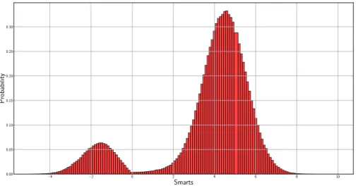
In this section, we present the results of some numerical simulations. In Subsection 4.1, we provide some histograms of the density. In Subsection 4.2, we take profit from the knowledge of the distribution function of the position of the Skew Brownian motion to perform finer tests that show a good accuracy.
4.1 Numerical approximations of the densities
4.1.1 Histograms for Skew Brownian Motion SBM (case 𝛾+= 𝛾− = 0)
First let us consider some experiments with the Skew Brownian Motion (SBM) which is a
DSBM with zero drift (case 𝛾+= 𝛾− = 0). In Figures 1 and 2, we compare the histogram
obtained with the GEARED algorithm to the true density whose formula can be found e.g. in [30,42]. −4 −2 0 2 4 Smarts 0.0 0.1 0.2 0.3 0.4 0.5 Probabilit y
Figure 1: Histogram obtained with the GEARED algorithm using 250 000 samples of a SBM with parameters 𝜃 = 2𝛽 − 1 = 0.4 (𝛽 = 0.7), 𝑥 = 0 , 𝑇 = 1.0, ∆𝑡 = 𝑇 /𝑛 and 𝑛 = 500. Comparison with the true density (solid line).
−4 −2 0 2 4 Smarts 0.0 0.1 0.2 0.3 0.4 0.5 Probabilit y
Figure 2: Histogram obtained with the GEARED algorithm using 250 000 samples of a SBM with parameters 𝜃 = 2𝛽 − 1 = −0.4 (𝛽 = 0.3), 𝑥 = 0 , 𝑇 = 1.0, ∆𝑡 = 𝑇 /𝑛 and 𝑛 = 500. Comparison with the true density (solid line).
4.1.2 Histograms for DSBM
In Figures 3 and 4, the density of the DSBM for several values of 𝛾− = 𝛾+ is given. Various
situations could be obtained that show that the Gaussian approximation is not suitable. The density could even be bimodal in some situations. Explicit formula for the density could be found in [3,16,28]. −6 −4 −2 0 2 Smarts 0.00 0.05 0.10 0.15 0.20 0.25 0.30 0.35 Probabilit y
Figure 3: Histogram obtained with the GEARED algorithm using 250 000 samples of a
DSBM with parameters 𝜃 = 2𝛽 − 1 = 0.5 (𝛽 = 0.75), 𝛾− = 𝛾+ = −2.0, 𝑥 = 0 , 𝑇 = 1.0,
∆𝑡 = 𝑇 /𝑛and 𝑛 = 500. Comparison with the true density (solid line).
−2 0 2 4 6 Smarts 0.00 0.05 0.10 0.15 0.20 0.25 0.30 0.35 0.40 Probabilit y
Figure 4: Histogram obtained with the GEARED algorithm using 250 000 samples of a
DSBM with the parameters 𝜃 = 2𝛽 − 1 = 0.5 (𝛽 = 0.75), 𝛾−= 𝛾+ = 2.0, 𝑥 = 0 , 𝑇 = 1.0,
4.1.3 Densities of some very irregular DSBM
In Figures 5 and 6, the density of the DSBM for several values of 𝛾− and 𝛾+ is represented.
No explicit formula is known for the density although an explicit expression is known for the resolvent [28]. The non-Gaussian character is obvious.
−4 −2 0 2 4 6 8 10 Smarts 0.00 0.05 0.10 0.15 0.20 0.25 0.30 Probabilit y
Figure 5: Histogram obtained obtained with the GEARED algorithm using 1 000 000 samples
of a DSBM with the parameters 𝜃 = 2𝛽 − 1 = 0.25 (𝛽 = 0.625), 𝛾− = −1.0, 𝛾+ = 4.5,
𝑥 = 0 , 𝑇 = 1.0, ∆𝑡 = 𝑇 /𝑛 and 𝑛 = 500. −2 0 2 4 6 8 10 Smarts 0.00 0.05 0.10 0.15 0.20 0.25 0.30 0.35 0.40 Probabilit y
Figure 6: Histogram obtained with the GEARED algorithm using 1 000 000 samples of a
DSBM with the parameters 𝜃 = 2𝛽 − 1 = 0.35 (𝛽 = 0.675), 𝛾− = 2.0, 𝛾+ = 5.0, 𝑥 = 0 ,
4.2 Convergence and reliability
We present in this subsection some further numerical results to assess the quality of the GEARED algorithm.
4.2.1 Kolmogorov-Smirnov test
The Kolmogorov-Smirnov test allows one to test if an empirical distribution function follows a theoretical one. We use it to test whether or not the empirical density given by the scheme is close enough to the real one.
Unlike some particular cases discussed in [28], we have no tractable analytic expression of the density or the distribution of the marginal distribution of the DSBM in general
when 𝛾+ or 𝛾− do not vanish. As a result, we consider only the case of a SBM 𝑋 with
a parameter 𝜃 = 2𝛽 − 1 whose distribution function can easily be computed from the
explicit expression of the density of the SBM (that is when 𝛾+ = 𝛾−= 0) [30,42]
𝐹𝑇(𝑥) = P[𝑋𝑇 ≤ 𝑥] = {︃ 𝑃 (𝑥 − 𝑥0, 𝑡) − 𝜃𝑃 (𝑥 − |𝑥0|, 𝑡) if 𝑥 < 0, 𝑃 (𝑥 − 𝑥0, 𝑡) + 𝜃(𝑃 (𝑥 + |𝑥0|, 𝑡) − 𝑃 (−|𝑥0|, 𝑡) if 𝑥 ≥ 0 with 𝑃 (𝑥, 𝑡) = √1 2𝜋𝑡 ∫︁ 𝑥 −∞ exp(︂−𝑦 2 2𝑡 )︂ d𝑦. Let us denote by 𝑋(𝑛,𝑖)
𝑇 the position of the 𝑖-th particle at time 𝑇 with 𝑁 independent
samples after 𝑛 steps when the starting point is 𝑥0. Thanks to Proposition 2.3, the
distribution of 𝑋(𝑛,𝑖)
𝑇 is close to the one of 𝑋𝑇. This implies that the empirical distribution
function of {𝑋(𝑛,𝑖) 𝑇 }𝑖=1,...,𝑁 𝐹𝑇(𝑛,1:𝑁 )(𝑥) = 1 𝑁 𝑁 ∑︁ 𝑖=1 1𝑋(𝑛,) 𝑇 ≤𝑥 , 𝑥 ∈ R,
is close to the distribution function 𝐹𝑇(𝑥) = P[𝑋𝑇 ≤ 𝑥] of 𝑋𝑇 with 𝑋0 = 𝑥.
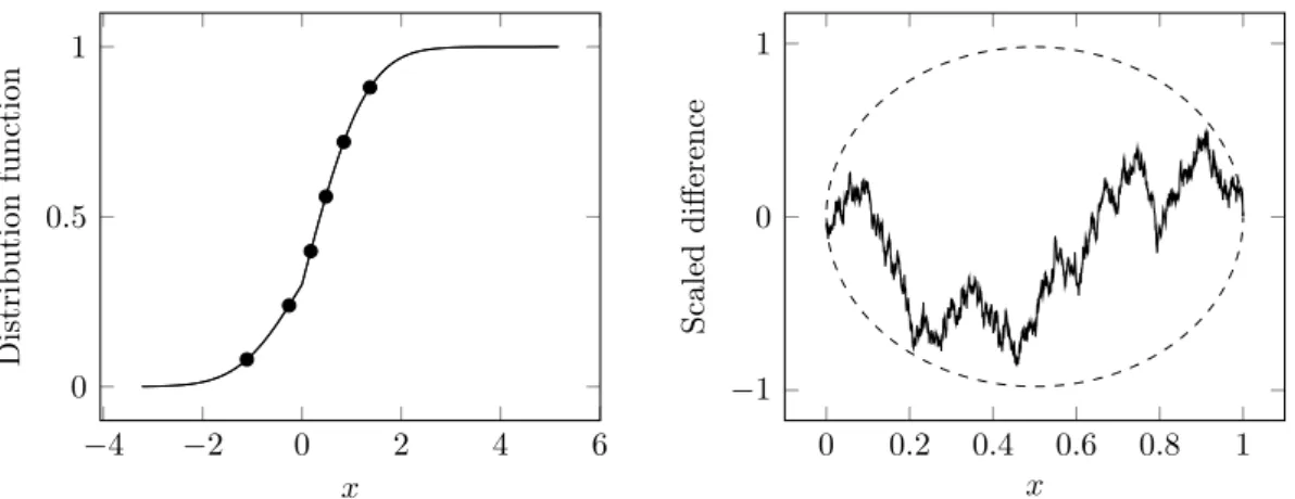
In Figure 7, we plot the difference between 𝐹(𝑛,1:𝑁 )
𝑇 and 𝐹𝑇 on the left. Let {𝑋
(𝑖)
𝑇 }𝑖=1,...,𝑁
be 𝑁 independent samples of 𝑋𝑇.
Owing to the properties of the distribution functions, {𝐹𝑇(𝑋
(𝑖)
𝑇 )}𝑖=1,...,𝑁 is distributed like
{𝑈𝑖}
𝑖=1,...,𝑁 for 𝑁 independent samples of the uniform distribution over [0, 1]. If we denote
by 𝐺(𝑁 )
𝑇 the empirical distribution function of {𝑈𝑖}𝑖=1,...,𝑁, then 𝑥 ↦→
√
𝑁 (𝐺(𝑁 )𝑇 (𝑥) − 𝑥)
converges as 𝑁 tends to infinity to a Brownian bridge. Therefore, for each 𝑥 ∈ [0, 1], √
𝑁 (𝐺(𝑁 )𝑇 (𝑥) − 𝑥)looks like a Gaussian random variable with mean 0 and variance 𝑥(1−𝑥).
A confidence band can thus be constructed this way.
The empirical distribution function of {𝐹𝑇(𝑋
(𝑛,𝑖) 𝑇 )}𝑖=1,...,𝑁 is 𝐹 (𝑛,1:𝑁 ) 𝑇 ∘ 𝐹 −1 𝑇 .
In Figure 7, we represent the scaled difference 𝐷𝑛,1:𝑁 : 𝑥 ∈ [0, 1] ↦→
√
𝑁 ((𝐹𝑇(𝑛,1:𝑁 )) ∘
𝐹−1(𝑥) − 𝑥). The more this difference looks like a Brownian bridge 𝐵br, the more accurate
is the scheme. We see that after 100 steps, the scaled difference given by the sample cannot be distinguished from a Brownian bridge.
−4 −2 0 2 4 6 0 0.5 1 x Distribution function 0 0.2 0.4 0.6 0.8 1 −1 0 1 x Scaled difference
Figure 7: Left: The empirical distribution function 𝐹(𝑛,1:𝑁 )
𝑇 of the positions {𝑋
(𝑛,𝑖)
𝑇 }𝑖=1,...,𝑛
of the scheme after 𝑛 steps (solid line) against the true distribution function (dots) using
𝑁 samples. Right: Scaled difference 𝐷𝑛,1:𝑁 : 𝑥 ∈ [0, 1] ↦→
√
𝑁 ((𝐹𝑇(𝑛,1:𝑁 )) ∘ 𝐹 (𝑥) − 𝑥) and
95 %-confidence bands given by 𝑥 ↦→ ±1.95√︀𝑥(1 − 𝑥). Parameters: 𝜃 = 2𝛽 − 1 = 0.4,
𝛾+ = 𝛾−= 0, 𝑇 = 1, 𝑋0 = 0, 𝑁 = 250 000 (number of particles) and 𝑛 = 100 (number of
steps).
The Kolmogorov-Smirnov statistics is the maximum of the absolute value of the scaled
difference |𝐷𝑛,1:𝑁(𝑥)|for 𝑥 ∈ [0, 1]. This statistics i compared with the maximum of the
Brownian bridge. In Table 1, we give the value of 𝑑 = max𝑥∈[0,1]|𝐷𝑛,1:𝑁(𝑥)| in function of
the number of steps 𝑛, as well as the 𝑝-value P[max|𝐵br| > 𝑑] for a Brownian bridge 𝐵br.
This shows the good agreement of the distribution functions, even for only 100 steps.
4.3 Repartition of mass
As shown in [31], it seems to be crucial for the accuracy of the GEARED algorithm that the proportion of particles in a given zone (distribution of mass) is as accurate as possible, especially for application towards physics.
From its very construction, the mass on each side of the interface is preserved. We now
consider the mass in a narrower zone 𝐽, which is nothing more than 𝑚𝑛
𝐽 = P[𝑋
(𝑛,1)
𝑇 ∈ 𝐽].
The latter quantity is approximated by 𝑚𝑛,1:𝑁
𝐽 =
1 𝑁
∑︀𝑁
𝑖=11𝑋(𝑛,𝑖)𝑇 ∈𝐽. In Figure 8, we plot
the estimation of the mass as well as confidence intervals constructed from Binomial distributions. Again, we find very good agreements even for only 100 steps.
4.4 Comparison between the Monte Carlo approximation and
an approximated one
At last, for the DSBM, we compare the exact density computed through a numerical inversion of the Laplace transform with the one of the scheme given by composing the resolvent kernel 𝑛 times as in (2.4). The later quantity is computed by discretizing the integrals. Even for a small number of steps (𝑛 = 30), we see in Figure 9 that the density of the scheme converges quickly to the true density, even when the latter is discontinuous at 0.
𝑛 distance 𝑑 𝑝-value distance 𝑑 𝑝-value 𝜃 = 0.4 𝜃 = −0.2 100 0.0017 0.44 0.0023 0.13 150 0.0017 0.48 0.0028 0.04 200 0.0017 0.49 0.0016 0.58 250 0.0013 0.82 0.0018 0.42 300 0.0024 0.10 0.0015 0.64 350 0.0015 0.59 0.0013 0.76 400 0.0019 0.34 0.0020 0.26 450 0.0012 0.86 0.0028 0.05 500 0.0018 0.40 0.0018 0.40
Table 1: Kolmogorov-Smirnov statistics in function of the number 𝑛 of steps. Parameters:
𝜃 = 2𝛽 − 1 ∈ {0.4, −0.2}, 𝛾+ = 𝛾− = 0, 𝑇 = 1, 𝑋0 = 0, 𝑁 = 250 000 (number of particles)
𝑋0 = 0 and 𝑛 is the number of steps.
200 400 0.95 0.95 0.95 0.96 steps n Mass m [− 2 ,2] 200 400 0.7 0.7 0.7 steps n Mass m [0 ,+ ∞ ) 200 400 0.95 0.95 0.95 steps n Mass m [0 ,+ ∞ ) 200 400 0.4 0.4 0.4 steps n Mass m [0 ,+ ∞ ) (a) θ = 0.7 (b) θ = −0.2
Figure 8: Estimation of the empirical probabilities 𝑚𝑛,1:𝑁
𝐽 for 𝐽 = [−2, 2] and 𝐽 = [0, +∞)
as a function of the number of steps 𝑛 (solid), with a 95 %-confidence interval, and comparison with the true value (horizontal line). Parameters: 𝜃 = 2𝛽 − 1 ∈ {0.7, −0.2},
𝛾+ = 𝛾−= 0, 𝑇 = 1, 𝑋0 = 0, 𝑁 = 250 000 (number of particles) and 𝑛 ∈ 100, 150, . . . , 500
−6 −4 −2 0 2 4 6 0.0 0.1 0.2 0.3 0.4
Figure 9: Exact density obtained by numerical Laplace inversion of the resolvent (solid) and density of the scheme obtained by composition the resolvent kernel 𝑛 times (dashed).
Parameters: 𝜃 = 2𝛽 − 1 = 0.5, 𝛾+ = 𝛾− = 1, 𝑇 = 1, 𝑋0 = 0, and 𝑛 = 30 (number of
steps).
5 Conclusion
Often close form analytic expressions of the resolvent kernel of diffusion processes are easier to obtain than close form analytic expressions of the density. In that cases, the GEARED algorithm offers a very interesting alternative to simulate diffusion processes in media with discontinuous coefficients. We applied this algorithm to the case of piecewise constant coefficients since, in that case, the resolvent kernel has a simple and tractable expression. Numerical simulations showed a good fit of the simulated densities, a correct repartition of mass and a fast convergence to the true density. We are currently investigating the use of this algorithm in dimensions greater than 1 and in the case of diffusion of other nature.
Acknowledgments. This work was supported by ANR-MN, with the H2MNO4 project (Projet-ANR-12-MONU-0012).
References
[1] H. Alzubaidi. Random timestepping algorithm with exponential distribution for pricing various structures of one-sided barrier options. American Journal of Computational
Mathematics, 7(3):228–242, 2017.
[2] Hasan Alzubaidi and Tony Shardlow. Improved simulation techniques for first exit time of neural diffusion models. Comm. Statist. Simulation Comput., 43(10):2508–2520, 2014.
[3] T. Appuhamillage, V. Bokil, E. Thomann, E. Waymire, and B. Wood. Occupation and local times for skew Brownian motion with applications to dispersion across an interface. Ann. Appl. Probab., 21(5):2050–2051, 2011.
[4] Anthony Beaudoin and Jean-Raynald De Dreuzy. Numerical assessment of 3-D
macrodispersion in heterogeneous porous media. Water Resources Research,
[5] M. Bechtold, J. Vanderborght, O. Ippisch, and H.V. Vereecken. Efficient random walk particle tracking algorithm for advective-dispersive transport in media with discon-tinuous dispersion coefficients and water contents. Water Resour. Res.,, 47:W10526, 2011.
[6] P. Billingsley. Convergence of Probability Measures. Wiley series in probability and statistics. Wiley-Interscience publication, 2 edition, 1999.
[7] M. Bossy, N. Champagnat, S. Maire, and D. Talay. Probabilistic interpretation and random walk on spheres algorithms for the Poisson-Boltzmann equation in molecular dynamics. M2AN Math. Model. Numer. Anal., 44(5):997–1048, 2010.
[8] R.S. Cantrell and C. Cosner. Diffusion models for population dynamics incorporat-ing individual behavior at boundaries: Applications to refuge design. Theoretical
Population Biology, 55(2):189–207, 1999.
[9] Kai lai Chung. On the exponential formulas of semi-group theory. Math. Scand, 10:153–162, 1962.
[10] M. Decamps, A. De Schepper, and M. Goovaerts. Applications of 𝛿-function pertur-bation to the pricing of derivative securities. Phys. A, 342(3-4):677–692, 2004. [11] F. Delay, Ph. Ackerer, and C. Danquigny. Simulating solute transport in porous or
fractured formations using random walks particle tracking: A review. Vadose Zone
J., 4:360–379, 2005.
[12] D. Dereudre, S. Mazzonetto, and S. Roelly. An explicit representation of the transition densities of the skew Brownian motion with drift and two semipermeable barriers. http://arxiv.org/abs/1509.02846v1, 2015.
[13] L. Devroye. Non-Uniform Random Variate Generation. Springer-Verlag, 1986. [14] P. Étoré. On random walk simulation of one-dimensional diffusion processes with
discontinuous coefficients. Electron. J. Probab., 11:no. 9, 249–275 (electronic), 2006. [15] P. Étoré and A. Lejay. A Donsker theorem to simulate one-dimensional processes
with measurable coefficients. ESAIM Probab. Stat., 11:301–326, 2007.
[16] P. Étoré and M. Martinez. Exact simulation of one-dimensional stochastic differential equations involving the local time at zero of the unknown process. Monte Carlo
Methods and Applications, 19(1):41–71, 2013.
[17] A. Gairat and V. Shcherbakov. Density of skew Brownian motion and its functionals with application in finance. Mathematical Finance, 26(4):1069–1088, 2016.
[18] H. Hoteit, R. Mose, A. Younes, F. Lehmann, and Ph. Ackerer. Three-dimensional modeling of mass transfer in porous media using the mixed hybrid finite elements and the random-walk methods. Mathematical Geology, 34(4):435–456, 2002.
[19] K. Itô and H. P. McKean. Diffusion processes and their sample paths. Springer-Verlag, 2 edition, 1974.
[20] S. Janson. Tail bounds for sums of geometric and exponential variables. Statistics &
[21] K. M. Jansons and G. D. Lythe. Efficient numerical solution of stochastic differential equations using exponential timestepping. J. Statist. Phys., 100(5-6):1097–1109, 2000. [22] K. M. Jansons and G. D. Lythe. Exponential timestepping with boundary test for
stochastic differential equations. SIAM J. Sci. Comput., 24(5):1809–1822, 2003. [23] K. M. Jansons and G. D. Lythe. Multidimensional exponential timestepping with
boundary test. SIAM J. Sci. Comput., 27(3):793–808, 2005.
[24] P. E. Kloeden and E. Platen. Numerical Solution of Stochastic Differential Equations, volume 23 of Stochastic Modelling and Applied Probability. Springer-Verlag Berlin Heidelberg, 1992.
[25] E. M. LaBolle, G. E. Fogg, and A. F. B. Tompson. Random-walk simulation of transport in heterogeneous porous media: Local mass-conservation problem and implementation methods. Water Resources Research, 32(3):583–593, 1996.
[26] E. M. LaBolle, Quaster J., and G. E. Fogg. Diffusion theory for transport in porous media: Transition‐probability densities of diffusion processes corresponding to advection‐dispersion equations. Water Resources Research, 34(7):1685–1693, 1998. [27] J. Langebrake, L. Riotte-Lambert, C. W. Osenberg, and P. De Leenheer.
Differen-tial movement and movement bias models for marine protected areas. Journal of
Mathematical Biology, 64(4):667–696, 2012.
[28] A. Lejay, L. Lenôtre, and G. Pichot. Analytic expressions of the solutions of advection-diffusion problems in 1d with discontinuous coefficients, 2017.
[29] A. Lejay and M. Martinez. A scheme for simulating one-dimensional diffusion processes with discontinuous coefficients. Ann. Appl. Probab., 16(1):107–139, 02 2006.
[30] A. Lejay and G. Pichot. Simulating diffusion processes in discontinuous media: A numerical scheme with constant time steps. Journal of Computational Physics, 231(21):7299 – 7314, 2012.
[31] A. Lejay and G. Pichot. Simulating diffusion processes in discontinuous media: benchmark tests. J. Comput. Phys., 314:384–413, 2016.
[32] H. P. McKean, Jr. Elementary solutions for certain parabolic partial differential equations. Trans. Amer. Math. Soc., 82:519–548, 1956.
[33] B. Noetinger, D. R. Roubinet, J. R. De Dreuzy, A. R. Russian, P. Gouze, T. Le Borgne, M. Dentz, and F. Delay. Random walk methods for modeling hydrodynamic transport in porous and fractured media from pore to reservoir scale. Transport in Porous
Media, 115(2):345 – 385, 2016.
[34] A. Pazy. Semigroups of linear operators and applications to partial differential
equations, volume 4 of Applied Mathematical Sciences. Springer, 1983.
[35] W. Peter. Quiet direct simulation Monte-Carlo with random timesteps. J. Comput.
Phys., 221(1):1–8, 2007.
[36] J. Pitman and M. Yor. Hitting, occupation and inverse local times of one-dimensional diffusions: martingale and excursion approaches. Bernoulli, 9(1):1–24, 2003.
[37] J. M. Ramirez, E. A. Thomann, E. C. Waymire, J. Chastanet, and B. D. Wood. A note on the theoretical foundations of particle tracking methods in heterogeneous porous media. Water Resources Research, 44(1):n/a–n/a, 2008. W01501.
[38] P. Salamon, D. Fernàndez-Garcia, and J. J. Gómez-Hernández. A review and numerical assessment of the random walk particle tracking method. J. Contaminant Hydrology, 87(3-4):277–305, 2006.
[39] D. Spivakovskaya, A. W. Heemink, and E. Deleersnijder. Lagrangian modelling of multi-dimensional advection-diffusion with space-varying diffusivities: theory and idealized test cases. Ocean Dynamics, 57(3):189–203, 2007.
[40] D.J. Thomson, W.L. Physick, and R.H. Maryon. Treatment of interfaces in random walk dispersion models. Journal of Applied Meteorology, 36:1284–1295, 1997.
[41] G.J.M. Uffink. A random walk method for the simulation of macrodispersion in a stratified aquifer. Relation of Groundwater Quantity and Quality, IAHS Publication, 146:103–114, 1985.
[42] J. B. Walsh. A diffusion with discontinuous local time. In Temps locaux, volume 52-53, pages 37–45. Société Mathématique de France, 1978.
[43] S. Wang, S. Song, and Y. Wang. Skew Ornstein-Uhlenbeck processes and their financial applications. J. Comput. Appl. Math., 273:363–382, 2015.
[44] M. Zhang. Calculation of diffusive shock acceleration of charged particles by skew Brownian motion. The Astrophysical Journal, 541:428–435, 2000.
[45] C. Zheng and G. D. Bennett. Applied Contaminant Transport Modelling. Wiley-Interscience, second edition, 2002.