HAL Id: hal-01030845
https://hal.inria.fr/hal-01030845
Submitted on 22 Jul 2014
HAL is a multi-disciplinary open access
archive for the deposit and dissemination of
sci-entific research documents, whether they are
pub-lished or not. The documents may come from
teaching and research institutions in France or
abroad, or from public or private research centers.
L’archive ouverte pluridisciplinaire HAL, est
destinée au dépôt et à la diffusion de documents
scientifiques de niveau recherche, publiés ou non,
émanant des établissements d’enseignement et de
recherche français ou étrangers, des laboratoires
publics ou privés.
A Surface Reconstruction Method for In-Detail
Underwater 3D Optical Mapping
Ricard Campos, Rafael Garcia, Pierre Alliez, Mariette Yvinec
To cite this version:
Ricard Campos, Rafael Garcia, Pierre Alliez, Mariette Yvinec. A Surface Reconstruction Method for
In-Detail Underwater 3D Optical Mapping. The International Journal of Robotics Research, SAGE
Publications, 2015, 34 (1), pp.25. �10.1177/0278364914544531�. �hal-01030845�
A Surface Reconstruction Method for In-Detail Underwater 3D
Optical Mapping
Ricard Campos, Rafael Garcia
Computer Vision and Robotics Group University of Girona, Spain
[email protected], [email protected]
Pierre Alliez
Titane
INRIA Sophia Antipolis - M´editerran´ee, France [email protected]
Mariette Yvinec
Geometrica
INRIA Sophia Antipolis - M´editerran´ee, France [email protected]
Abstract
Underwater range scanning techniques are starting to gain interest in underwater exploration, provid-ing new tools to represent the seafloor. These scans (often) acquired by underwater robots usually result in an unstructured point cloud, but given the common downward-looking or forward-looking configura-tion of these sensors with respect to the scene, the problem of recovering a piecewise linear approximaconfigura-tion representing the scene is normally solved by approximating these 3D points using a heightmap (2.5D). Nevertheless, this representation is not able to correctly represent complex structures, especially those presenting arbitrary concavities normally exhibited in underwater objects. We present a method devoted to full 3D surface reconstruction that does not assume any specific sensor configuration. The method presented is robust to common defects in raw scanned data such as outliers and noise often present in extreme environments such as underwater, both for sonar and optical surveys. Moreover, the proposed method does not need a manual preprocessing step. It is also generic as it does not need any information other than the points themselves to work. This property leads to its wide application to any kind of range scanning technologies and we demonstrate its versatility by using it on synthetic data, controlled laser-scans, and multibeam sonar surveys. Finally, and given the unbeatable level of detail that optical methods can provide, we analyze the application of this method on optical datasets related to biology, geology and archeology.
1
Introduction
Unmanned sea exploration using autonomous robots has undergone important improvements in recent years, proving to be very useful in collecting data at depths otherwise unreachable by humans. These robots are equipped with sensors to gather the required information for navigation (DVL, USBL, IMU, ...) and also for mapping purposes. Within this sensor suite, cameras are an important and low-cost component, and while they can be used in some cases to aid navigation (Elibol et al., 2013), they are mostly used for mapping (Singh et al., 2007).
Although underwater imaging is an important tool to understand the many geological and biological processes taking place on the seafloor, phenomena such as light attenuation, blurring, low contrast or variable illumination (normally caused by the required artificial lighting) makes optical surveying a difficult task underwater. Despite these limitations, images provide data that is easily interpretable by humans, and thus their importance in underwater exploration is indisputable (Gracias et al., 2013).
On the other hand, it is important to provide all the data collected by the submersibles in a way that is easily understandable by the experts who will work with it. Among others, biologists, geologists and archeologists need to extract conclusions based on the acquired data. However, the vast amount of data gathered during a mission makes interpretation quite confusing. Take, for instance, the case of optical sensors, which are systematically present in most underwater vehicles. Due to the phenomena presented above, which make underwater imaging extremely noisy, these robots must dive to within a very close range
to the area being surveyed to obtain faithful images, which causes the information in a single image to be very local. For this reason, these individual images are often gathered together in some way to provide a global view of the observed zone. Photomosaics, for example, have been very useful in describing large underwater areas (Barreyre et al., 2012). This kind of representation assumes that the robot has been observing the area from a downward-looking camera with its optical axis almost perpendicular to the seafloor (e.g., Ferrer et al. (2007)). Although this is useful, this representation assumes the observed scene to be almost planar, which is not the case when 3D structures are present (see Nicosevici et al. (2009)). Thus, a better approximation for areas with 3D relief is needed.
Underwater 3D mapping has normally been carried out by acoustic multibeam sensors. Note however that the information provided by multibeam or sidescan sonars is normally gathered in the form of elevation maps (i.e., 2.5D maps), which are useful for providing a rough approximation of the global shape of the area, but are not able to sense more complex structures (e.g., they cannot represent arbitrary concavities). In this kind of representation, a useful sensor fusion approach is to use the texture of a mosaic as a texture map for the triangulated height map, coupling in this way the small details captured by the camera with the rough elevation map provided by the multibeam sonar. However, these 2.5D representations are normally approximations of the true 3D geometry of the area. In this article we focus on using the imaging information alone to provide a high quality representation of small areas of interest in high resolution.
As mentioned above, typical underwater optical mapping has been carried out using cameras that are orthogonal to the seafloor. However, in this article we go for a more general scenario, where the camera can be mounted in a general configuration; that is, located anywhere on the robot and with any orientation. With this new configuration, objects can be observed from new viewpoints. Viewing the object from arbitrary positions allows a better understanding of the global shape of the object since its features can be observed from angles that are more suitable to their exploration. Take as example the trajectory in Figure 1, corresponding to a survey of an underwater hydrothermal vent (further results with this dataset are illustrated in Section 7). It is impossible to recover the intricate structure of this area with just a downward-looking camera. In this case, the camera was located on the front part of the robot looking approximately forward at a 75oangle with
respect to the vertical gravity vector. This configuration allowed the recovery of the many concavities this object contains. The difference in resolution and complexity of this same area when mapped using multibeam sonar technologies in a 2.5D representation are evident.
Although some underwater robots carry stereo systems, most industrial Remotely Operated Vehicles (ROVs) nowadays incorporate a single video camera, often not synchronized to its navigation readings. Even in this case, and using monocular video readings, the image-based 3D reconstruction can be solved. This problem has been studied extensively in the computer vision community. The common pipeline starts by calibrating the intrinsic parameters of the camera (Bouguet, 2003) in order to obtain a geometric model of a pinhole camera that allows further computations to be performed. Next, both the structure in the scene and the camera trajectory are recovered using a structure-from-motion procedure based on matching relevant image features from a number of images. In our case, this was implemented using the method presented by Nicosevici et al. (2009), but we changed its incremental strategy with a more global approach similar to the one presented by Snavely et al. (2006). Once the camera trajectory has been computed, the focus is put on obtaining a dense reconstruction, i.e., recovering the highest possible number of 3D points to represent the object with high fidelity. This method can follow a mostly brute force approach (Collins, 1996), where different depths are tried for each pixel to match with nearby images based on some similarity functions. From all the possible depths, the best one is selected according to some heuristics. These methods are receiving an increasing amount of attention given that they can be easily parallelizable on GPU (Yang and Pollefeys, 2003). Other methods often take advantage of the local smoothness of the surface in order to restrict the search for correspondences, as in Habbecke and Kobbelt (2007) or Furukawa and Ponce (2010). They both use a greedy approach, where the surface grows in the tangent directions of the already reconstructed points. Using a monocular moving camera, and without assuming any other information being provided to the system, the recovered reconstructions are always affected by an unknown scale factor (Hartley and Zisserman, 2004). This scale factor needs to be recovered in order to provide a metric reconstruction. Of course, having a metric reconstruction would allow the reconstructed model to be not just useful for visualization purposes, but also for taking measurements from it. This can be accomplished by enforcing some real-world constraints, such as the knowledge of some world measures or relating some external metric sensor measures to the images, as proposed in Garcia et al. (2011).
Up to this point, the scene is only described in the form of a noisy point cloud containing a large number of outliers due to the nature of the underwater medium. Unfortunately, this representation is not enough
(a)
(b)
Figure 1: (a) Example of a more general trajectory, with a frame representing each camera. This is the trajectory used for mapping the Tour Eiffel hydrothermal chimney at a depth of about 1700 meters in the Mid-Atlantic ridge. In this case, the camera was pointing towards the object, in a forward-looking configuration. The shape of the object shown was recovered using our approach. Note the difference in the level of detail when compared with a 2.5D representation of the same area obtained using a multibeam sonar in (b). The trajectory followed in (b) was a downward-looking hovering over the object. The trajectory in (b), shown in blue, corresponds to the survey in (a).
for further processing of the data. Besides, proper visualization of the data is not possible, since point sets lack visibility information, which means that, for a given viewpoint, the viewer may not be able to tell which points should be visible and which should be occluded. Take, as example, any of the results shown in Section 7, where the plotting of the point cloud alone provides little information on the shape of the object when projected onto the figure. In the case of classic multibeam sonar imagery, this 2.5D point cloud is triangulated on the plane using a regular grid or, alternatively, a planar triangulation such as Delaunay. However, in the case of full 3D geometry the problem becomes ill-posed.
We aim at recovering the shape of the object from the set of points describing it while, at the same time, getting rid of the outliers, improving data visualization. This is referred to in the literature as the surface reconstruction problem, and has been extensively studied in recent years by many research areas, including computational geometry, computer graphics and computer vision. The problem consists of finding a surface mesh (normally with triangles as primitives) that interpolates or approximates the input points. Note that for a given point cloud, one can propose many surfaces that pass over or near the points. For this reason, the problem relies on finding the most probable surface based on the sampling that the points represent. Furthermore, we have to take into account that point sets coming from real-world datasets are often not ideal as they are normally corrupted by both noise and outliers (Rousseeuw and Leroy, 1987). Noise refers to the quality of the measurement and are variations caused by the precision or repeatability of the reconstruction method, or the quality of the reconstructed point. Outliers are totally wrong or spurious measurements, that is, they do not represent a sample of the surface, and are normally caused by errors during the point set recovery process.
In this paper, we present a novel method for surface reconstruction able to provide a smooth surface approximation from a point set. This method can handle noise and cope with a large percentage of outliers, which is often the case for underwater datasets. Moreover, additional information such as per-point normals or local connectivity is not required. Despite the fact that the procedure is focused on applying this method to point sets coming from a computer vision pipeline, it is worth noticing that its generality makes it applicable to all kinds of point set data. For instance, we report results of applying the method to a multibeam sonar dataset acquired by an underwater robot while surveying an underwater 3D structure; the different scans are registered into a common frame, and then this data is used as input for our method. It should be noted that when a robot is exploring a 3D scene, going from a cloud of 3D points to a meshed surface is the first step towards space awareness, and this becomes even more relevant if the scene is cluttered and the point set noisy.
Our method is inspired by the Restricted Delaunay Triangulation (RDT) meshing paradigm. As will be presented in the following sections, the RDT meshing method starts from a small set of points and iteratively constructs a triangle surface following a coarse-to-fine procedure. The method is quite generic, as it only requires the ability to answer line segment intersection queries on the surface to be meshed. Thus, what we propose is to answer these queries on-line, by constructing a local surface in a neighborhood around the query segment, and returning the intersection of this local surface with the query segment. The method takes into account possible aberrations in the data by using RANSAC in order to recover the local surface with the highest support. Furthermore, noise is not considered constant, and an automatic scale computation algorithm is used in order to guess the best RANSAC distance-to-model threshold to apply at each step. The main advantage of using the mesher algorithm as a base is to be able to tune the desired resolution of the resulting surface, a parametrization that is not available in most of the state-of-the-art approaches. Besides, our method also provides the ability to recover surfaces with boundaries. This is desirable in an underwater scenario, where a part of the seafloor is normally observed, and thus the retrieved point set does not represent a watertight surface.
When compared to methods in the state of the art, our proposal has the advantage of being able to process highly corrupted point sets without additional information. The loose requirements for the input, and its low memory footprint, make this method suitable for completing the modelling pipeline in the complex underwater environment.
2
Related Work
We divide the previous work related to this paper into two main sections. First, we review the methods used to recover 3D underwater structures, as this is our main application area. Then, we survey the solutions proposed for the surface reconstruction problem, with various methods that can be applied to arbitrary point
cloud datasets, regardless of the application area. Furthermore, in each section we describe the contributions our proposed method provides.
2.1
Underwater Optical 3D Mapping
As previously stated, underwater mapping relies primarily on assuming an underlying planar structure, common throughout the survey, where a 2.5D representation of the shape can be built. The problem of large area mapping is often tackled by using downward-looking cameras/sensors, since their overview capabilities provides an overall notion of the shape of the scene. The use of this approximation has motivated the widely spread use of scanning sensors located at the bottom of the vehicles, with their optical axis orthogonal to the seafloor.
There is a great deal of literature on the different uses of this scanning configuration for sonar mapping. Automatic methods to build these maps out of raw sonar readings has been a hot research topic in recent years (Roman and Singh, 2007; Barkby et al., 2012). The application of these techniques has proven to provide key benefits for other research areas such as archeology (Bingham et al., 2010) or geology (Yoerger et al., 2000), to name a couple. Given the depth readings, retrieving a surface representation is straightforward. By defining a common plane, all the measures can be projected in 2D. Then, an irregular triangulation like Delaunay or a gridding technique can be applied to the projections on the plane and the 3rd coordinate is used to lift the surface in a 2.5D representation. These mappings can be enhanced by using photomosaics as texture, thus producing a multimodal representation of the area (Johnson-Roberson et al., 2009).
On the other hand, although not that extensive, cameras are also used for heightmap reconstruction. Regarding full 3D reconstruction, the methods in the literature are more concerned with recovering the point set, obviating the surface reconstruction part. Thus, the focus is normally put on the registration of multiple camera positions, using either structure-from-motion systems (Nicosevici et al., 2009; Bryson et al., 2012) or simultaneous localization and mapping approaches (Johnson-Roberson et al., 2010) using monocular or stereo cameras (Mahon et al., 2011). As previously stated, the common downward-looking camera configuration makes methods tend to represent the shape underlying these points as a heightmap in a common reference plane, which may be easily extracted using Principal Component Analysis (PCA) (Singh et al., 2007; Nicosevici et al., 2009).
There are very few proposals on underwater mapping using some of the existing surface reconstruction techniques. In Johnson-Roberson et al. (2010), the authors do use a volumetric method from Curless and Levoy (1996), originally devised to full 3D reconstruction. Nevertheless, the camera is still observing the scene in a downward-looking configuration, and the added value of applying this method in front of a 2.5D approximation is not discussed. Nonetheless, they establish an approach to parallelize the reconstruction using this method on small chunks of data at a time and then merging the results. Another proposal, this time using a forward-looking camera and working on a more complex structure, is the one presented in Garcia et al. (2011), where an underwater hydrothermal vent is reconstructed using dense 3D point cloud retrieval techniques and the Poisson surface reconstruction method (Kazhdan et al., 2006).
The review of the state of the art on underwater 3D modelling has revealed that most of the proposals retrieve the surface in a 2.5D representation. Furthermore, given the straightforwardness of changing from depth readings to this representation, the creation of a triangulated elevation map is usually considered a side result. In comparison with the current approaches for 3D mapping, we aim to deal directly with the problem of surface reconstruction by giving it the relevance it deserves. The contribution of our method is to be able to represent complex 3D structures that are not representable using heightmap representations, while also providing noise correction and outlier removal.
2.2
Surface Reconstruction
Regarding the surface reconstruction problem itself, there have been mainly two types of approaches: those based on point interpolation, and those approximating the points. Normally, these kinds of methods are applied to range scan datasets, because of the spread use of these sensors nowadays. Nevertheless, they tend to be generic enough to be applicable to any point-based data regardless of their origin.
Methods trying to interpolate the points have been studied mainly by the computational geometry com-munity. They normally rely on using the input point set to define a space partition like the Delaunay triangulation. The method assumes the surface is closed and, given the space partition, the idea is to sep-arate the tetrahedrons that are part of the inside from those from the outside of the surface. Very often
they rely on theoretical proofs to reconstruct the surface when some sampling conditions have been achieved. These proofs for the ideal case are then used to define some heuristics for the practical case on real datasets, where the sampling requirements are normally not fulfilled. Two commonly known methods in this area are the Cocone method (Amenta et al., 2000), and the Power Crust method (Amenta et al., 2001). Another common approach is that of ball-pivoting (Bernardini et al., 1999), where the triangles forming the surface are incrementally constructed in a greedy manner by making local decisions on which point to insert next. Since interpolation-based methods require input points (or at least some of them) to be part of the final surface, the quality of the results is restricted by the point set fidelity according to noise. Thus, no noise correction is provided by this kind of method. However, a prior noise smoothing filter can be applied to the point set in order to improve the resulting quality of the mesh, as presented by Digne et al. (2011). Nonetheless, some interpolative methods can take into account the presence of outliers in the data. These outlier-resilient methods include the spectral graph partitioning method of Kolluri et al. (2004), or that of Labatut et al. (2007). This last one relies on the additional information of knowing the pose of the sensor at the time of capturing the scene.
On the other hand, methods based on approximation are far more varied. The vast majority of these proposals rely on defining the surface in implicit form, and then evaluating the function of each of the cells in a regular grid, discretizing the working space. The final surface triangle mesh is then extracted from this representation using a marching cubes approach (Lorensen and Cline, 1987), or one of its variants. A common approach is to define a signed distance function using the input points. Hoppe et al. (1992) proposed computing per-point normals using local neighborhoods, orienting them and using them as approximations of the tangent planes to the surface. By computing the signed distance function from each cell in the space to the closest tangent plane, they got an approximation of the distance function. In the field of range scans merging, Curless and Levoy (1996) proposed computing a signed distance field for each scan, which are easy to compute thanks to the 2D local neighborhood knowledge, and then merge the different contributions in a global signed distance function. Other approaches that also build signed distances are those using Radial Basis Functions (RBF). In this case, normals are assumed to be known in order to give the proper orientation to the distance field. However, despite their promising results, the problem resides in a single evaluation of the resulting implicit function being computationally expensive as it requires using all the points. To overcome this problem, some authors have worked in the direction of using compactly supported RBF, which do not expand throughout the whole domain, and are just affected by nearby sample points, as proposed by Ohtake et al. (2004). Using a mixed approach, the Multi-level Partition of Unity implicit method of Ohtake et al. (2003) divides the working space and computes a local quadratic fit at each subdivision, then uses RBFs for weighting the different contributions. Notice that most of the signed distance computations require the knowledge (or the heuristic computation) of normals for each input point.
Other approaches build on unsigned distance functions to work, in this way removing the need of input normals. The level sets technique proposed by Zhao et al. (2001) defines an initial surface at a given unsigned distance from the input points, and then deforms this initial approximation iteratively towards the input points. Similarly, the work presented by Hornung and Kobbelt (2006) computes the unsigned distance function in a narrow band around the points. They build a graph structure inside the regular grid discretizing the space, and then find the surface as a minimum cut inside this graph. Both methods do not assume outliers to be present in the data. The approach presented by Mullen et al. (2010) achieves robustness to outliers by computing a robust unsigned distance function. They limit themselves to working in a narrow band containing the geometry, and then try to give a coherent sign to the distance function by using some heuristics.
Finally, there are some approximation approaches where the implicit function sought is not a distance function but an indicator function. An indicator function denotes for a given point in R3 if it is part of the
interior of the object, or from the outside. Kazhdan et al. (2006) consider points with normals as samples of the vector field of the indicator function. Then, using Poisson equation, they try to solve for a function whose gradient approximates this vector field. This work has proven successful under high noise and small amounts of outliers due to its global view.
Another kind of technique that has grown in popularity in recent years is the Moving Least Squares (MLS) paradigm. This technique was first used for visualization of point clouds by Alexa et al. (2003). Given a point in space, the MLS definition provides a procedure to project the point onto the surface defined by the input point set. Moreover, most of the MLS definitions can be cast into an implicit formulation, which can be used to extract the surface in the form of a surface triangle mesh. Some of the variations proposed achieve great results in noise correction, as in the case of Algebraic Point Set Surfaces (Guennebaud and
Gross, 2007).
Normals are usually not directly available in most scanning techniques, so its requirement complicates the use of most of the methods in the state of the art. Furthermore, the problem of dealing with outliers is quite new, since many methods assume that these erroneous points have been eliminated during a preprocessing step (usually manual).
Having reviewed the state of the art in surface reconstruction, we can list the flaws detected in the above mentioned methods with respect to their application to underwater datasets, and the improvements that our method should provide. First, underwater point cloud datasets, specially (but not solely) the ones retrieved using computer vision techniques, are affected by varying noise and are normally outlier-ridden. Obviously, this is caused by the previously mentioned adverse conditions in underwater imaging. Thus, our method aims to be robust to both noise and outliers. Second, noise varies in different parts of the reconstructed surface since distance to the object, illumination conditions, etc., are not constant across images. Consequently, we aim to obtain a surface reconstruction method able to deal with varying noise values. In this direction, automatic noise scale computation methods are used in our pipeline. Most of the above described techniques impose the restriction of the object to be watertight, i.e., one can always define an inside and an outside for the surface. Note that normally this is not the case for underwater mapping, where we are usually interested in just a part of a 3D structure laying on the seafloor. Thus, the surface should be recovered just where the samples define it, and we should not extrapolate parts of the surface in places where there is no data.
3
Overview and Contributions
We base our method on the Restricted Delaunay Triangulation (RDT) meshing algorithm. This method only requires the user to provide an intersection detection between line segments and the surface in order to approximate the object with a mesh of triangles. Normally, a given approximation of the surface is devised, using for example some of the techniques described in Section 2.2, and then this approximation is meshed using RDT in order to get a surface whose triangles follow a given quality. On the contrary, what we aim to do is obtain an on-line answer to this kind of query, in this way transforming a (re)meshing method into a surface reconstruction method.
Given the query segment required by the mesher, a small local part of the surface is computed using the points falling at a given distance from it, then this local surface is tested for intersection with the segment. Our local operator works directly on the raw, and possibly corrupted, point cloud, by using robust statistic techniques in order to avoid outliers when building the small surface patch. In this sense, we use a RANSAC method whose threshold is locally adaptive to the scale of the noise in the area. Thus, when compared to the state of the art, the main contribution of our method is the ability to deal with point sets corrupted with both variable noise and outliers without any kind of additional information.
Using the surface mesher as a base provides our method with the ability of specifying the quality and properties of the resulting mesh in terms of shape and density of triangles. This allows having multiple resolutions of the same object by just tuning the parameters. Furthermore, it is worth noticing that the meshing algorithm works in a coarse to fine way, while our operator works with only a small part of the data at a time, in this way providing low memory requirements, which is the cornerstone for meshing large 3D maps.
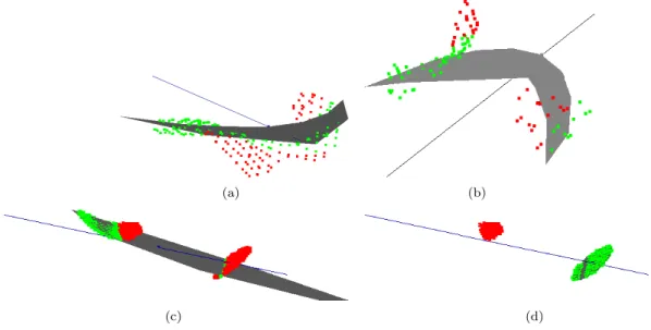
Figure 2 shows a schematic idea of our method, and in Figure 3 one can find some examples of segment queries applied to a synthetic dataset. Note how even in the presence of outliers and noise, the local procedure is able to generate a correct local surface suited to answer the intersection query.
4
Restricted Delaunay Triangulation Meshing
As stated below, the basis of our method is a surface meshing algorithm based on the concept of RDT and Delaunay refinement (Boissonnat and Oudot, 2005). Given a point set E and a surface S, the Delaunay triangulation of E restricted to S, Del|S(E), is the subcomplex of the 3D Delaunay triangulation Del(E)
formed by the facets of Del(E) whose dual Voronoi edge intersects the surface S. This concept was used to solve the surface reconstruction problem in an early paper by Amenta et al. (2001), where the authors defined the sampling E of the object required to achieve a surface reconstruction by computing this dual intersection. These sampling conditions are very difficult to fulfill on real datasets, so the aim of the RDT
(a) (b) (c)
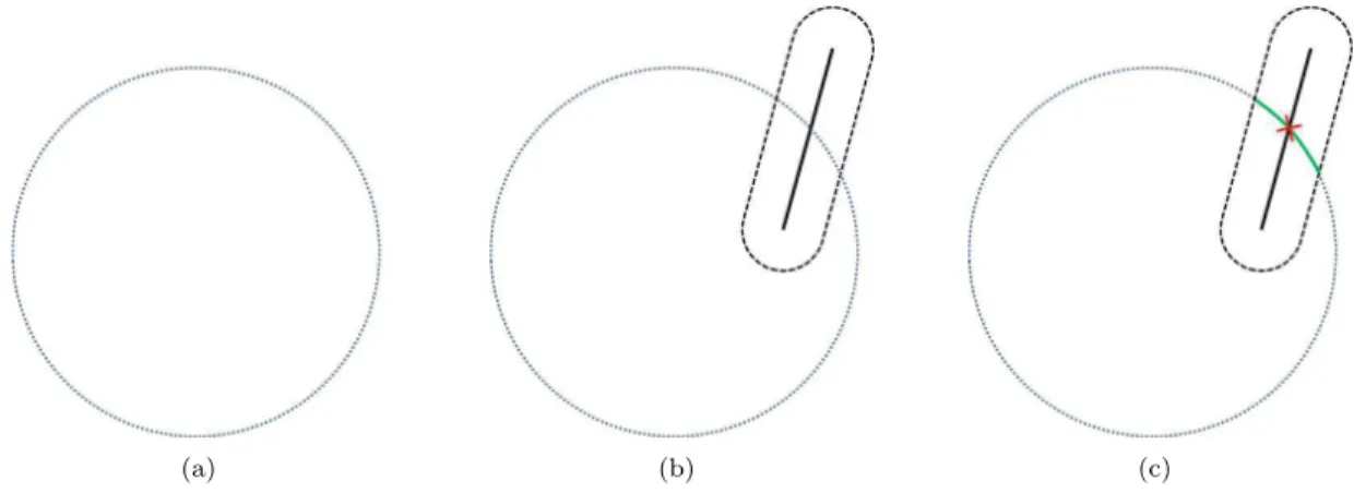
Figure 2: Schematic overview of the proposed on-line segment intersection query computation. (a) presents the input points, and (b) the query segment s and its capsule neighborhood. As depicted in (c), a local surface is fitted to the points inside the capsule neighborhood and the intersection is computed.
Figure 3: On the right are three examples of query segments required by the RDT algorithm to mesh the surface represented by the highly corrupted set of points on the left (a sphere), and the recovered local surfaces computed by our method used to solve the intersection computation. The results of our method applied to this point set can be found in Section 7.1.
meshing algorithm is to iteratively build a sample close to the ideal and, at the same time, keep track of the surface generated.
Each triangle on the RDT has a circumball B(o, r) empty of all other points in the set, with radius r and center o located on the surface. These circumballs are called Delaunay surface balls. What the meshing algorithm does is to iteratively refine an initial 3D Delaunay triangulation until all the surface Delaunay balls meet some properties. Thus, starting from a small set of points on the surface, the method inserts the center of a bad surface Delaunay ball at each iteration until the following thresholds are met:
• Angle bound (αa): an upper bound on the angles of the triangles in the RDT.
• Radius bound (αr): a lower bound on the radius of the surface Delaunay balls in the RDT.
• Distance bound (αd): a lower bound on the distance between the center of the ball and the circumcenter
of the associated RDT triangle.
This user parametrization allows tuning the accuracy of the approximation as well as the quality of the triangles on the surface in terms of size and shape.
In our context, the most interesting property of this meshing approach is that it only requires devising an oracle that, given a Voronoi edge (i.e., a line segment query), computes its intersection with the inferred surface (if any). This loose requirement makes the algorithm well-suited to various application scenarios. Most of the current applications of this method are working in the direction of replacing the marching cubes approach when isocontouring implicit surfaces, or using it for remeshing of already known surfaces. However, an example of the versatility of this method can be found in the application proposed by Salman and Yvinec (2009), were they use it to recover a surface directly from an unstructured triangle soup without enforcing local connectivity between triangles. This means that, as long as you have an approximation of the shape that you can query for line segment intersection detection, this representation can be meshed. In this paper, our approach takes advantage of this property and answers the intersection queries locally by using local approximations of the surface built on demand using a small set of the input points at a time. The following section details this idea.
5
Online Intersection Computation
A local operator is used to answer the segment intersection queries required by the RDT mesher algorithm directly from the point set. Given the required query segment, we select the points that fall in a local neighborhood and compute a local low-degree surface with them. Then, the intersection between the local surface and the query segment is computed as the answer to the query.
Even if local, the mechanisms used ensure the correct generation of these surface patches when the data is corrupted with outliers and noise. Furthermore, the noise scale is not assumed to be fixed through the whole dataset, but locally adaptive to the area of interest at each local computation.
The inclusion of this procedure inside the RDT surface mesher leads to Algorithm 1. This algorithm presents the original Delaunay refinement process, but with the intersection procedure being computed directly from the input point set P , as described in the UpdateRDT procedure.
It is worth noting that, in order to compute the initial set of points for the RDT algorithm (step 2 of Algorithm 1), we generate random segments inside the bounding sphere containing the points and apply the local intersection detection until we find a user defined number of initial points (20 in the presented results). In the following section, we start analyzing our local operator by defining the neighborhood around the query segment where the computations will be made. Then, in Section 5.2, we define the local surface we aim to extract inside the neighborhood, along with the description of the computation of this local surface in the presence of outliers. Next, Section 5.3 presents how we adapt to the measure of the noise for different parts of the dataset. Finally, the actual intersection between the segment and our local surface is described in Section 5.4.
5.1
Capsule Neighborhood
We name the input point set P . Given a query segment s, just the set of points near the segment are needed to compute the local intersection. This local neighborhood comprises all the points at a given distance c
Algorithm 1 Point Set Mesher
1: Compute scale of the noise around each point
2: Compute initial sample of the surface E
3: Compute Del(E)
4: UpdateRDT
5: while There exist bad Delaunay balls in Del|S(E) do 6: Take a bad Delaunay ball B from Del|S(E) 7: Insert the center of B in E
8: UpdateRDT
9: end while
10: function UpdateRDT
11: Upon insertion of new points in E, take the newly created faces
12: for Each newly created face do
13: Get its Voronoi dual edge s
14: Compute C(s) from P
15: Compute the noise level inside C(s)
16: Compute RANSAC threshold according to noise level
17: Compute an LBQ inside C(s) using RANSAC
18: Compute the intersection between s and the LBQ
19: if intersection then
20: Add this face to Del|S(E) 21: Update the set of Delaunay balls
22: end if
23: end for 24: end function
from the query segment. Thus, the points to take into account are those that fall inside a capsule (a.k.a. sweeping sphere or capped cylinder) of a given size around the segment.
Note that parameter c is directly related to the density of a given point set (the sparser the point set, the larger this parameter should be and viceversa), and that this neighborhood may contain multiple structures as well as outliers. Throughout this section, we work with the case of a single C(s). However, it is worth remembering that this computation is required several times inside the meshing algorithm.
5.2
Local Bivariate Quadric
The intersection query required by the mesher algorithm is computed using the points in C(s). This is done by a Least-Squares fitting of a local surface patch computed from the points in this neighborhood. More precisely, we compute a Local Bivariate Quadric (LBQ). An LBQ is the quadratic approximation of a height function in a local reference frame:
f (x, y) = Ax2
+ By2
+ Cx + Dy + Exy + F. (1) Equation (1) can be computed from a minimum of 6 points using least-squares. In order to define the reference frame for the fitting, we observe that the Voronoi edge intersecting the surface defined by the RDT is close to being orthogonal to it. In fact, some authors have taken advantage of this observation in order to compute approximations of the normals of point sets using the Voronoi edges dual to their Delaunay triangulation (e.g., (Amenta and Bern, 1998; Dey and Sun, 2005; Alliez et al., 2007)). Based on this observation, it seems natural to fix the normal of the fitting plane to follow the direction of s. Thus, the fitting plane where the surface is computed has an orthonormal basis perpendicular to this direction. Finally, we construct the origin of the fitting frame to be also in the segment, by computing a centroid from all the points used for the fitting and projecting it orthogonally on s.
Furthermore, in order to rank the contribution of each point to the solution, they are given a weight proportional to their distance from s. As adopted in many other approaches, the weighting is defined by the well-known Gaussian function:
w(pi) = wi= e−
dist(pi,s)2
where h is a parameter empirically fixed at h = c in all our tests, and dist(pi, s) is the distance between the
point pi and the segment s.
Having all these components defined, we aim to solve the following minimization problem:
min n X i=1 |wif (xi, yi) − wizi| 2 , (3)
which presents an easily-derived closed-form solution, since it can be expressed as a linear system of equations. In order to deal with outliers robustly, we do not use all the points in C(s) to retrieve the LBQ. Instead, we use the LBQ as the model to compute inside a RANSAC procedure (Fischler and Bolles, 1981). We chose the RANSAC method given its proven robustness in outlier rejection when used in many computer vision tasks.
Note that since solving the Euclidean distance from a point to a quadric is a non-linear problem, we use the algebraic distance instead, which is faster to compute and proved to work well in the present case for all our scenarios. Another important problem to take into account is that, given a set of points, there will always be a candidate LBQ. Thus, we have to make sure that the selected LBQ has enough support to be considered correct. This is done through the δm parameter, which is the minimum number of points that
have to agree with the computed model in order to trust this result.
5.3
Locally Adjusted Noise Scale
When dealing with real datasets, it is not feasible to assume the noise scale at every part of the model to be constant. There are many factors that promote the non-uniformity of noise across P during its scanning. For the optical case, some examples of these factors might be the variable distance from the object at each frame, different conditions in illumination, visibility or turbidity, etc. Consequently, P presents variable noise measures for different parts of the dataset. We deal with this problem by using an automatic noise scale estimator.
The RANSAC method uses a distance threshold δd in order to decide, at each iteration, if a given point
agrees with the current model under consideration. Obviously, δdis directly related to the amount of noise in
a given C(s): noisier parts require a bigger δdand viceversa. Thus, we aim to compute a scale which adapts
to the needs of each specific neighborhood. Assuming the noise in the data to be Gaussian, the scale of this noise refers to its standard deviation σ. We use this measure of noise to automatically tune the RANSAC threshold as δd= 2.5σ.
The model estimation problem is then enlarged: apart from seeking the parameters of our model, we need to compute its scale. The noise scale estimation is extracted from the residuals ri of a point pi. A
residual is basically the difference between this point and its estimated value using the computed model. In our case, we do not know the model of our data, so it is a “chicken and egg problem”. In order to compute a scale estimation of our data, we will use the Modified Selective Statistical Estimator (MSSE) method (Bab-Hadiashar and Suter, 1999). This random sampling algorithm uses the Least Kth Squares (LKS) technique in order to obtain a reliable model, and then uses the residuals generated by this model to compute the scale of the noise.
Similar to the previously presented RANSAC algorithm, the LKS method generates at each iteration a candidate model Q using the minimum number of points possible. Then, using this model, it computes the residuals ri for all points and sorts them. The idea is to keep track of the model with the minimum
jth residual rj, where j is selected as the minimum number of expected inliers. At the end of the LKS
procedure, the model minimizing rj is selected. Note that more than a single model can be contained in our
neighborhood, and thus, j has to represent the minimum number of points that are part of a structure inside the neighborhood. This minimum number of inliers is defined as the quartile, which we denote by q, and is a fraction of the k nearest neighbors. As in the RANSAC process, the number of iterations to compute for LKS is ruled by the following equation (Hartley and Zisserman, 2004):
N = log(1 − ϕ)/log(1 − (1 − ǫ)w), (4)
where N is the number of iterations, ϕ is the desired probability for LKS to pick a sample of size w (w = 6 in the case of an LBQ) from a C(s) free of outliers, and ǫ is the expected percentage of outliers inside C(s). We used φ = 0.99 and ǫ = 0.5 as a balance between computational effort and robustness, having to generate
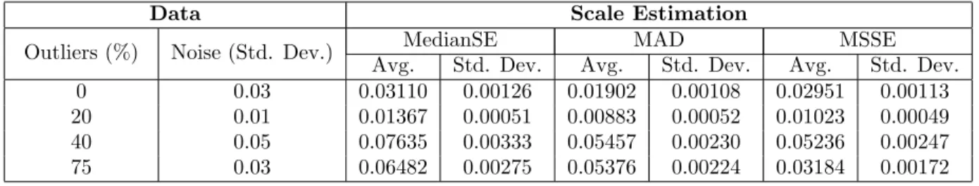
Data Scale Estimation
Outliers (%) Noise (Std. Dev.) MedianSE MAD MSSE Avg. Std. Dev. Avg. Std. Dev. Avg. Std. Dev. 0 0.03 0.03110 0.00126 0.01902 0.00108 0.02951 0.00113 20 0.01 0.01367 0.00051 0.00883 0.00052 0.01023 0.00049 40 0.05 0.07635 0.00333 0.05457 0.00230 0.05236 0.00247 75 0.03 0.06482 0.00275 0.05376 0.00224 0.03184 0.00172 Table 1: Noise scale computation example for points sampled on a plane, corrupted with noise and outliers. The number of input points is 1000, but a percentage of them (1st column) are generated following a unifom random distribution inside a slightly enlarged bounding box, and the inlier points are corrupted with gaussian noise with varying amounts of standard deviation (2nd column). Using the LKS selection for the best model (q = 0.2), the scale is computed using MedianSE, MAD and MSSE. Due to the random nature of LKS, the procedure has been computed 100 times and the mean (Avg.) and standard deviation (Std. Dev.) of the results are shown. Note how MSSE provides a close approximation of the original noise even in the case where the number of outliers is larger than 50%.
N = 293 iterations to have 99% probability of selecting at least one outlier-free set to instantiate the model. The scale measure is then computed from the model.
Given a model computed by the LKS, its residuals can be computed and a scale measure can be extracted from them. There are many possible algorithms for solving the automatic scale estimation problem, two of the most well known are the Median and the Median Absolute Deviation (MAD) (Rousseeuw and Leroy, 1987). While simple to compute, these two methods again have a known breakdown point of 50%. This can be seen in the simple tests reproduced in Table 1. Since we want to be weaker when imposing the minimum number of points forming an LBQ inside our neighborhood, we keep following the idea proposed by MSSE, which consists of iteratively refining the scale measure. Starting from the j-th sorted residual corresponding to j = qk, the noise scale estimate is computed as follows:
σj= Pj i=1r 2 i j − M , (5)
where M is the dimension of the model to fit (i.e., M = 6 for the case of the LBQ).
MSSE is based on the idea that incrementally taking into account more residuals (increasing j) generates σj measures that increase progressively, and a big jump will happen when the added residual comes from a
point of a different model or an outlier, i.e.: r2
j > T 2
σ2
j, (6)
where T is a constant factor, which can be set to T = 2.5 if we assume Gaussian noise (98% of inliers will be identified as such). From equations (5) and (6), the following inequation can be formulated:
σ2 j+1 σ2 j > T 2 − 1 j − M + 1. (7)
Thus, the first outlier can be identified by checking the validity of this inequality, and the scale measure will be the σj−1; that is, the scale estimation previous to finding the big jump.
While it could be possible to compute the noise scale locally inside each C(s), the computational effort it requires would make the method unfeasible. Consequently, previous to the meshing procedure, a scale value is computed for each point in order to alleviate the computational cost. We use a fixed k neighborhood around each point, and compute a scale measure using the procedure defined above. Then, during the meshing, from all the scale values corresponding to the points inside the current C(s), a representative value is computed. In order to do this, we again apply MSSE, but to the set of scale measures associated to the points in C(s). Consequently, this second MSSE step is not computed on residuals. Instead, we seek the first big jump in scales, which also corresponds to finding scales generated from another structure or from any outliers.
5.4
Local Bivariate Quadric - Segment Intersection
With the procedure presented so far, we are able to provide a local surface for each query segment. Thus, the last step needs to find the intersection with this LBQ surface. In order to compute the intersection between s and the LBQ, we cast the segment in its ray form and use its parametric equation:
s(t) = so+ sdt, (8)
where so = (xo, yo, zo) is the starting point of the segment and sd = (xd, yd, zd) its direction. Substituting
equation (8) in (1) results in a general quadratic equation: αt2+ βt + γ = 0. Obviously, we can deduce its
parameters: α = Ax2 d+ By 2 d+ Exdyd β = 2Axoxd+ 2Byoyd+ Cxd+ Dyd+ Exoyd+ Exdyo− zd γ = ax2 o+ By2o+ Cxo+ Dyo+ Exoyo+ F − zo, (9)
and then obtain the two possible solutions for t using the general method. In order to ensure that the solution falls within the segment, we have to verify that t < length(s).
The equations presented so far solve the general segment-LBQ intersection problem. Note however that we have fixed the normal of the fitting plane of the LBQ to coincide with the direction of the segment. Thus, the segment coincides with the fitting axis, and thus just a single intersection may occur. Having xo= yo= xd= yd= 0, the problem formulated in equation (9) simplifies to:
t = − 1 F − zo
(10)
The presented framework provides the intersections against correctly computed LBQs. However, during the computation of the LBQs, some problems may arise. The most obvious is that the structure in C(s) might not be represented using an LBQ. This is the case for the example in Figure 4 (a), where the structure inside C(s) could be too complex to be captured by an LBQ. Another problem emerges from the fact that RANSAC always returns an LBQ regardless of the number of points involved. As mentioned above, one of the parameters used to test the correctness of this surface is to impose a minimum number of points δi agreeing
with it. However, there might be a case like the one depicted in Figure 4 (b), where C(s) comprises some points, but clearly the surface they define is not supposed to intersect the segment since it is a hole. In order to deal with these cases, we only consider as valid the intersection points that are supported. This means that some inlier points must lay close to the intersection point in order to validate it. Thus, a user-defined minimum number of inlier points γiis required to fall inside a sphere centered on the intersection point and
with a radius γfc where 0 < γf ≤ 1, i.e., a fraction of c. Obviously, tunning γi and γf depends on the
sparseness of the data compared to the desired c parameter. This simple heuristic also allows the method to return a null intersection in cases where the local surface represented by the points in C(s) does not intersect the segment, but is close enough so that an LBQ intersecting the segment can be generated in C(s). This is the problem shown in Figure 4 (c), and note that in this specific case, the most supported surface does not intersect the segment but there is another cluster of points defining another local surface that intersects the segment. As presented above, we have to take into account that more than a single structure or LBQ may be contained inside the C(s). For this reason, the model creation/intersection computation process is not unique: if the segment does not intersect the model, another model is computed from the set of remaining points (the outliers of the current model), and an intersection test is carried out again (as shown in Figure 4 (d)). The process stops when a valid intersection is detected, when no more models can be generated, or when a given number of trials is reached (3 in our implementation).
6
Post-Processing
Although the proposed method provides satisfactory results in most cases, variability during intersection computation caused by noise may result in inconsistencies in the reconstructed mesh. It is obvious that we are not imposing any continuity on the surface by just performing local intersection computations. In this sense, the local surface computed in a given part of the model is not continuous with a local surface computed nearby, even if most of the points taken into account are the same. Thus, the RDT mesher may not provide a manifold surface. For this reason, the non-manifold configurations that may arise in the mesh need to be
(a) (b)
(c) (d)
Figure 4: Problematic segment-LBQ intersection configurations: LBQ in grey, inliers as bright/green points and outliers as dark/red points. In (a), the part of the surface contained in C(s) cannot be represented by an LBQ. In (b), the LBQ returned by RANSAC is filling a hole in the data, which is not desirable in most cases. Finally, in (c), the most supported LBQ is constructed from points falling far from the segment, and the computed LBQ is not correct. Note however that, on a second iteration shown in (d), another LBQ will be generated from the set of outlier points, which in this case will clearly intersect the segment.
(a) Non-manifold edge (1) (b) Non-manifold edge (2) (c) Non-manifold vertex
Figure 5: Non-manifold structures, highlighted in each of the meshes presented.
• Non-manifold edges: Edges where more than two triangles meet generated by wrong intersection points detected near the surface. In most cases this aberration can be eliminated by removing the facets incident to the non-manifold edge whose three edges are not shared by another triangle (see Figure 5 (a)). However, this test becomes invalid in the situation where the RDT includes a connected set of 4 facets, forming the boundary of a flat tetrahedron that shares four non-manifold edges with the reminder of the surface (as in Figure 5(b)). The special case is filtered out by selecting, out of these 4 facets, one of the two pair of facets incident along manifold edges.
• Non-manifold vertices: Vertices not surrounded by topological fans. In this case, since is difficult to tell locally which triangles are more likely to be eliminated, all the triangles incident to this vertex are removed.
Examples of these aberrations are illustrated in Figure 5. After filtering all the non-manifold configura-tions, some small sets of triangles may remain unconnected to the global surface. For this reason we remove the small connected components that are not likely to be part of the final surface.
Obviously, the presented manifoldness cleaning step will result in small holes in the surface that need to be filled. Furthermore, due to the large and variate possible cases of intersection between local surface and segment that can occur inside a given C(s), some of the intersection queries may get a wrong result, as detailed in Section 5.4. This also produces some holes in the surface that need to be filled for aesthetic purposes. In order to do so, we use the method presented in Liepa (2003). This method provides the resulting filling to fairly interpolate the missing shape, using triangles with sizes similar to those on the border of the
hole. The method applies 3 sequential steps to each hole. First, a minimum weight triangulation is devised in order to fill the hole linearly. Then, this initial hole-filling triangulation is refined following the apparent density and sizing of the border triangles of the hole. Finally, the triangulation is faired in a way so that the triangulation filling the hole smoothly approximates the shape based on the other parts of the surface surrounding the hole. The small holes to fill in our meshes are automatically detected as the set of border edges forming a closed loop, where this number of edges is smaller than a threshold. This threshold avoids filling large holes corresponding to undersampled parts or the borders of the recovered shape. Note that a procedure similar to the one proposed here (non-manifold configurations removal and hole filling) has shown to provide satisfactory results in Ohtake et al. (2005).
In case of extreme noise, the surface retrieved by our method also presents some roughness in places where the capsule neighborhood associated to the required query segments is not able to fully contain the noise in this part of the data. This is likely to happen when we require the mesher to provide high resolution surfaces, as the query segments may become smaller than the noise scale in an area, such that they may not include inside its capsule neighborhood enough points to create a fully correct LBQ. In order to alleviate these artifacts, we apply a Laplacian smoothing technique (Hansen et al., 2005). This method basically consists of moving each vertex on the mesh to the mean position defined by its neighbors. This smoothing procedure was not used on all the presented results, but only on a few of them (see Table 2) and, when applied, only a single iteration of Laplacian smoothing was enough to reduce the noise.
7
Experimental Results
We prove the validity of the presented pipeline on challenging real underwater datasets from different ap-plication areas. To better illustrate the excellent performance of the method, we briefly overview its be-haviour when applied to both synthetically generated point sets and standard range scan datasets. Then, we rigourously test the method on real underwater datasets, focusing on the problems that optically generated 3D point clouds present in underwater environments and how they affect our method. In Table 2, one can find the parameters used in each execution, while in Table 3 the running times for each of the tested datasets are shown.
7.1
Synthetic
Two small synthetic datasets are reported in this section to show the capabilities of the method under variable noise and outliers. The first dataset consists of a uniform sampling of a unit sphere. The results of our method under ideal conditions are seen in Figure 6 (a). In order to test the method with more realistic conditions, we decided to corrupt the original point set by adding different levels of both Gaussian noise and outliers. Both the data points and the results of our method can be seen in Figure 6 (b-j). Note in Table 2 that we use a more restrictive set of parameters to deal with these corrupted datasets. Moreover, we did not apply any of the post-processing operations presented in Section 6 to obtain the results shown. The reader may observe that for all the noise levels tested, the inclusion of small sets of outliers (i.e., 25%) does not greatly corrupt the reconstructed surface. However, as the outliers corruption increases we obtain rougher surfaces, possibly containing small holes, and with larger number of non-manifold configurations.
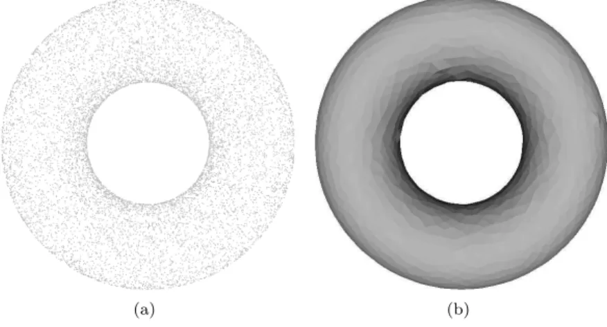
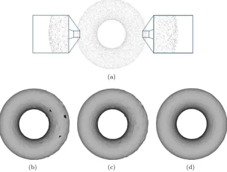
The second synthetic dataset has been generated by sampling a torus, but this time non-uniformly sampled. The point set and its surface retrieved by our method are shown in Figure 7 (a,b). In order to test the behaviour of our method, not only under non-uniform sampling but also under non-uninform noise, we added noise to this dataset that varies from left to right in Figure 8 (a), from σ = 0BBD to σ = 0.005BBD, where BBD stands for the Bounding Box Diagonal of the input points. The behaviour of our method can be seen in Figure 8 (b), where one can notice that the surface is hole ridden and quite bumpy. In this situation, the hole filling procedure, followed by the Laplacian smoothing, allows the method to recover a more pleasant representation of the torus. The results of these two steps can be seen in Figure 8 (c) and (d) respectively.
7.2
Range Scans
Range scanning technology has become a tool of great importance in land robotics systems. High-resolution indoor object reconstruction has also benefitted from the new achievements in range finders. We illustrate the behaviour of our system when applied to some of the benchmark datasets from this kind of sensor. We start with the Max Planck model, a close-to-ideal dataset which is regularly sampled and not corrupted by
(a)σ= 0 / O = 0
(b)σ= 0.01 / O = 25 (c)σ= 0.01 / O = 50 (d)σ= 0.01 / O = 100
(e)σ= 0.025 / O = 25 (f)σ= 0.025 / O = 50 (g) σ= 0.025 / O = 100
(h)σ= 0.05 / O = 25 (i)σ= 0.05 / O = 50 (j)σ= 0.05 / O = 100
Figure 6: The Sphere dataset (10,242 points) shown in (a) is corrupted in subsequent figures by adding different levels of Gaussian noise and outliers. The surface reconstructed by our method, without post-processing, is shown alongside each point set. The σ value represents the standard deviation value for the added noise, while the O value denotes the percentage of randomly uniform distributed outliers added to the original set, inside an slightly enlarged bounding box.
(a) (b)
Figure 7: Using the noise free version (a) of the Torus dataset (10,000 points), the surface on (b) is generated using our method.
(a)
(b) (c) (d)
Figure 8: The noise corrupted version of the Torus dataset (a), causes the surface recovered by our method (b) to be bumpy and defected with holes. The hole filling (c) and smoothing (d) procedures allow the recovery of a more faithful approximation of the original object.
noise. We can see in Figure 9 how in this case the reconstructed surface faithfully represents the object. It is worth noticing that when no noise is present in the data the smoothing step is not required.
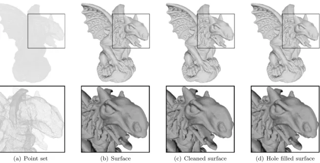
On the other hand, in Figure 10, the effect of the cleaning and hole filling post-processing methods is shown on the Gargoyle dataset. In Figure 10 (b), the raw surface as extracted by our method is presented, where some holes (black spots) are visible. After the non-manifold configurations cleaning step, Figure 10 (c), even more holes appear. After the hole filling, the final surface is presented in Figure 10 (d). On the other hand, we show in Figure 11 the results of other state-of-the-art methods applied to this dataset. The selected methods were Multilevel Partition of Unity (MPU) (Ohtake et al., 2003), Robust Cocone (Dey and Goswami, 2006), Algebraic Point Set Surfaces (APSS) (Guennebaud and Gross, 2007) (its MeshLab implementation (Visual Computing Lab ISTI - CNR, 2005)), and Poisson (Kazhdan et al., 2006). You may observe that all the methods obtain good results for this reference shape.
As previously shown, since the quality of the resulting mesh is user-defined, our method is able to create multiple resolution versions of the same object. In Figure 12, an example of this property applied to the
(a) (b)
(a) Point set (b) Surface (c) Cleaned surface (d) Hole filled surface
Figure 10: The application of our method to the Gargoyle point set (863,210 points) shown in (a) raises the surface in (b), where holes are directly visible as black spots. After the non-manifoldness cleaning step in (c), even more holes appear. By using the hole filling procedure, these small imperfections are corrected, as can be observed in (d).
(a) MPU (b) Robust Cocone (c) APSS (d) Poisson
Figure 11: Results of some of the state-of-the-art surface reconstruction methods applied to the Gargoyle dataset. From left to right, the methods tested are MPU (Ohtake et al., 2003), Robust Cocone (Dey and Goswami, 2006), APSS (Guennebaud and Gross, 2007) and Poisson (Kazhdan et al., 2006). With the exception of Robust Cocone, the methods tested require per-point normals, in this case available from the original range scan data. Note that this reference shape poses no problem to any of the methods, and that the results obtained are comparable to those provided by our method, shown in Figure 10 (d).
(a) (b) (c) (d)
Figure 12: The Elephant dataset (1,537,283 points), shown in (a), is used as input for our method to create multiple surfaces, shown from (b) to (d), at increasing resolution.
(a) (b) (c)
Figure 13: In (a), the Stanford Bunny dataset (362,272 points) is presented. Note in (b) how the recovered surface is quite bumpy near noisier areas. In (c), one can see the usefulness of the smoothing step in these cases.
Elephant dataset is shown.
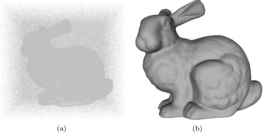
Finally, we apply our method to a noisy dataset, namely the Stanford Bunny, where measurement vari-ability and registration errors are present. In this case, and due to the lack of continuity enforcement on the surface retrieved by our method, the result obtained shows a bumpy surface in the areas where the mentioned errors are more emphasized (Figure 13 (b)). Here, as seen in the Torus point set, the optional smoothing step can be applied to correct the results.
In order to demonstrate the resilience to outliers of our method, and given that these range scans do not usually contain many of these outliers, we corrupted the Stanford Bunny dataset by adding 100% of outliers. These outliers have been added by generating a set of random points uniformly distributed inside the bounding box of the original dataset slightly enlarged by 5%. The results can be seen in Figure 14, where one can see that the method is still able to provide a correct reconstruction. Note how even in the presence of this vast amount of outliers, the results provided by our method are similar to those ones presented in Figure 13 (c).
In underwater robotics, range sensors come in the form of multibeam sonar. In order to demonstrate the versatility of the presented method, we show the behaviour of the method when applied to multibeam sonar scans. Contrary to most multibeam surveys, it is not that obvious in this case whether there is a plane proxy where this raw point set could be approximated using a 2.5D heightmap (check its structure in Figure 15, left). Thus, a method working on unconstrained 3D like the one presented might be more desirable in order to reconstruct a surface mesh from these points. The applicability of our method is demonstrated
(a) (b)
Figure 14: (a) shows the Stanford Bunny dataset, corrupted with 100% of uniform randomly distributed outliers (724,544 points), while (b) presents the resulting surface as retrieved by our method.
Figure 15: Multibeam sonar reconstruction (413,873 points). Instead of the standard downward-looking configuration, the transponder was installed laterally, giving rise to a full 3D dataset.
in the right part of Figure 15, where the recovered surface is presented. This application sets the path for the development of sonar scanning of underwater structures in more general configurations than the typical downward/forward viewing with respect to the scene.
7.3
Underwater Multi-view Stereo Datasets
Finally, in this section we present the results of our method when applied to optical multi-view seafloor reconstruction. The optical reconstruction technique used to retrieve the point set used as input for our method is a common multi-view plane sweeping technique similar to the one in Yang and Pollefeys (2003). This kind of technique provides a dense representation of the scene, as each image contributes to the point set with a dense depth map. However, the outliers of each depth map accumulate for each view. Furthermore, reconstructing each depth map separately for each view does not enforce coherence between them, which translates into double contours when registration errors are present. Finally, in order to take advantage of the richness provided by the texture in the images, we also present for each dataset its texture-mapped version. For each triangle in the model, we use the texture corresponding to the view that maximizes the projected area in image space. This simple technique has proven to be useful in the underwater media (Garcia et al., 2011), as it offers a good tradeoff between the orthogonality of the view direction with respect to the orientation of each triangle and promotes views taken closer to the scene, i.e., less affected by the absorption and scattering of the medium.
Figure 16: Shallow water dataset reconstruction. From first to last row: point set (1,856,271 points), meshed surface, and textured surface.
in shallow waters. This shallow-water dataset presents an almost ideal scenario, as the common challenges appearing in underwater imaging are not present. As can be seen in Figure 16, our method is able to extract a smooth surface under these conditions, preserving the fine details of the scene.
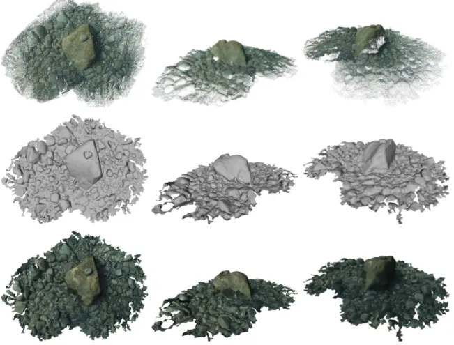
A more complicated dataset, also covering a larger area, is presented in Figure 17. This dataset consists of a survey of a coral reef, acquired at a relatively low depth. Even if the illumination conditions are not a problem, the retrieved point set presents a clear example of non-uniform sampling. This poses a challenge to our algorithm, since undersampled areas result in more holes in the surface. In this case, we decided not to fill them in the final meshed surface, as some holes are connected to the surface boundary and would require filling the entire boundary where the sampling of the surface ends. Taking a closer look at the places where the sampling is unsatisfactory, one can see that they correspond to vertical walls. These vertical walls were only shallowly observed during the survey, since a downward-looking camera configuration was used. This resulted in fewer samples covering those areas, promoting the dramatic change in the sampling rate between the top of these mound-like shapes and their lateral parts.
In the optical datasets shown so far, the survey of the scene has been carried out with a downward-looking configuration. This does not demand the application of our method, as an approximation in the form of a height map could also be provided, preserving more or less the overall shape of the scene. However, the case illustrated in Figure 20 presents a more general camera configuration for the survey of an underwater hydrothermal vent. This hydrothermal vent, called the Tour Eiffel, has been the target of many geological, chemical and biological studies in the last decade (Langmuir et al., 1997). It is located on the Mid-Atlantic Ridge, at around 1700m depth, and is more than 15m high. Obviously, the details of this intrincate shape cannot be recovered using the common downward-looking configuration. In this case, the survey was carried out using a forward-looking camera configuration, with the robot going around the object several times (see the camera trajectory in Figure 1). Note in Figure 18, how the input sequence is more challenging than
Figure 17: Coral reef dataset reconstruction. From first to last row: point set (1,656,413 points), meshed surface, and textured surface.
in the other cases, as the attenuation of the light with distance is strong, and the high depths at which it was collected forced the use of artificial lightning, causing non-uniform illumination across the images and emphasizing the blurring and scattering produced by suspended particles in the medium. Due to these phenomena, the point set retrieved is noisier and presents several outliers, as depicted in more detail in Figure 19. However, in Figure 20 we can see that even in this case our method obtains a correct surface following the main shape, at the same time disregarding the outliers. In order to validate the output of our method, we compared our results with those of some of the methods in the state of the art. The first row in Figure 21 shows the resulting meshed surfaces after applying the most relevant methods, which correspond to those also tested on the Gargoyle dataset in Figure 11. Given the global view of these methods, they are able to deal with outliers to some extent. However, the vast number of outlier points posed by this dataset doomed them to failure. The result obtained by MPU, illustrated in Figure 21 (a), shows a spiky surface that does not resemble the object visible in the original image sequence, and also some hallucinated off-surfaces created due to outliers. In Figure 21 (b), we can observe that the surface retrieved by the Robust Cocone method encloses most of the points (including the outliers), giving rise to a hull whose triangles do not pass near the denser parts of the original point set, where the surface is actually described. All the same, the results of the APSS method in Figure 21 (c) are similar to the MPU case, presenting again a bumpy mesh that does not resemble the expected surface. Finally, in Figure 21 (d), one can find the results for the Poisson method (Kazhdan et al., 2006), a widely used and cited method nowadays. Compared to the other methods, it achieves a better reconstruction in the sense that most of the object’s shape is correctly recovered as a smooth surface. However, it also shows a nonexistent off-surface at the back of the model that should be filtered manually. It is worth noting that, except for the Robust Cocone method, all the presented methods require oriented point sets, i.e., a normal for each point must be known. For all the cases presented, normals have been computed using the method of Hoppe et al. (1992) using a k = 100, which we found to be a good tradeoff given the number of points in the dataset and its noise. However, note that since outlier points may also have erroneous normals associated in some areas of the object, this makes the method behave erratically on these parts. On the contrary, our method works directly with the raw point sets.
We present next an even noisier dataset corresponding to a survey of a shipwreck of the XVIIth century
Figure 18: Three sample images of the Tour Eiffel sequence (from a total of 928). This challenging sequence presents common problems in underwater imaging: blurring, attenuation of light with distance and scattering.
Figure 19: Close-up on the point set of the Tour Eiffel dataset (1,368,115 points). Note the high number of outliers.
Figure 20: The Tour Eiffel dataset, reconstruction of an underwater hydrothermal vent. From first to last row: point set, meshed surface, and textured surface. Note how the surface is correctly reconstructed even in presence of a high number of outliers.