HAL Id: halshs-00594051
https://halshs.archives-ouvertes.fr/halshs-00594051
Submitted on 18 May 2011
HAL is a multi-disciplinary open access archive for the deposit and dissemination of sci-entific research documents, whether they are pub-lished or not. The documents may come from teaching and research institutions in France or abroad, or from public or private research centers.
L’archive ouverte pluridisciplinaire HAL, est destinée au dépôt et à la diffusion de documents scientifiques de niveau recherche, publiés ou non, émanant des établissements d’enseignement et de recherche français ou étrangers, des laboratoires publics ou privés.
Sophie Bernard
To cite this version:
Centre d’Economie de la Sorbonne
Remanufacturing
Sophie BERNARD
Sophie Bernard
yUniversity Paris 1 Panthon-Sorbonne, Paris School of Economics, Centre d’économie de la Sorbonne
April 13, 2011
Thanks to the editor and the two anonymous reviewers for their invaluable comments. Special thanks to Louis Hotte, Stan Winer, Gamal Atallah, Hassan Benchekroun, Mireille Chiroleu-Assouline, Mouez Fodha, Denis Claude and seminar participants at University of Ottawa, 5th CIREQ Ph.D. Students’ Conference, University of Paris 1 Panthéon-Sorbonne, the 19th Canadian Resource and Environmental Economics Study Group (CREE) and the 4th World Congress of Environmental and Resource Economists (WCERE). Research supported by the FQRSC (Fonds québécois de recherche sur la société et la culture).
yEmail: [email protected]. Address: Maison des Sciences Economiques, 106-112
This paper presents a theoretical model of remanufacturing where a duopoly of original manufacturers produces a component of a …nal good. The speci…c component that needs to be replaced during the lifetime of the …nal good creates a secondary market where independent remanufacturers enter the competition. An environmental regulation imposing a minimum level of remanufacturability is also introduced. The main results establish that, while collusion of the …rms on the level of remanufactura-bility increases both pro…t and consumer surplus, a social planner could use collusion as a substitute for an environmental regulation. However, if an environmental regula-tion is to be implemented, collusion should be repressed since competiregula-tion supports the public intervention better. Under certain circumstances, the environmental regulation can increase both pro…t and consumer surplus. Part of this result supports the Porter Hypothesis, which stipulates that industries respecting environmental regulations can see their pro…ts increase.
Keywords: remanufacturing, competition, environmental regulation, Porter Hy-pothesis.
Ce papier présente un model théorique de remanufacturing où un duopole de man-ufacturiers originaux produit un composant d’un bien …nal. Ce composant devant être changé, un marché secondaire est créé. Une réglementation environnementale déterminant un niveau minimal de remanufacturabilité est introduite au modèle. Les principaux résultats indiquent d’une part que la collusion des …rmes sur le niveau de remanufacturability augmente les pro…ts et le surplus du consommateur et d’autre part qu’un plani…cateur social pourrait substituer la réglementation environnementale par la collusion. Cependant, lorsqu’une réglementation environnementale est prévue, la collusion devrait être réprimée puisque la compétition s’accorde mieux avec une inter-vention publique. Sous certaines conditions, la réglementation peut aussi augmenter les pro…ts et le surplus du consommateur. Une partie de ces résultats coïncide avec l’hypothèse de Porter stipulant que les industries soumises à des réglementations envi-ronnementales peuvent voir une augmentation de leurs pro…ts.
Mots clés: remanufacturing, compétition, réglementation environnementale, hy-pothèse de Porter.
1
Introduction
Remanufacturing is a speci…c type of recycling in which used durable goods are repaired to a like-new condition. Both remanufacturing and recycling avoid post-consumption waste while reducing the use of raw materials. However, recycling is an energy-intensive process that conserves only material value. In attempting to meet multiple environmental objectives, remanufacturing can be a more suitable option; it preserves most of the added-value by giving a second life to the product and, typically, reduces the use of energy by eliminating production steps. This paper develops a model of remanufacturing where a government may either favor an environmental collusion between producers or introduce an environmental regulation setting a minimum level of remanufacturability. The impact on pro…ts and consumer surplus is analyzed.
The level of remanufacturability de…nes the technical attributes that facilitate the product reuse and refurbishing at the end of its life. In this sector, waste reuse becomes a design objective, so that remanufacturability can be seen as a form of green design. Moreover, since it deals with end-of-life product management and recycled materials, remanufacturing
belongs to the eco-industry as de…ned by the OECD and Eurostat.1
After a product’s …rst life, recycled material can be redirected towards any industry. On the contrary, the material going through the remanufacturing process goes back to the same industry. Then, remanufacturing-oriented designs permit the original manufacturers (OMs) to access the secondary market’s bene…ts. Indeed, while remanufactured products are sold at 60 to 70 percent of the new products’price, their production accounts for only 35 to 60 percent of the original costs [Giuntini and Gaudette 2003]. Therefore, when new products can
1Eco-industries "[...] include cleaner technologies, products and services which reduce environmental risk
and minimize pollution and resource use." [“The Environmental Goods and Services Industry: Manual for Data Collection and Analysis” OECD, 1999]
For an introduction to the literature on green design see Fullerton and Wu (1998), Eichner and Pethig (2001) and Eichner and Runkel (2005). For the literature on eco-industry, see David and Sinclair-Desgagné (2005) and Canton (2008).
be substituted with remanufactured ones, original manufacturers may undertake pro…table remanufacturing initiatives. Xerox, Kodak, Ford Motor Company and Mercedes-Benz are examples of corporations that could reduce their production costs with voluntary product recovery [To¤el 2004]. These corporations are part today of a 60-100 billion dollar industry according to the sources.
In this framework, the car parts industry is of particular interest. Combined, alternators and starters represent 80 percent of remanufactured products [Kim et al. 2008]. Valeo and Bosch are two important alternator producers in Europe. They started remanufacturing activities in the early 90’s, following the announcement of legislation prohibiting the
produc-tion, sale and use of asbestos2: a technological constraint that has made alternator
reman-ufacturing commercially viable. Remanufactured alternators and starters are produced at a fraction of the original cost. Steinhilper (1998) shows that on average they require 14% of the energy and 12% of the material necessary for the production of new ones. Representative of the remanufacturing industry, this reduction in energy and raw material consumption makes remanufacturing both environmentally desirable and industrially pro…table. Inspired by the alternator anecdote, one of the main purposes of this paper is to describe how green designs can be costly for the industry and become pro…table once an environmental regulation is introduced.
Over the years, pro…tability concerns have made remanufacturing a hot topic in the en-gineering and managerial worlds, witness the ‡ourishing literature on reverse logistic, stock
planning, material demand and return, and case studies.3 Nonetheless, there are only a
hand-ful of economic studies that consider the e¤ect of public interventions on remanufacturing activities [Webster and Mitra 2007; Mitra and Webster 2008].
The current paper proposes a theoretical model of remanufacturing framed on the
partic-2This legislation was enacted in 1993 in Germany and in 1997 in France, the respective headquarters of
Bosch and Valeo, with the European Union following suit in 1999 [European Commission 1999].
3See for instance Ferrer (1997), Kiesmuller and Laan (2001), Majumder and Groenevelt (2001), Lebreton
ularities of the alternator industry. A duopoly of OMs compete on the primary market where they face the threat of an outsider; they also compete on the aftermarket where consumers of remanufactured products may alternatively use the services of competitive independent remanufacturers (IRs). The model pins down the di¤erent incentives in the technology selec-tion determining the level of remanufacturability and explores the consequences of environ-mental regulations. Particularly, it explains why original alternator manufacturers refrained from adopting a voluntary withdrawal of asbestos from their production in order to launch pro…table remanufacturing activities.
Most previous research works have assumed a …xed level of remanufacturability. A study by Debo et al. (2005) analyzes the technology selection for remanufacturable goods when
a higher level of remanufacturability may invite entry by IRs.4 Stronger competition on
the remanufacturing market pulls down prices and OMs show lower interest in costly pro-duction technology. Therefore, governmental interventions promoting competition on the aftermarket have an adverse e¤ect on the level of remanufacturability. This corroborates the observation of Ferrer (2000) who states that remanufacturing is viable only if the re-manufactured product is priced above its marginal cost. Following Debo et al. (2005), the current model considers the positive one-way externality of remanufacturability on IRs. However, OMs can endogeneously choose among a range of existing technologies and reduce, for low levels of remanufacturability, the impact of technological spillovers. Also, studies that observe e¤ects of competition on the remanufacturing market generally assume away
competition on the primary market; i.e. they assume a monopolistic original manufacturer.5
The current model innovates by considering a duopoly and the threat of an outsider. One
4Since remanufacturability gives the products a positive value at the end of their life, OMs have the
incentive to o¤er remanufacturable products when the end of life value is re‡ected in the original product price.
5See for instance Carlton and Waldman (2009), Mitra and Webster (2008), Debo et al. (2005) and
Majumder and Groenevelt (2001). In a di¤erent context, Heese et al. (2005) study a duopoly that compete on the primary market. In their model, new products have a positive initial remanufacturability level. Hence the …rst mover in launching take-back strategy can deter the competitor by o¤ering a new product with a lower price that includes a discount for the consumer who will return the used product.
major point that distinguishes the current model from the previous literature is the per-fect market segmentation between new and remanufactured products. In an industry where there is a need for compatibility between the component and the …nal good, and where the component can be remanufactured several times, the need for new good production on the aftermarket is negligible. In the alternator industry, more than 90% of the aftermarket is …lled with remanufactured products.
Other literatures that can be used to understand this remanufacturing market include the literature on durable goods with repeated purchases as well as the economics of innovation in the presence of technological spillovers. These topics will be discussed below.
Finally, similarities between recycling and remanufacturing are such that they use com-parable public interventions. Webster and Mitra (2007) and Mitra and Webster (2008) have pointed out that take-back regulations as well as subsidies can encourage remanufacturing activities. These tools have also been studied in the recycling literature [Fullerton and Wu 1998; Eichner and Pethig 2001; Eichner and Runkel 2005; To¤el et al. 2008]. Furthermore, because recyclable and remanufacturable products present common characteristics in their conception [Steinhilper 1998], regulations aimed at either recycling or remanufacturing may interchangeably foster one activity or the other.
The main results show that in the absence of environmental regulation, collusion leads to a higher level of remanufacturability while increasing both pro…ts and consumer surplus. When remanufacturability is environmentally desirable, the government may use collusion on the level of remanufacturability as a substitute for an environmental regulation. In the absence of public intervention, the threat of entry on the primary market sticks the original price at the production cost of non-remanufacturable products. Consequently, the OM who decides to produce remanufacturable goods must absorb the full cost of remanufacturing-oriented technologies. This phenomenon explains what has refrained alternator producers to adopt remanufacturable technologies prior to the regulation on asbestos. The introduction of an environmental regulation imposing a minimum level of remanufacturability reduces
the threat of the outsider, since potential entrants will be subjected to the same regulation. Softened market competition leads to an increase in the original product price and corre-spondingly higher OMs pro…ts. This result is in line with the Porter Hypothesis stating that environmental regulations may increase pro…ts in regulated industries. Finally, under speci…c circumstances, an environmental regulation can also increase consumer surplus.
The model is introduced in the next section, which sets technologies, demands and the industrial structure. Section 3 completes the assumption on technology and describes the optimization problem for two cases: non-cooperation and collusion. Section 4 observes the e¤ect of an environmental regulation. Section 5 concludes.
2
The Model
A duopoly of identical original manufacturers (OMs) produce an intermediate good m (the alternator), which enters as a component of a …nal consumption good (the vehicle). This constitutes the primary market and the component’s …rst life. Since the same car goes through two or three alternators [Kim et al. 2008], the lifetimes of the alternator and the vehicle are respectively l and L, with l < L. Consequently, consumers of the …nal good all have to replace the defective component at each of the b replacement periods, where
b = (L=l) 1. This creates an aftermarket.
The alternator’s original life aims speci…cally at the new vehicle industry with one al-ternator per vehicle. Used alal-ternators can be remanufactured several times and, at any moment, there are an equal number of cars and alternators on the market.
When they originally produce a remanufacturable component, OMs participate in the aftermarket by recovering and remanufacturing used products. On this market, however, they face competition from independent remanufacturers (IRs). In 2005, IRs represented
54% of the aftermarket for automotive parts in Europe and 66% worldwide.6
2.1
Technology
Each OM i, i 2 f1; 2g, controls its level of remanufacturability qi, a technology choice
corresponding to the ease with which a used product can be remanufactured7 and leading
to decreasing unit remanufacturing costs cr(qi) and cs(qi), for OMs and IRs respectively.
However, OMs bene…t from economies of scope between new and remanufactured products8
and, for any given q, have lower unit remanufacturing costs than IRs. This technological advantage for OMs over the IRs is represented by the following properties:
cs(q) cr(q) 0; and asymptotically: lim
qi!1
(cs(q) cr(q)) = 0: (1)
For large levels of remanufacturability, remanufacturing becomes equally accessible for IRs. To make the original product more remanufacturable, OMs bear additional production
costs re‡ected by an increasing and convex initial manufacturing cost, cm(qi).
2.2
Demand functions
The demand for the component is segmented into two types: the demands for new and for remanufactured products.
The demand for new products m is driven by …nal good producers. It is assumed that any variation in the original component price represents a small share of the …nal good production cost and, hence, the demand for m stays inelastic for a reasonably large range of
http://www.apra-europe.org.
7In most models [see for instance Debo et al. 2005; Majumder and Groenevelt 2001; Ferrer and
Swami-nathan 2006] the level of remanufacturability is the percentage of remanufacturable used products. While the share of un-remanufacturable cores can exceed 30% for certain products, it is less than 15% for alternators [Kim et al. 2008]. In the present model, this number is assumed to be negligible so that the alternator/vehicle ratio stays equal to 1.
8Carlton and Waldman (2009) also assume economies of scope between the production of new parts and
prices (or until a certain choke price). Except for great demand elasticities, this assumption does not a¤ect the results, but lightens the model. For simplicity, m is normalized to 1.
The demand for remanufactured products comes from …nal consumers. Since the price of alternators remanufactured by OMs is between 50 to 60% of the price of new alternators
[Kim et al. 2008], it is assumed that consumers always opt for remanufactured products.9
Indeed, remanufactured starters and alternators cover more than 90% of the replacement
market [Steinhilper, 1998]. Consumer types are uniformly distributed over 2 [0; 1], where
+ is the willingness to pay for a replacement good. The positive constant indicates
that even individuals from the lower bound are willing to pay a positive amount. When remanufacturing used products, OMs provide the properties and warranty of new goods while
IRs supply products of lower quality.10 As a result, consumers will express lower willingness
to pay for IRs’ products. The parameter 2 [0; 1] re‡ects this perceived depreciation in
quality.
At each replacement period, individuals maximize their consumer surplus by purchasing a product coming from an OM, an IR or no product at all. This maximization problem is
given by: max[ + pr; (1 ) + ps; 0], where pr and ps are respectively the selling
price of OMs and IRs’ products. Because the component price represents a small fraction
of the …nal good’s value, ps mimics the inelastic aftermarket and ensures that everyone
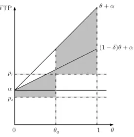
consumes a replacement good; that is, r + s = 1, where variables r and s designate the demand for components remanufactured by the OMs and the IRs respectively. Figure 1 illustrates the willingness to pay for the two di¤erentiated products.
9In other models, two scenarios generally bring new products on the aftermarket. In the …rst one,
products di¤erentiation leads to a positive demand for new replacement products (for instance, in the case of rapid obsolescence like in the computer market). In the second one, the elastic aftermarket demand cannot be ful…lled solely with remanufactured products (like in the disposable camera market). In the alternator industry, the need for compatibility makes product di¤erentiation negligible between new and remanufactured products. Also, the potential supply of remanufactured products correspond to the potential demand since there is one alternator per vehicle and each alternator can be remanufactured several times.
10For the same two year warranty, OMs’ remanufactured products are twice the price of IRs’ products
[Kim et al. 2008]. This suggests a di¤erence in quality. For instance, IRs’products may require more visits to the mechanic.
Figure 1: Willingness to pay and consumer surplus
The set of consumers buying remanufactured products from the OMs is de…ned by such
that + pr (1 ) + ps, or equivalently: (pr ps) = . In Figure 1, given
prices pr and ps, individual q is indi¤erent between the two products. Types 2 [ q; 1]
prefer OMs’services while the others, 2 [0; q], purchase lower quality goods. The shaded
area corresponds to the total consumer surplus at each replacement period.
Given a uniform distribution for , the demand for products remanufactured by the OMs
at each period is r = 1 (pr ps) so that the inverse demand function is:
pr = (1 r) + ps: (2)
For any positive value of the parameter , this depicts the observed price di¤erence between alternators remanufactured by the OMs and the IRs. This premium adds an incentive to the OMs that stays unexplored in the literature.
2.3
Industrial structure
Competition in the industry is described by the following four-stage game. In the …rst stage, two identical OMs produce the original component and control its level of
remanufac-turability qi. Two di¤erent competitive environments will be considered in determining qi:
non-cooperation and collusion. These scenarios internalize, or not, the fact that …rms can
free-ride on each other’s technology selection qi.11
In the second stage, OMs set the original product’s prices and quantities pmiand mi. They
face the threat of an outsider that would seize any pro…t opportunities originating from the
original market but who stays blind on what occurs on the remanufacturing market.12 This
threat forces price competition between OMs, re‡ecting the automotive industry: original components being perfectly substitutable, vehicle manufacturers can switch from one supplier to the other as soon as a lower price is o¤ered.
The third and fourth stages occur on the aftermarket. Although this market is shared with IRs, OMs hold an oligopolistic power on high quality products. In the third stage,
OMs compete by choosing quantities ri. In the …nal stage, IRs compete perfectly and their
remanufactured good’s price is established.
Because of the inelastic aftermarket size, it is assumed that OMs and IRs cannot dis-criminate between products that have di¤erent levels of remanufacturability (everything has to be remanufactured).
OMs have perfect knowledge of each other. Their decisions in each stage are made and applied simultaneously. They also have perfect information about IRs’characteristics. Since
11It has been observed in the alternator industry that i ) Bosch remanufactures Valeo’s alternators; ii )
Valeo remanufactures Bosch’s alternators; and iii ) although, for a given vehicle model, alternators must meet standards set by the automobile constructor, Bosch and Valeo’s products are not identical.
12Two arguments are proposed in order to explain this behaviour. The …rst one assumes that reputation
is an important factor in being considered as an OM and, therefore, new entrants cannot bene…t from a price premium on the aftermarket. The second point considers that incumbents face less risk and are more willing to accept delayed pro…ts.
OMs are identical, a symmetric subgame-perfect equilibrium in pure strategies in the four-stage game is computed.
3
The optimization problem
Under the market clearing conditions, m1+m2 = 1and r1+r2 = r. The OMs’pro…t function
depends on both their activities on the primary market and the remanufacturing market:
i = (pmi cm(qi))mi+ b X t=1 t l[(pr micr(qi) mjcr(qj))ri] | {z } Ri(ri;rj;mi;mj;qi;qj) for i = 1; 2 and j 6= i
where pr= (1 r) + ps from equation (2) and 0 < l < 1 is the discount factor associated
with the length of time l. The …rst term is the net pro…t from the original market while
Ri(ri; rj; mi; mj; qi; qj) corresponds to the discounted pro…t from all the remanufacturing
periods. Because used products randomly go to any remanufacturer, the remanufacturing cost depends on the technology selection of each OM and is weighed by their respective participation in the original market.
3.1
Prices and quantities
Using backward induction, the …nal stage is solved …rst. IRs are perfectly competitive and
the selling price ps is set at the average unit cost of remanufacturing:
ps= mics(qi) + mjcs(qj): (3)
In the third stage, each OM i maximizes its pro…t on the aftermarket by choosing its
supply of remanufactured products ri, and by taking the supply choice of its opponents rj
through equation (3). The OMs maximization problem at this stage is: max ri 0 Ri = b X t=1 t l[( (1 (ri+ rj)) + mi(cs(qi) cr(qi)) + mj(cs(qj) cr(qj)))ri] for i = 1; 2 and j 6= i
and the …rst-order condition is: @Ri @ri = 0 () b X t=1 t l[ rj 2 ri+ mi(cs(qi) cr(qi)) + mj(cs(qj) cr(qj))] = 0: (4)
The Nash equilibrium for the supply of remanufactured products is de…ned by:
ri(mi; mj; qi; qj) =
+ mi(cs(qi) cr(qi)) + mj(cs(qj) cr(qj))
3 for i = 1; 2 and j 6= i (5)
and the second-order condition for an interior maximum is respected when evaluated at the
equilibrium ri.
Here, IRs play a passive role since their price is driven by the OMs’choice of remanufac-turability (equation 3). Also, they only have a residual participation in the aftermarket; the
demand for their products depends on OMs’supply decisions with s = 1 2ri. Note that
the choice of 2ri also corresponds to OMs’aftermarket share.
In the second stage, the two OMs compete on the primary market where the threat of
the outsider keeps the component price pmi at the minimum production cost; that is,
pm1= pm2 = cm(0): (6)
By o¤ering a common original price, OMs share this market equally with mi = 1=2. If a
higher price is set, the outsider, by proposing the lowest level of remanufacturability, can make a strictly positive pro…t and deter competitors. Note that in spite of that restriction, OMs may still optimally choose a positive level of remanufacturability and, consequently,
run a de…cit on the primary market (pmi cm(qi) = cm(0) cm(qi) 0). This is consistent with the existing literature on durable goods with switching costs. In the current model of repeated purchases, the need for compatibility between the component and the …nal good induces a consumer cost of switching to other models of alternators. One standard result
shows how switching costs cause a price war for initial market share.13 Here, …xing the
original price at the lowest production cost prevents the entry by the outsider and secures the original market to the duopoly.
Two situations are considered for the determination of qi and qj in the …rst stage. The
…rst case re‡ects the non-cooperative problem that occurs when an OM remanufactures used products from random origin and free-ride on the technology selection of the other. The second case considers the possibility of an agreement between the OMs. These situations are explicitly formulated in subsections 3.3 and 3.4.
Before solving for the choice of remanufacturability, an important assumption on the technology selection is introduced in the coming subsection.
3.2
Assumption on the technology selection
At this step, only the …rst stage equilibrium remains to be solved and everything thereafter
depends on the technology selection (qi; qj) taken as given. The pro…t function is:
i = (cm(0) cm(qi)) 1 2+ b X t=1 t l[ ri(qi; qj)2] | {z } Ri(qi;qj) (7)
13See Klemperer (1995) for an introduction to the literature. The author relates the example of banks,
giving free banking services to college students. Students who open current accounts are then charged high fees once they graduate. Expected pro…ts in subsequent periods induce a price war for initial market share.
where the optimal supply of remanufactured products (equation 5) is reduced to: ri(qi; qj) = + cs(qi) cr(qi) 6 + + cs(qj) cr(qj) 6 (8)
when the individual market share in equilibrium, mi = 1=2, is taken into account.
A variation in q a¤ects the pro…t through two channels: i) the original production cost
cm(qi); and ii) the total net revenue of remanufacturing activities Ri(qi; qj). Since OMs are
identical, the analysis will focus on symmetric equilibria qi = qj = q. OMs know that, for
any given q, their pro…t depends substantially on their technological advantage: cs(q) cr(q).
The comparative static @ri
@q =
c0s(q) c0r(q)
3 (9)
indicates that, with an increasing technological advantage, a higher level of remanufactura-bility leads to a larger aftermarket share and, consequently, higher remanufacturing revenues.
The following assumption completes the description of the technological advantage intro-duced in section 2.1. It is assumed that OMs have access to a wide range of remanufacturable and substitutable technologies. In dealing with the fact that IRs bene…t from the positive
externality of remanufacturability (through c0
s(q) < 0), OMs endogeneously rank order
tech-nologies with respect to their marginal technological advantage, c0s(q) c0r(q). In other
words, OMs will prioritize technologies where their relative cost reduction is the largest.
Consequently, for low levels of remanufacturability, c0s(q) c0r(q) is positive and large. This
is because the wide technology choice allows OMs to shape the original product in order to
suit their own remanufacturing facilities or assembly lines.14 As the level of
remanufactura-14For instance, in the toner cartridge industry, some …rms have added an electronic key in their
remanu-facturable cartridges that must be reset by the OM. This leads to an increase in the relative remanufacturing cost of IRs [Majumder and Groenevelt 2001].
bility goes higher, the range of technology choices lessens and c0
s(q) c0r(q)decreases. As long
as c0
s(q) c0r(q) > 0, OMs have an incentive to choose higher levels of remanufacturability
since it increases their aftermarket share (see equation 9). At some q = bq, higher levels of
remanufacturability leads to the adoption of technologies that reduce their aftermarket share with c0
s(q) c0r(q) 0. This situation occurs for instance when a larger q eliminates
disassem-bly or reassemdisassem-bly steps originally costlier for IRs.15 For high levels of remanufacturability,
q >q, OMs are constrained with end of tail technologies, i.e. non-substitutable technologiese
speci…cally designed for high performance. Beyond q, higher levels of remanufacturabilitye
slowly reduce the gap between OMs’and IRs’remanufacturing costs. Formally, with bq <eq;
the technological advantage is described by equation (1) and:
c0s(q) c0r(q) 8 > > > < > > > : > 0 for q <bq = 0 for q =bq 0 for q >qb and c00s(q) c00r(q) 8 > > > < > > > : < 0 for q <eq = 0 for q =eq 0 for q >eq (10)
This assumption is in line with a broader literature on innovation. The …rst part, when c0
s(q) c0r(q) > 0, shows the predominance of post-innovation competitive advantage while
the second part, when c0s(q) c0r(q) 0, is the result of an increasing relative rate of
technological spillovers.16 The presence of IRs therefore determines, through technology, the
extent to which OMs reach the aftermarket. Variation of the technological advantage with the level of remanufacturability is illustrated in Figure 2.
15By the mean value theorem, c0
s(q) c0r(q) 0; for at least some q; is an essential condition for the respect
of equation (1).
16See for instance d’Aspremont and Jacquemin (1988) or Celleni and Lambertini (2009). Goel (1990)
studies the R&D decision of a Stackelberg leader (the OMs here) when the follower (the IRs here) bene…ts from one-way spillovers. The author argues that the leader sustains a dominant role when R&D investment implies a greater cost reduction than for the follower. In the current model, that is c0
Figure 2: Technological advantage
3.3
The non-cooperative case
Each manufacturer i maximizes its pro…ts by choosing the level of remanufacturability qi,
taking the technology choice of the other qj as given and considering the optimal supply of
remanufactured products ri(qi; qj). Used products are randomly dispatched among
reman-ufacturers (both OMs and IRs) and, therefore, the technology selection of i is subject to free-riding. The maximization problem is:
max qi 0 i = (cm(0) cm(qi)) 1 2 + b X t=1 t l ri(qi; qj)2 for i = 1; 2 and j 6= i s.t. ri(qi; qj) = + cs(qi) cr(qi) 6 + ( + cs(qj) cr(qj)) 6 ,
and the …rst-order condition is:
@ i @qi = 0 () c 0 m(qi) 2 + b X t=1 t l 2 (c0 s(qi) c0r(qi)) 6 ri(qi; qj) = 0 for i = 1; 2 and j 6= i
where the marginal cost of a higher level of remanufacturability is equal to the marginal revenue generated when the choice of the other is taken as …xed. The symmetric Nash
equilibrium qnc is de…ned by:
c0m(qnc) + b X t=1 t l 2(c0 s(qnc) c0r(qnc)) 3 ri(qnc) | {z } R0(qnc) = 0 (11)
where the subscript nc stands for the non-cooperative case. It is assumed that the second-order condition for an interior maximum is respected when evaluated at the symmetric
equilibrium qnc.17 In the presence of a corner solution q
nc = 0, the component is not
reman-ufacturable.
A positive qnc denotes voluntary remanufacturing activities in the industry.
3.4
The collusive case
In this scenario, OMs agree on a unique level of remanufacturability qi = qj = qc, where the
subscript c refers to the collusive case. OMs internalize each other’s free-riding behaviour by
choosing the level of remanufacturability qc that maximizes joint pro…t (however they still
su¤er from IRs’free-riding activities), which becomes:
max q 0 1+ 2 = (cm(0) cm(qc)) + 2 b X t=1 t l[ ri(qc)2] (12) s.t. ri(qc) = + cs(qc) cr(qc) 3 .
17The second-order condition is c00
m(qnc)+ R00(qnc) 0. For any given q, R00(q) =
Xb t=1 t l h 2 3 (c00 s(q) c00r(q)) 3 ri(q) + (c0 s(q) c0r(q))2 3 i
. From the speci…cations of equation (10), the condition is satis…ed in a large neighbourhood of q =bq. Note that if c00
s(q) c00r(q) is monotonically increasing for q <eq,
The …rst-order conditions is: @ i @q = 0 () c0m(qc) 2 + b X t=1 t l 2(c0s(qc) c0r(qc)) 3 ri(qc) | {z } R0(q c) = 0 (13)
and it is assumed that the second-order condition for an interior maximum is respected when evaluated at qc.18
3.5
Welfare analysis
The consumer surplus is now compared for the two scenarios. Here, consumer surplus on the original market is ignored since prices and quantities stay unchanged. Referring to Figure
1, the consumer surplus on the aftermarket is de…ned by: Sr =
Xb t=1 t l hR1 q( + pr)@ +R q 0 ((1 ) + ps)@ i
: Markets clear in equilibrium, therefore 1 q = 2ri. Using
(2), (3) and (8), the total consumer surplus for a given q becomes:
Sr(q) = b X t=1 t l 2 (1 ) + ri(q) 2+ 2( c s(q)) : (14)
Proposition 1 Collusion, compared to non-cooperation, leads to:
i) a higher level of remanufacturability: qnc < qc;
ii) a larger market share of good quality remanufactured products: ri(qnc) < ri(qc);
iii) higher pro…ts: i(qnc) < i(qc); and
iv) higher consumer surplus: Sr(qnc) < Sr(qc).
Proof: The optimal choice of qnc and qc are determined by equations (11) and (13).
From the second-order condition, c00
m(q)=2+ R00(q) 0. Therefore, qnc < qc. Both qnc and
18The second-order condition is c00
qc are in a neighbourhood where R0(q) > 0 () (c0
s(q) c0r(q)) > 0 . Hence, from equation
(9), ri(qnc) < ri(qc). i(qnc) < i(qc) because the externality is internalized: We can …nd
that @Sr(q)=@q = Xb t=1 t l 2[ 2ri(q)@ri(q)=@q 2c0s(q)]. Since R0(q) > 0() @ri(q)=@q > 0, we have that @Sr(q)=@q jq=qnc; qc> 0 and Sr(qnc) < Sr(qc):
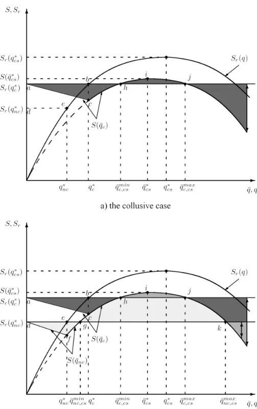
Figure 3 a) illustrates i(q) (the lower curve) and shows qnc < qc as well as i(qnc) <
i(qc) (points e and b). When the economy changes from non-cooperation to collusion,
prices in the remanufacturing sector (equations 2 and 3) strictly decrease while the market share of good quality products increases. Therefore, collusion bene…ts not only producers but also consumers. This result recalls Carlton and Waldman (2009) where the monopolist on the original market is also the low-cost remanufacturer. Comparing with the competitive case, monopolizing the remanufacturing market increases welfare since used products are remanufactured in the lowest cost manner. In their model however, the monopolist captures all the bene…ts and the consumer surplus stays unchanged.
Proposition 1 suggests that a government could substitute environmental regulations by legislating industrial agreements on the level of remanufacturability. The parallel can be made with the National Cooperative Research Act of 1984, in the US, which promotes col-lusion on innovation and R&D. Extended producer responsibility, a new type of regulation
where producers are responsible for their end-of-life product management,19 also o¤ers
plat-forms where certain kinds of collusions are encouraged. In the alternator industry, these agreements could take place within manufacturers and remanufacturers associations like the international Automotive Parts Remanufacturers Association or the United States Council
for Automotive Research.20
19See for instance the EU Waste Electrical and Electronic Equipment (WEEE) Directive. 20See http://apra.org/ and www.uscar.org.
4
Environmental regulation
In this economy, the government may decide to introduce an environmental regulation which establishes a minimum level of remanufacturability, denoted by q.
Here, the objective is not to solve for the social planner’s problem, but to observe how the industry would react in case of an environmental regulation. In particular, the analysis shows under which conditions the OMs go along with the regulation or resist compliance with it.
4.1
Public intervention
Under public intervention, the four stages stay the same but …rms face a more stringent
technological constraint: qi q. Because this regulation applies also to the outsider, the
minimum production cost increases at cm(q) and the second stage equilibrium leads to an
increased original component’s price:
pm1= pm2 = cm(q):
Hence, the pro…t function becomes:
i(qk) = (cm(q) cm(qk)) 1 2 + b X t=1 t l ri(qk) 2 (15)
where i and qkdesignate the pro…t and the optimal level of remanufacturability under
envi-ronmental regulations. With k 2 fnc; cg, equation (15) stands for either the non-cooperative or the collusive case and respects the equilibrium condition which stays equation (11) or (13). An environmental regulation will be e¤ective if it is larger than voluntary
remanufactura-bility, i.e. when q > qk. However, if a regulation applies to di¤erent industries with uneven
q < qk. In this case, the regulation constraint is not biding and the selected level of reman-ufacturability stays unchanged. The applied level of remanreman-ufacturability and the di¤erence in pro…ts before and after regulation are:
qk = 8 < : qk if qk q q if qk q (16) i(qk) i(qk) = 8 > > < > > : (cm(q) cm(0)) 2 if qk q (cm(qk) cm(0)) 2 + b X t=1 t l[ (ri(q)2 ri(qk)2)]if qk q (17)
Figure 3 a) shows how pro…ts vary with the imposition of a regulation in the collusive case. Figure 3 b) combines both the collusive and the non-cooperative cases. The vertical
distance between the curves i(qk)and the horizontal lines i(qk)describes the di¤erence in
pro…ts due to all possible levels of regulation. The light and medium shade areas show the non-cooperative case while the medium and dark shade areas exhibit the collusive case.
When the regulation is non-e¤ective (i.e. when qk = qk q), the level of
remanufactura-bility stays unchanged. However, the OMs’pro…t increases by (cm(q) cm(0))=2due to the
higher original product price. For the collusive (non-cooperative) case, this corresponds to the vertical distance in the triangle abc (def).
An e¤ective regulation (qk = q > qk) in‡uences OMs’pro…ts through two e¤ects. First,
price and cost are now equal on the primary market and OMs’initial de…cit vanishes. This
shifts up pro…ts by (cm(qk) cm(0))=2. For the collusive (non-cooperative) case, this is
the vertical distance bc (ef). Second, a higher level of remanufacturability in‡uences OMs’ technological advantage and, consequently, their ability to reach a larger aftermarket share
(equations 9 and 10). As long as the OMs gain technological advantage, c0
s(q) c0r(q) 0,
their pro…ts increase. When c0s(q) c0r(q) 0, the technological gap lessens and OMs see
their aftermarket share reduced. Thereafter, the pro…t under regulation decreases until it
reaches the initial …rm’s pro…t i(qk) at q = q
max
overtakes the …rst one. Above this threshold, regulation results in net costs for the OMs. Total variation following an e¤ective regulation is represented by bcg (efcgh) and the shaded area beyond gh (h).
Proposition 2 Environmental regulations can increase …rms’bene…ts in both the non-cooperative
and the collusive cases:
i(qk) i(qk) > 0 () q < qmaxk :
In particular, this remains true when the environmental regulation is e¤ective:
i(qk) i(qk) > 0 () qk q < q
max k
This result coincides with the Porter Hypothesis, which says that pro…ts may increase in the industry with the application of environmental regulations. The present model corrobo-rates the argument of Ambec and Barla (2007) under which the Porter Hypothesis requires the presence of at least one market imperfection beside the environmental externality. The phenomenon is here the result of two market characteristics.
The …rst is the threat of the outsider on the primary market, which keeps the original price at the minimum production cost. Hence, OMs cannot pass on the information through prices that a product is remanufacturable. The competitive …nal good producers do not bene…t from remanufacturability and see no incentive in raising production costs. Therefore,
the selling price stays pm = cm(0). When the regulation takes place, the selling price pm
carries the information up to the point justi…ed by the public intervention (pm = cm(q)).
This result shows how free-entry on the original alternator market has prevented OMs from engaging in remanufacturing initiatives and how the asbestos ban was welcomed by the industry.
is known that collusion leads to higher pro…ts. Here, the regulation solves for this collective action problem. Although non-cooperation is not a necessary condition in con…rming the Porter Hypothesis, it increases the extent to which regulations generate pro…ts. This speci…c e¤ect is graphically represented in Figure 3 by the area framed above and below by the
horizontal lines i(qc)and i(qnc), and to the left by eb. André et al. (2009) obtains similar
results when a duopoly simultaneously choose between the production of a "standard" or a "green" product. A discrete choice of options can keep the standard quality as the Nash equilibrium, even if Pareto dominated by the green choice. Therefore, a regulation that forces cooperation between …rms for the environmentally-friendly option can bene…t …rms, consumers and the environment. This additional role given to the regulation explains the di¤erence between the non-cooperative and the collusive scenarios and leads to propositions 3 and 4.
In view of the positive variation in pro…ts, any regulation below qmax
k should be positively
supported by the OMs. In contrast, regulations above qmax
k are likely to meet resistance in
their application. The di¤erence in pro…ts before and after the regulation (equation 17) can therefore be interpreted as the intensity of compliance or resistance towards the regulation. Hence:
Proposition 3 It is always easier to introduce an environmental regulation q under the
non-cooperative case:
i(qnc) i(qnc) > i(qc) i(qc)
Proposition 4 The maximum level of regulation positively supported by the industry is
larger under the non-cooperative case:
In the absence of environmental regulation, the government can promote collusion as a substitute for regulation. However, when a regulation is scheduled, collusion should be repressed since non-cooperation better supports the regulation.
4.2
Intervention maximizing OMs’pro…t
Let q denotes the optimal regulation that would be chosen by the OMs. This scenario di¤ers from the collusive case in the absence of regulation; for whichever level of remanufacturability chosen by the OMs, the outsider, constrained by the regulation, will not have the opportunity
to produce at lower costs and, consequently, the threat vanishes. With pm1 = pm2= cm(q),
the maximization problem is:
max q 0 i = b X t=1 t l[ ri(q) 2] s.t. ri(q) = + cs(q) cr(q) 3 .
The optimal condition is:
@ i
@q = 0 () c
0
s(q ) c0r(q ) = 0 (18)
and the second-order condition is always satis…ed. Note that q coincides with q, the levelb
of remanufacturability that maximizes the OMs’technological advantage (see equation 10).
Figure 3 displays q and i(q ), the privately optimal regulation and the corresponding
pro…t. Comparing the optimal conditions for the determination of q , qc and qnc leads to
the following propositions:
remanufac-turability above the one chosen in absence of regulation:
q > qc > qnc
Proof: From Proposition 1, it is already known that qc > qnc. The optimal conditions
(11) and (13) for the choice of q in absence of environmental regulation imply a positive value of (c0
s(q) c0r(q)): Since c00s(q) c00r(q) < 0 in this neighbourhood (equation 10), it is
straightforward to see that the condition leading to the private optimal choice of regulation (18) results in q > qc > qnc.
Proposition 6 The size of remanufacturing activities (for the OMs) is maximized if and
only if the public sector …xes the regulation at the level preferred by the OMs: @ri
@q =
(c0
s(q) c0r(q))
3 = 0() q = q
When the regulation is selected by the private sector, OMs take into account the fact that the entire production cost is covered by the selling price. They can therefore seize the maximum aftermarket share by costlessly choosing the level of remanufacturability leading to their largest technological advantage. When q = q , OMs’s pro…ts are maximized as well as their aftermarket size.
When OMs’ remanufacturing activities pollute signi…cantly less than IRs’, the social planner may want to maximize the OMs’ aftermarket share to the detriment of higher re-manufacturability by choosing q = q .
4.3
Welfare analysis
On the inelastic original market, consumer surplus varies only with the price. Hence, in
equilibrium, it can be de…ned as Sm = Sm(pm) = Sm(cm(q)) where Sm(a) Sm(b) =
the remanufacturing market, Sr(q) (equation 14), total consumer surplus in the presence of a regulation becomes: S(qk) = Sm(q) + Xb t=1 t l 2 (1 ) + ri(qk) 2+ 2( c s(qk)) :
The change in consumer surplus following an environmental regulation is de…ned by:
S(qk) Sr(qk) = 8 > > > < > > > : (cm(q) cm(0)) if qk q (cm(q) cm(0))+ Xb t=1 t l 2 [ (ri(q)2 ri(qk)2) 2(cs(q) cs(qk))] if qk q (19)
Figure 4 a) illustrates a particular case of equation (19) in the collusive scenario. Figure 4 b) combines both the collusive and the non-cooperative cases. The upper curve is the consumer surplus with respect to the level of remanufacturability in the absence of regulation.
The horizontal line Sr(qc) (respectively Sr(qnc)) is the consumer surplus in the collusive
(non-cooperative) case where, following Proposition 1, Sr(qc) > Sr(qnc). In the presence of
regulation, the lower curve shows the consumer surplus if the industry were to adopt exactly
q, however for low levels of regulation, the industry keeps producing at qk. The vertical
distance between the curves S(qk) and Sr(qk) describes the di¤erence in consumer surplus
due to all possible level of regulation. The medium and dark (light and medium) shade areas exhibit the collusive (non-cooperative) case.
When the regulation is non-e¤ective (i.e. for qk q), the level of remanufacturability
stays …xed but the price increases on the original market. Consumer surplus is therefore
reduced by (cm(q) cm(0)), illustrated in the triangle abc (def).
Proposition 7 A non-e¤ective environmental regulation lets the social welfare that equally
weights total pro…ts and consumer surplus unchanged.
A non-e¤ective regulation partially shifts the cost of remanufacturability from OMs to-wards …nal good producers and consumers. This can be seen using equations (17) and (19) expressing the change in pro…t and the change in consumer surplus. Considering the environ-mental neutrality of non-e¤ective regulations, this money transfer leaves the social welfare unchanged.
When the regulation is e¤ective, it can be shown that for some speci…c scenarios, a variation in the level of remanufacturability reduces prices of remanufactured products and increases the share of high quality goods on the aftermarket so that the net variation in
consumer surplus is positive. Let qcs be the e¤ective environmental regulation that locally
maximizes consumer surplus. The subscript cs designates consumer surplus. The constraints for a maximum are:
c0m(qcs) + b X t=1 t l (c0 s(qcs) c0r(qcs)) 3 ri(qcs) c 0 s(qcs) = 0: c00m(qcs) + b X t=1 t l " (c00 s(qcs) c00r(qcs)) 3 ri(qcs) + (c0 s(qcs) c0r(qcs)) 3 2 c00s(qcs) # 0
Comparing with the optimality conditions for the choice of qnc and qc (equations 11 and 13),
there exists (at least) one local maximum for the function (19) only if qcs qk, which occurs
when the decreasing remanufacturing cost c0
s is large enough compared to the increasing
original production cost c0m, when evaluated at qk.
21 Otherwise, consumer surplus strictly
decreases with more stringent regulation. The regulation can be welfare improving for the
consumer only if S(qcs) S(qk), in which case the net positive variation in consumer surplus
is illustrated by the area hij (ghijk) for the collusive (non-cooperative) case. When the regulation becomes too stringent, the market share of high quality remanufactured products
drops, which causes the consumer surplus to decrease. At qmax
k;cs (beyond j (k)), the regulation
21Note that, under certain conditions, the consumer surplus function in the presence of regulation allows
for multiple maxima for q qk. For simplicity, the following results are presented for cases where there is at most one maximum.
is a net cost for the consumer. This leads to the following propositions:
Proposition 8 When S(qcs) S(qk), an e¤ective environmental regulation can increase
consumer surplus:
S(q) Sr(qk) 0 if qmink;cs q qmaxk;cs
More particularly, when S(qcs) S(qk) and qmin
k;cs qmaxk , an e¤ective environmental
regula-tion can increase both pro…ts and consumer surplus:
i(qk) i(qk) 0 and S(q) Sr(qk) 0 if q min k;cs q minfq max k;cs; q max k g
Under some circumstances, the government can apply an environmental regulation for which, in addition to environmental advantages, producers and consumers bene…t from higher pro…ts and lower prices.
Proposition 9 It is always easier to introduce an e¤ective environmental regulation under
the non-cooperative case:
S(qnc) Sr(qnc) < S(qc) Sr(qc)
Proposition 10 When S(qcs) S(qk) for k = c; nc, the range of regulations positively
supported by consumers is larger under the non-cooperative case:
qmaxnc;cs qminnc;cs> qmaxc;cs qminc;cs:
This stays true when S(qcs) S(qnc) and S(qcs) S(qc) since
Propositions 9 and 10 say that, when the di¤erence in consumer surplus before and after the regulation is interpreted as the intensity of political support for the regulation, the government should repress collusion. These results are in line with Propositions 3 and 4 where …rms are more likely to comply with the public intervention when they compete on the level of remanufacturability.
5
Conclusion
Original manufacturers produce a component as an input for the …nal good where the threat of an outsider keeps the input’s price at the minimum production cost. At the same time, they select the technology determining the level of remanufacturability of their products. Later, consumers of the …nal good have to replace the speci…c component. They consider products remanufactured by either independent remanufacturers or original manufacturers, and they are willing to pay a price premium for the latter. In this set-up, used products can be remanufactured by any …rms, causing original manufacturers to su¤er from free-riding on their technology selection and discouraging investment in remanufacturing-oriented designs. When the original manufacturers collude on the level of remanufacturability, they only face the externality of independent remanufacturers and select a higher level of remanufactura-bility. Collusion bene…ts producers and, by reducing prices on the aftermarket, consumers.
Remanufacturing bene…ts the population through less post-consumption waste, lower en-ergy and raw material consumptions, and lower prices for replacement products. It can also bene…t the industry through the generation of positive pro…ts. While the gains of remanu-facturing are shared among the society, the costs of remanuremanu-facturing-oriented technology are born solely by the original manufacturers. Consequently, public regulation may be necessary. The introduction of an environmental regulation, which imposes a minimal level of reman-ufacturability, justi…es a price increase on the primary market. As a consequence, the cost
of complying with the regulation is redirected towards …nal good producers and consumers. Hence, original manufacturers can see their pro…ts increase. This observation corroborates the Porter Hypothesis. Under some circumstances, the environmental regulation can also increase consumer surplus.
A social planner who wants to stimulate remanufacturing activities can consider allowing private collusion as an alternative to environmental regulation since it leads to a higher level of remanufacturability. Moreover, collusion leads to a larger supply of high quality reman-ufactured products and to lower prices on the aftermarket and, hence, increases consumer surplus. The application of an environmental regulation reduces the threat of the outsider and solves for the collective action problem. If the social planner opts for this option, it should repress private collusions. When the variation in pro…ts following the public inter-vention is interpreted as the industrial degree of cooperation with the regulation, original manufacturers will always o¤er stronger support, or lower opposition, when the technology choice is initially subject to free-riding.
References
Ambec, Stefan, and Philippe Barla (2007) ‘Survol des fondements théoriques de l’hypothèse de Porter.’L’Actualité économique 83, 399–413
André, Francisco J., Paula González, and Nicolás Porteiro (2009) ‘Strategic quality competi-tion and the Porter Hypothesis.’Journal of Environmental Economics and Management 57, 182–194
Canton, Joan (2008) ‘Redealing the cards: How an eco-industry modi…es the political econ-omy of environmental taxes.’Resource and Energy Economics 30, 295–315
Carlton, Dennis W., and Michael Waldman (2009) ‘Competition, monopoly, and aftermar-kets.’The Journal of Law, Economics, & Organization 26, 54–91
Cellini, Roberto, and Luca Lambertini (2009) ‘Dynamic R&D with spillovers: Competition vs cooperation.’Journal of Economic Dynamics & Control 33, 568–582
Chung, Chun-Jen, and Hui-Ming Wee (2008) ‘Green-component life-cycle value on design and reverse manufacturing in semi-closed supply chain.’International Journal of Production Economics 113, 528–545
D’Aspremont, Claude, and Alexis Jacquemin (1988) ‘Cooperative and noncooperative R&D in duopoly with spillovers.’The American Economic Review 78, 1133–1137
David, Maia, and Bernard Sinclair-Desgagné (2005) ‘Environmental regulation and the eco-industry.’Journal of Regulatory Economics 28, 141–155
Debo, Laurens G., L. Beril Toktay, and Luk N. Van Wassenhove (2005) ‘Market segmentation and product technology selection for remanufacturable products.’Management Science 51, 1193–1205
Eichner, Thomas, and Marco Runkel (2005) ‘E¢ cient policies for green design in a vintage durable good model.’Environmental and Resource Economics (2005) 30, 259–278 Eichner, Thomas, and Rudiger Pethig (2001) ‘Product design and e¢ cient management of
recycling and waste treatment.’Journal of Environmental Economics and Management 41, 109–134
European Commission (1999) ‘Commission directive 1999/77/EC.’ O¢ cial Journal of the European Communities L207, 18
Ferrer, Geraldo (1997) ‘The economics of personnal computer remanufacturing.’Resources, Conservation and Recycling 21, 79–108
(2000) ‘Market segmentation and product line design in remanufacturing.’Technical Re-port, Working paper, The Kenan-Flagler Business School, University of North Carolina, Chapel Hill, NC.
Ferrer, Geraldo, and Jayashankar M. Swaminathan (2006) ‘Managing new and remanufac-tured products.’Management Science 52, 15–26
Fullerton, Don, and Wenbo Wu (1998) ‘Policies for green design.’Journal of Environmental Economics and Management 36, 131–148
Giuntini, Ron, and Kevin Gaudette (2003) ‘Remanufacturing: The next great opportunity for boosting US productivity.’Business Horizons 46, 41–48
Goel, Rajeev K. (1990) ‘Innovation, market structure, and welfare: a Stackelberg model.’ Quarterly Review of Economics and Business 30, 40–53
Heese, Hans S., Kyle Cattani, Geraldo Ferrer, Wendell Gilland, and Aleda V. Roth (2005) ‘Competitive advantage through take-back of used products.’European Journal of Op-erational Research 164, 143–157
Kiesmuller, Gudrun P., and Erwin A. van der Laan (2001) ‘An inventory model with de-pendent product demands and returns.’International Journal of Production Economics 72, 73–87
Kim, Hyung-Ju, Semih Severengiz, Steven J. Skerlos, and Gunther Seliger (2008) ‘Economic and environmental assessment of remanufacturing in the automotive industry’
Klemperer, Paul (1995) ‘Competition when consumers have switching costs: An overview with applications to industrial organization, macroeconomics, and international trade.’ Review of Economic Studies 62, 515–539
Lebreton, Baptiste, and Axel Tuma (2006) ‘A quantitative approach to assessing the prof-itability of car and truck tire remanufacturing.’ International Journal of Production Economics 104, 639–652
Majumder, Pranab, and Harry Groenevelt (2001) ‘Competition in remanufacturing.’ Pro-duction and Operations Management 10, 125–141
Mitra, Supriya, and Scott Webster (2008) ‘Competition in remanufacturing and the e¤ects of government subsidies.’International Journal of Production Economics 111, 287–298 Organization for Economic Cooperation and Development/Eurostat (1999) The Environ-mental and Services Industry: Manual for Data Collection and Analysis (Paris: OECD) Steinhilper, Rolf (1998) Remanufacturing The Ultimate Form of Recycling (Remanufacturing
Industries Council International Automotive Parts Rebuilders Association (APRA)) To¤el, Michael W. (2004) ‘Strategic management of product recovery.’California
Manage-ment Review 46, 120–141
To¤el, Michael W., Antoinette Stein, and Katharine L. Lee (2008) ‘Extending producer re-sponsibility: An evaluation framework for product take-back policies.’Technical Report, Harvard Business School
Webster, Scott, and Supriya Mitra (2007) ‘Competitive strategy in remanufacturing and the impact of take-back laws.’Journal of Operations Management 25, 1123–1140