HAL Id: hal-00375232
https://hal.archives-ouvertes.fr/hal-00375232v2
Submitted on 9 Jun 2009
HAL is a multi-disciplinary open access
archive for the deposit and dissemination of sci-entific research documents, whether they are pub-lished or not. The documents may come from teaching and research institutions in France or
L’archive ouverte pluridisciplinaire HAL, est destinée au dépôt et à la diffusion de documents scientifiques de niveau recherche, publiés ou non, émanant des établissements d’enseignement et de recherche français ou étrangers, des laboratoires
On stratified regions
Roberto M. Amadio
To cite this version:
Roberto M. Amadio. On stratified regions. Proceedings of the 7th Asian Symposium on Programming Languages and Systems, Dec 2009, South Korea. pp.210-225. �hal-00375232v2�
On stratified regions
Roberto M. AmadioUniversit´e Paris Diderot (Paris 7)∗
June 9, 2009
Abstract
Type and effect systems are a tool to analyse statically the behaviour of programs with effects. We present a proof based on the so called reducibility candidates that a suitable stratification of the type and effect system entails the termination of the typable programs. The proof technique covers a simply typed, multi-threaded, call-by-value lambda-calculus, equipped with a variety of scheduling (preemptive, cooperative) and interaction mecha-nisms (references, channels, signals).
Keywords Types and effects. Termination. Reducibility candidates.
1
Introduction
In the framework of functional programs, the relationship between type systems and termi-nation has been extensively studied through the Curry-Howard correspondence. It would be interesting to extend these techniques to programs with effects. By effect we mean the possibility of executing operations that modify the state of a system such as reading/writing a reference or sending/receiving a message.
Usual type systems as available, e.g., in various dialects of the ML programming language, are too poor to account for the behaviour of programs with effects. A better approximation is possible if one abstracts the state of a system in a certain number of regions and if the types account for the way programs act on such regions. So-called type and effect systems [8] are an interesting formalisation of this idea and have been successfully used to analyse stati-cally the problem of heap-memory deallocation [10]. On the other hand, the proof-theoretic foundations of such systems are largely unexplored. Only recently, it has been shown [3] that a stratification of the regions entails termination in a certain higher-order language with cooperative threads and references. Our purpose here is to revisit this result trying to clarify and extend both its scope and its proof technique (a more technical comparison is delayed to section 4). We refer to [3] for a tentative list of papers referring to a notion of stratification for programs with side effects. Perhaps the closest works in spirit are those that have adapted the reducibility candidates techniques to the π-calculus [11, 9]. Those works exhibit type systems for the π-calculus that guarantee the termination of the usual continuation passing style translations of typed functional languages into the π-calculus. However, as pointed out by one of the authors of op.cit in [5], they are not very successful in handling state sensitive programs. The approach here is a bit different: one starts with a higher-order typed func-tional language which is known to be terminating and then one determines to what extent
side-effects can be added while preserving termination. Yet in another direction, we notice that a notion of region stratification has been used in [2] to guarantee the polynomial time reactivity of a first-order timed/synchronous language.
We outline the contents of the paper. In section 2, we introduce a λ-calculus with regions. Regions are an abstraction of dynamically generated values such as references, channels, and signals, and the reduction rules of the calculus are given in such a way that the reduction rules for references, channels, and signals can be simulated by those given for regions. In section 3, we describe a simple type and effect system along the lines of [8]. In this discipline, types carry information on the regions on which the evaluated expressions may read or write. The discipline allows to write in a region r values that have an effect on the region r itself. In turn, this allows to simulate recursive definitions and thus to produce non terminating behaviours. In section 4, following [3], we describe a stratification of the regions. The idea is that regions are ordered and that a value written in a region may only produce effects in smaller regions. We then propose a new reducibility candidates interpretation (see, e.g., [6] for a good survey) entailing the termination of typable programs. In section 5, we enrich the language with the possibility to generate new threads and to react to the termination of the computation. The language we consider is then timed/synchronous in the sense that a computation is regarded as a possibly infinite sequence of instants. An instant ends when the calculus cannot progress anymore (cf. timed/synchronous languages such as Timed CCS [7] and Esterel [4]). We extend the stratified typing rules to this language and show by means of a translation into the core language that typable programs terminate. We also show that a fixed-point combinator can be defined and typed so that recursive calls are allowed as long as they arise at a later instant. This differs from [3] where a fixed-point combinator is added to the language potentially compromising the termination property. Appendix A contains the main proofs and appendix B summarizes the type and effect systems considered.
2
A λ-calculus with regions
We consider a λ-calculus with regions. Regions are abstractions of dynamically generated ‘pointers’ which, depending on the context, are called references, channels, or signals. Given a program with operators to generate dynamically values (such as ref in the ML language or ν in the π-calculus), one may simply introduce a distinct region for every occurrence of such operators. This amounts to collapse all the ‘pointers’ generated by the operator at run time into one constant. The resulting language simulates the original one as long as the values written into regions do not erase those already there. In particular, termination for the language with regions entails termination for the original language.
We notice that ordinary type system for programs with dynamic values perform a similar abstraction: all the values that are generated by an operator are assigned the same type. For instance, typing νx P in the π-calculus will reduce to typing the process P in a context where the name x is associated with a suitable type A. In the corresponding language with regions, one will replace the name x with a region r and type [r/x]P ([r/x] is the substitution) in a region context where r is associated with A.
To summarise, termination for the language with regions entails termination for the orig-inal calculi and moreover ordinary type system implicitly abstract dynamically generated values into regions. Therefore, we argue that one can carry on the main type theoretic argu-ments at the level of regions rather than at the more detailed level of dynamically generated
values. 1
2.1 Syntax
We consider the following syntactic categories:
x, y, . . . (variables)
r, s, . . . (regions)
e, e′, . . . (finite sets of regions)
A ::= 1 || RegrA || (A −→ A)e (types) Γ ::= x1 : A1, . . . , xn: An (context)
R ::= r1: A1, . . . , rn: An (region context)
M ::= x || r || ∗ || λx.M || M M || get(M ) || set(M, M ) (terms)
V ::= r || ∗ || λx.M (values)
v, v′, . . . (sets of value)
S ::= (r ⇐ v) || S, S (stores)
X ::= M || S (stores or terms)
P ::= X || X, P (programs)
We briefly comment the notation: 1 is the terminal (unit) type with value ∗; RegrA is the type of a region r containing values of type A; A −→ B is the type of functions that whene given a value of type A may produce a value of type B and an effect on the regions in e; get is the operator to read some value in a region and set is the operator to insert a value in a region.
We write [N/x]M for the substitution of N for x in M . If R = r1 : A1, . . . , rn : An then
dom(R) = {r1, . . . , rn}. If r ∈ dom(R) then we write R(r) for the type A such that r : A
occurs in R. We also define the term regrM as an abbreviation for (λx.r)(set(r, M )). Thus the difference between set(r, M ) and regrM is that in the first case we return ∗ while in the second we return r. When writing a program P = X1, . . . , Xn we regard the symbol ‘,’ as
associative and commutative, or equivalently we regard a program as a multi-set of terms and stores. We write (r ⇐ V ) for (r ⇐ {V }). We shall identify the store (r ⇐ v1), (r ⇐ v2) with
the store (r ⇐ v1∪ v2). We denote with dom(S) the set of regions r such that (r ⇐ v) occurs
in S and define S(r) as the set {V | (r ⇐ V ) occurs in S}. 2.2 Reduction
A call-by value evaluation context E is defined as:
E ::= [ ] || EM || V E || get(E) || set(E, M ) || set(V, E) An elementary evaluation context is defined as:
El ::= [ ]M || V [ ] || get([ ]) || set([ ], M ) || set(V, [ ]) 1
Incidentally, it seems much easier to produce denotational models of languages with regions than for the original languages with dynamic values so that one can hope to find models that do provide insight into the type systems.
An evaluation context can be regarded as the finite composition (possibly empty) of elemen-tary evaluation contexts. The reduction on programs is defined as follows:
E[(λx.M )V ] → E[[V /x]M ] E[get(r)], (r ⇐ V ) → E[V ], (r ⇐ V )
E[set(r, V )] → E[∗], (r ⇐ V )
P → P′ P, P′′→ P′, P′′
Note that the semantics of set amounts to add rather than to update a binding between a region and a value. Hence a region can be bound at the same time to several values (possibly infinitely many) and the semantics of get amounts to select non-deterministically one of them. As already mentioned, the notion of region is intended to simulate some familiar pro-gramming concepts such as references, channels, or signals. Specifically: (i) when writing a reference, we replace the previously written value (if any), (ii) when reading a (unordered, unbounded) channel we consume (remove from the store) the value read, and finally (iii) the values written in a signal persist within an instant and disappear at the end of it.2 One
can easily formalise the reduction rules for references, channels, and signals, and check that (within an instant) each reduction step is simulated by at least one reduction step in the cal-culus with regions. Thus, typing disciplines that guarantee termination for the calcal-culus with regions will guarantee the same property when adapted to references, channels, or signals.
3
Types and effects: unstratified case
We introduce a simple type and effect system along the lines of [8]. The following rules define when a region context R is compatible with a type A (judgement R ↓ A):
R ↓ 1
R ↓ A R ↓ B e ⊆ dom(R) R ↓ (A−→ B)e
r : A ∈ R R ↓ RegrA
The compatibility relation is just introduced to define when a region context is well formed (judgement R ⊢) and when a type and effect is well-formed with respect to a region context (judgements R ⊢ A and R ⊢ (A, e)).
∀ r ∈ dom(R) R ↓ R(r) R ⊢ R ⊢ R ↓ A R ⊢ A R ⊢ A e ⊆ dom(R) R ⊢ (A, e)
A more informal way to express the condition is to say that a judgement r1: A1, . . . , rn: An⊢
B is well formed provided that: (1) all the region names occurring in the types A1, . . . , An, B
belong to the set {r1, . . . , rn} and (2) all types of the shape RegriC with i ∈ {1, . . . , n} and
occurring in the types A1, . . . , An, B are such that C = Ai. For instance, the reader may verify
that r : 1 −−→ 1 ⊢ Reg{r} r1 {r}
−−→ 1 can be derived while r1 : Regr2(1
{r2}
−−→ 1), r2 : 1 {r1}
−−→ 1 ⊢ cannot. Also it can be easily checked that the following properties hold:
R ⊢ 1 iff R ⊢
R ⊢ RegrA iff R ⊢ and R(r) = A
R ⊢ A−→ B iff R ⊢, R ⊢ A, R ⊢ B, and e ⊆ dom(R)e R ⊢ iff ∀ r ∈ dom(R) R ⊢ R(r)
2
The subset relation on effects induces a subtyping relation on types and on pairs of types and effects which is defined as follows (judgements R ⊢ A ≤ A′, R ⊢ (A, e) ≤ (A′, e′)):
R ⊢ A R ⊢ A ≤ A R ⊢ A′ ≤ A R ⊢ B ≤ B′ e ⊆ e′⊆ dom(R) R ⊢ (A−→ B) ≤ (Ae ′ e−→ B′ ′) R ⊢ A ≤ A′ e ⊆ e′ ⊆ dom(R) R ⊢ (A, e) ≤ (A′, e′) We notice that the transitivity rule:
R ⊢ A ≤ B R ⊢ B ≤ C R ⊢ A ≤ C
can be derived via a simple induction on the height of the proofs. The subtyping rule trades flexibility against precision of the type system. For instance, suppose A1 = 1 e
1
−→ 1 and A2 = 1
e2
−→ 1 and we want to define the type B of the functionals that take a value V1 of
type A1 and a value V2 of type A2 and compute either V1∗ or V2∗. We can define B =
A1 −→ (A∅ 2 e1∪e2
−−−→ 1). The reader can check that both λx.λy.x∗ and λx.λy.y∗ have type B provided the subtyping rule is used. Incidentally, we note that [3] seems to ‘forget’ the subtyping rule. While there are is no particular problems to provide a reducibility candidates interpretation for this rule, we notice that without it the following diverging ML expression let l = ref(λx.x) in l := λx.!lx; !l(), which is given in op.cit. to motivate the stratification of regions does not type already in the ordinary unstratified type and effect system because (λx.x) has type 1−→ 1 but not 1∅ −−→ 1 where r is the region associated with the reference l.{r} We now turn to the typing rules for the terms. We shall write R ⊢ x1 : A1, . . . , x : An if
R ⊢ and R ⊢ Ai for i = 1, . . . , n. Note that in the following rules we always refer to the same
region context R. R ⊢ Γ x : A ∈ Γ R; Γ ⊢ x : (A, ∅) R ⊢ Γ r : A ∈ R R; Γ ⊢ r : (RegrA, ∅) R ⊢ Γ R; Γ ⊢ ∗ : (1, ∅) R; Γ, x : A ⊢ M : (B, e) R; Γ ⊢ λx.M : (A−→ B, ∅)e R; Γ ⊢ M : (A e2 −→ B, e1) R; Γ ⊢ N : (A, e3) R; Γ ⊢ M N : (B, e1∪ e2∪ e3) R; Γ ⊢ M : (RegrA, e) R; Γ ⊢ get(M ) : (A, e ∪ {r}) R; Γ ⊢ M : (RegrA, e1) R; Γ ⊢ N : (A, e2) R; Γ ⊢ set(M, N ) : (1, e1∪ e2∪ {r}) R; Γ ⊢ M : (A, e) R ⊢ (A, e) ≤ (A′, e′) R; Γ ⊢ M : (A′, e′)
Finally, we extend the typing rules to stores and general multi-threaded programs. To this end, it is convenient to introduce a constant behaviour type B which is the type we give to multi-sets of threads and/or stores which are not supposed to return a value but just to interact via side-effects. We will use α, α′, . . . to denote either an ordinary type A or this new behaviour type B.
r : A ∈ R ∀ V ∈ v R; Γ ⊢ V : (A, ∅) R; Γ ⊢ (r ⇐ v) : (B, ∅)
R; Γ ⊢ Xi : (αi, ei) i = 1, . . . , n ≥ 1
Remark 1 The derived typing rule for regrM is as follows:
r : A ∈ R R; Γ ⊢ M : (A, e) R; Γ ⊢ regrM : (RegrA, e ∪ {r})
One can derive a more traditional ‘effect-free’ type system by erasing all the effects from the types and the typing judgements. Note that in the resulting system the subtyping rules are useless. We shall write ⊢ef for provability in this system. This ‘weaker’ type system
suffices to state a decomposition property of the terms which is proven by induction on the structure of the term.
Proposition 2 (decomposition) If R; ⊢ef M : A is a well-typed closed term then exactly
one of the following situations arises where E is an evaluation context:
1. M is a value.
2. M = E[∆] and ∆ has the shape (λx.N )V , set(r, V ), or get(r).
3.1 Basic properties of typing and evaluation
We observe some basic properties: (i) one can weaken both the type and region contexts, (ii) typing is preserved when we replace a variable with an effect-free term of the same type, and (iii) typing is preserved by reduction. If S is a store and e is a set of regions then S|e is the store S restricted to the regions in e.
Proposition 3 (basic properties, unstratified) The following properties hold: weakening If R; Γ ⊢ M : (A, e) and R, R′⊢ Γ, Γ′ then R, R′; Γ, Γ′⊢ M : (A, e).
substitution If R; Γ, x : A ⊢ M : (B, e) and R; Γ ⊢ N : (A, ∅) then R; Γ ⊢ [N/x]M : (B, e). subject reduction Let M denote a sequence M1, . . . , Mn. If R, R′; ⊢ M, S : (B, e), R ⊢ e,
and M, S → M′, S′ then R, R′; ⊢ M′, S′ : (B, e), S
|dom(R′) = S|dom(R′ ′), and M, S|dom(R)→
M′, S|dom(R)′ . Moreover, if M = M and R, R′ ⊢ M : (A, e) then M′ = M′ and
R, R′ ⊢ M′: (A, e).
The weakening and substitution properties are shown directly by induction on the proof height. Concerning subject reduction, it is useful to notice that if a term M , of type and effect (A, e), is ready to read/write the region r then r ∈ e. This follows from an analysis of the evaluation context. Then we prove the assertion by case analysis on the reduction rule applied, relying on the substitution property.
Remark 4 The subject reduction property is formulated so as to make clear that the type
and effect system indeed delimits the interactions a term may have with the store. Note that a term may refer to regions which are not explicitly mentioned in its type and effect. For instance, consider M = (λf.∗)(λx.get(r)x) and let R = r : 1−→ 1. Then R; ∅ ⊢ M : (1, ∅),∅ ∅ ⊢ (1, ∅) but ∅; ∅ 6⊢ M : (1, ∅). The subject reduction property guarantees that such a term
3.2 Recursion
In our (unstratified) calculus, we can write in a region r a functional value λx.M where M reads from the region r itself. For instance, regr(λx.(get(r))x).
This kind of circularity leads to diverging computations such as:
get(regrλx.get(r)x)∗ → get(r)∗, (r ⇐ λx.get(r)x) → (λx.get(r)x)∗, (r ⇐ λx.get(r)x) → get(r)∗, (r ⇐ λx.get(r)x) → · · ·
It is well known that this phenomena can be exploited to simulate recursive definitions. Specifically, we define:
fixrf.M = λx.(get(regr(λx.[λx.get(r)x/f ]M x))) x (1)
By a direct application of the typing rules and proposition 3(substitution), one can derive a rule to type fixrf.M .
Proposition 5 (type fixed-point) The following typing rule for the fixed point combinator
is derived: r : A−→ B ∈ Re r ∈ e R; Γ, f : A−→ B ⊢ M : (Ae −→ B, ∅)e R; Γ ⊢ fixrf.M : (A e − → B, ∅) (2)
For a concrete example, assume basic operators on the integer type and let M be the factorial function:
M = λx.if x = 0 then 1 else x ∗ f (x − 1) . Then compute (fixrf.M )1. In this case we have e = {r} and r : int
r
−
→ int ∈ R.
4
Types and effects: stratified case
As we have seen, an unstratified simply typed calculus with effects may produce diverging computations. To avoid this, a natural idea proposed by G. Boudol in [3] is to stratify regions. Intuitively, we fix a well-founded order on regions and we make sure that values stored in a region r can only produce effects on smaller regions. For instance, suppose V is a value with type (1−−→ 1). Intuitively, this means that when applied to an argument U : 1, V may{r} produce an effect on region {r}. Then the value V can only be stored in regions larger than r. We shall see that this stratification allows for an inductive definition of the values that can be stored in a given region.
The only change in the type system concerns the judgements R ⊢, R ⊢ A, and R ⊢ (A, e) whose rules are redefined as follows:
∅ ⊢ R ⊢ A r /∈ dom(R) R, r : A ⊢ R ⊢ R ⊢ 1 R ⊢ r : A ∈ R R ⊢ RegrA R ⊢ A R ⊢ B e ⊆ dom(R) R ⊢ A−→ Be R ⊢ A e ⊆ dom(R) R ⊢ (A, e) .
Proviso Henceforth we shall use ⊢ to refer to provability in the stratified system and ⊢u for provability in the unstratified one. The former implies the latter since R ⊢ implies R ⊢u
and R ⊢ A implies R ⊢u A, while the other rules are unchanged.
4.1 Basic properties revisited
The main properties we have proven for the unstratified system can be specialised to the stratified one.
Proposition 6 (basic properties, stratified) The following properties hold in the
strati-fied system.
weakening If R; Γ ⊢ M : (A, e) and R, R′⊢ Γ, Γ′ then R, R′; Γ, Γ′⊢ M : (A, e).
substitution If R; Γ, x : A ⊢ M : (B, e) and R; Γ ⊢ N : (A, ∅) then R; Γ ⊢ [N/x]M : (B, e). subject reduction If R, R′; ⊢ M, S : (B, e), R ⊢ e, and M, S → M′, S′ then R, R′; ⊢
M′, S′ : (B, e), S|dom(R′) = S|dom(R′ ′), and M, S|dom(R) → M′, S|dom(R)′ . Moreover, if
M = M and R, R′; ⊢ M : (A, e) then M′ = M′ and R, R′; ⊢ M′: (A, e).
4.2 Interpretation
We describe a reducibility candidates interpretation that entails that typed programs termi-nate. We denote with SN the collection of strongly normalising single-threaded programs,
i.e., the programs of the shape M, S such that all reduction sequences terminate. We write
(M, S) ⇓ (N, S′) if M, S −→ N, S∗ ′ and N, S′ 6→. We write R′ ≥ R, and say that R′ extends R, if R′ ⊢ and R′= R, R′′ for some R′′.
The starting idea is that the interpretation of R ⊢ is a set of stores and the interpretation of R ⊢ (A, e) is a set of terms. One difficulty is that the stores and the terms may depend on a region context R′ which extends R. We get around this problem, by making the context R′ explicit in the interpretation. Then the interpretation can be given directly by induction on the provability of the judgements R ⊢ and R ⊢ (A, e). This is a notable simplification with respect to the approach taken in [3] where a rather ad hoc well-founded order on judgements is introduced to define the interpretation.
A second characteristic of our approach is that the properties a thread must satisfy are specified with respect to a ‘saturated’ store which intuitively already contains all the values the thread may write into it. This approach simplifies the interpretation and provides a simple argument to extend the termination argument from single-threaded to multi-threaded programs. Indeed, if we a have a set of threads which are guaranteed to terminate with respect to a saturated store then their parallel composition will terminate too. To see this, one can reason by contradiction: if the parallel composition diverges then one thread must run infinitely often and, since the threads cannot modify the saturated store (what they write is already there), this contradicts the hypothesis that all the threads taken alone with the saturated store terminate.
Finally, minor technical differences with respect to [3] is that we interpret the subtyping rule (cf. discussion in section 3) and that our notion of reducibility candidate follows Girard rather than Stenlund-Tait (see [6] for a detailed comparison and references).
Region-context Let R = r1 : A1, . . . , rn : An and Rri = r1 : A1, . . . , ri−1 : Ai−1, for
i = 1, . . . , n. We interpret a region-context R as a set of pairs R′ ⊢ S where R′ is a
region-context which extends R and S is a ‘saturated’ store whose domain coincides with R:
R = { R′⊢ S | R′ ≥ R, dom(S) = dom(R), and for i = 1, . . . , n
S(ri) = {V | R′ ⊢ V ∈ Rri ⊢ (Ai, ∅)} }
If R′ ≥ R then R(R′) is defined as the store S such that R′ ⊢ S ∈ R. Note that, for r ∈ dom(R) and R = R1, r : A, R2, V ∈ R(R′)(r) means R′⊢ V ∈ R1⊢ (A, ∅).
Type and effect We interpret a type and effect R ⊢ (A, e) as the set of pairs R′ ⊢ M such that R′ extends R, and M is a closed term typable with respect to R′ and satisfying
suitable properties (1-3 below):
R ⊢ (A, e) = {R′ ⊢ M | (1) R′ ≥ R, R′; ∅ ⊢ M : (A, e),
(2) for all R′′≥ R′ M, R(R′′) ∈ SN , and
(3) for all M′, S′, R′′≥ R′ (M, R(R′′)) ⇓ (M′, S′) implies S′ = R(R′′) and C(A, R, R′′, M′) } where: C(A, R, R′′, M′) ≡ (A = 1 ⊃ M′ = ∗) ∧ (A = RegrB ⊃ M′= r) ∧ (A = A1 e ′ −→ A2 ⊃ M′ = λx.N ∧ for all R1 ≥ R′′, R1⊢ V ∈ R ⊢ (A1, ∅) implies R1⊢ M′V ∈ R ⊢ (A2, e′) ) .
Suppose R = r1 : A1, . . . , rn : An. We note that the interpretation of R depends on
the interpretation of r1 : A1, . . . , ri−1 : Ai−1 ⊢ Ai for i = 1, . . . , n and the interpretation of
R ⊢ (A, e) depends on the interpretation of R and, when A = A1 e
′
−→ A2, on the interpretation
of R ⊢ (A1, ∅) and R ⊢ (A2, e′). It is easily verified that the definition of the interpretation is
well founded by considering as measure the height of the proof of the interpreted judgement. We also note that such a well-founded definition would not be possible in the unstratified system. For instance, the interpretation of r : A ⊢ (A, ∅) where A = 1 −→ 1 should referr to a store containing values of type A. Finally, we stress that the interpretations of R and R ⊢ (A, e) actually contain terms typable in an extension R′ of R but that their properties are stated with respect to a store whose domain is dom(R). This is possible because the type and effect system does indeed delimit the effects a term may have when it is executed (cf. remark 4).
4.3 Basic properties of the interpretation
We say that a term M is neutral if it is not a λ-abstraction. The following proposition lists some basic properties of the interpretation. Similar properties arise in the reducibility candidates interpretations used for ‘pure’ functional languages, but the main point here is that we have to state them relatively to suitable stores. In particular, the extension/restriction property, which is perhaps less familiar, is crucial to prove the following soundness theorem 9.
Proposition 7 (properties interpretation) The following properties hold.
Weakening If R′′ ≥ R′ ≥ R, R ⊢ (A, e), and R′ ⊢ M ∈ R ⊢ (A, e) then R′′ ⊢ M ∈
R ⊢ (A, e).
Extension/Restriction Suppose R′′≥ R′ ≥ R and R ⊢ (A, e). Then R′′ ⊢ M ∈ R ⊢ (A, e)
if and only if R′′⊢ M ∈ R′ ⊢ (A, e).
Subtyping If R ⊢ (A, e) ≤ (A′, e′) then R ⊢ (A, e)⊆ R ⊢ (A′, e′).
Strong normalisation If R′ ⊢ M ∈ R ⊢ (A, e) and R′′≥ R′ then M, R(R′′) ∈ SN .
Reduction closure If R′ ⊢ M ∈ R ⊢ (A, e), R′′ ≥ R′, and M, R(R′′) → M′, S′ then R′′ ⊢
M′ ∈ R ⊢ (A, e) and S′ = R(R′′).
Non-emptiness If R ⊢ A then there is a value V such that for all R′≥ R and e ⊆ dom(R), R′ ⊢ V ∈ R ⊢ (A, e).
Expansion closure Suppose R ⊢ (A, e), R′≥ R, R′; ∅ ⊢ M : (A, e), and M is neutral. Then
R′ ⊢ M ∈ R ⊢ (A, e) provided that for all R′′≥ R′, M′, S′ such that M, R(R′′) → M′, S′
we have that R′′⊢ M′∈ R ⊢ (A, e) and S′ = R(R′′). Proof hint.
Weakening We rely on proposition 6((syntactic) weakening) and the fact that, the properties the pairs R′⊢ M must satisfy to belong to R ⊢ (A, e), must hold for all the extensions R′′≥ R′.
Extension/Restriction By definition, R(R′′) coincides with R′(R′′) on dom(R). On the other hand, the proposition 6(subject reduction) guarantees that the reduction of a term of type and effect (A, e) will not depend and will not affect the part of the store whose domain is dom(R′)\dom(R). We then prove the property by induction on the structure of the type A.
Subtyping This is proven by induction on the the proof of R ⊢ A ≤ A′.
Strong normalisation This follows immediately from the definition of the interpretation. Reduction closure We know that M, R(R′′) must normalise to a value satisfying suitable
properties and the same saturated store R(R′′). Moreover, we know that the store can only grow during the reduction. We conclude applying the weakening property.
Non-emptiness/Expansion closure These two properties are proven at once, by induc-tion on the proof height of R ⊢ (A, e). We take as values: ∗ for the type 1, r for a type of the shape RegrB, and the ‘constant function’ λx.V2 for a type of the shape A1
e1
−→ A2
where V2 is the value inductively built for A2. To prove λx.V2 ∈ R ⊢ (A1 e
1
−→ A2, e), we
4.4 Soundness of the interpretation
By definition, if R ⊢ M ∈ R ⊢ (A, e) then R; ⊢ M : (A, e). We are going to show that the converse holds too. First we need to generalise the notion of reducibility to open terms. Definition 8 (term interpretation) We write R; x1 : A1, . . . , xn : An |= M : (B, e) if
whenever R′≥ R and R′ ⊢ Vi ∈ R ⊢ (Ai, ∅) for i = 1, . . . , n we have that R′⊢ [V1/x1, . . . , Vn/xn]M ∈
R ⊢ (B, e).
As usual, the main result can be stated as the soundness of the interpretation with respect to the typing rules. Since terms in the interpretation are strongly normalising relatively to a saturated store (cf. proposition 7), it follows that typable (closed) terms are strongly normalising.
Theorem 9 (soundness) If R; Γ ⊢ M : (B, e) then R; Γ |= M : (B, e).
Proof hint. The proof goes by induction on the typing of the terms and exploits the properties of the interpretation stated in proposition 7. As usual, the case of the abstraction is proven by appealing to expansion closure and the case of application follows from the very interpretation of the functional types and reduction closure. The cases where we write or read from the store have to be handled with some care. We discuss a simplified situation. Suppose R′ ≥ R = R1, r : A, R2.
write Suppose R; ⊢ set(r, V ) : (1, {r}) is derived from R; ⊢ V : (A, ∅). Then, by induction hypothesis, we know that R′ ⊢ V ∈ R ⊢ (A, ∅). However, for maintaining the invariant that the saturated store is unchanged, we need to show that R′ ⊢ V ∈ R1 ⊢ (A, ∅), and
this is indeed the case thanks to proposition 7(restriction).
read Suppose we have R′; ⊢ get(r) : (A, {r}). Now notice that proposition 7(non-emptiness) guarantees that R(R′)(r) is not empty. Thus get(r), R(R′) will reduce to V, R(R′) for some value V such that R′ ⊢ V ∈ R1 ⊢ (A, ∅). However, what we need to show is that
R′ ⊢ V ∈ R ⊢ (A, ∅) and this is indeed the case thanks to proposition 7(extension). 2 Corollary 10 (termination) (1) The judgement R; ⊢ M : (A, e) is provable if and only if R ⊢ M ∈ R ⊢ (A, e).
(2) Every typable multi-threaded program R; ⊢ M1, . . . , Mn: (B, e) terminates.
Corollary 10(1), follows from theorem 9 taking the context Γ to be empty. Corollary 10(2) follows from the fact that each thread strongly normalizes with respect to a saturated store. Then its execution is not affected by the execution of other threads in parallel: all these parallel threads could do is to write in the saturated store values which are already there.
5
Extensions
In this section we sketch two extensions of our basic model. The first simple one (section 5.1) concerns the possibility of generating dynamically new threads while the second (section 5.2) is a bit more involved and it concerns the notion of timed/synchronous computation.
5.1 Thread generation
In the presented system, the number of threads is constant. We describe a simple extension that allows to generate new threads during the execution. Namely, (1) we regard a multi-set of terms M1, . . . , Mn as a term of behaviour type B and (2) we abstract terms of behaviour
type B producing terms of type (A−→ B) for some type A, e (this formalisation is inspired bye [1](chpt. 16)). It is straightforward to extend the rules for the formation of region contexts and types and for subtyping to take into account the behaviour type B. Similarly, the typing rules for abstraction and application are extended to take into account the situation where the codomain of the functional space is B. The full definition of this system is given in appendix B. In this extended system, we can then type, e.g., a term that after performing an input will start two threads in parallel: (λx.(M, N ))get(r) which would be written in, say, the π-calculus as r(x).(M | N ).
In order to show termination of this extended language, we have to define the interpre-tation of the judgement R ⊢ (B, e). To this end, it is enough to extend the definition in section 4.2 by requiring that a term in R ⊢ (B, e) when run in the saturated store will indeed terminate without modifying the store and produce a multi-set of values. Formally, we add the condition ‘A = B ⊃ M′ = V1, . . . , Vn, n ≥ 1’ to the definition of the predicate C. We can
then lift our results to this system leaving the structure of the proofs unchanged.
5.2 Synchrony/Time
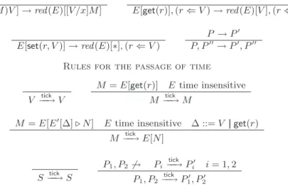
We consider a timed/synchronous extension of our language. Following an established tra-dition, we consider that the computation is divided into instants and that an instant ends when the computation cannot progress. Then we need at least an additional operator that allows to write programs that react to the end of the instant by changing their state in the following instant. We shall see that the termination of the typable programs can be obtained by mapping reductions in the extended language into reductions in the core language. Syntax and Reduction We extend the collection of terms as follows: M ::= · · · || M ⊲ M , where the operator else-next, written M ⊲ N , tries to run M and, if it fails, runs N in the following instant (cf. [7]). We extend the evaluation contexts assuming: E ::= · · · || E ⊲ M , and the elementary evaluation contexts assuming: El ::= · · · || [ ] ⊲ M .
We define a simplification operator red that removes from a context all pending branches else-next: red (E) = [ ] if E = [ ] red (E′) if E = E′⊲ N
El [red (E′)] otherwise, if E = El[E′]
We say that an evaluation context E is time insensitive if red (E) = E. We adapt the reduction rules defined in section 2 as follows:
E[(λx.M )V ] → red (E)[[V /x]M ] E[get(r)], (r ⇐ V ) → red (E)[V ], (r ⇐ V ) E[set(r, V )] → red (E)[∗], (r ⇐ V ) .
specified by the relation−−→ below:tick
V −−→ Vtick S−−→ Stick
M = E[get(r)] E time insensitive M −−→ Mtick M = E[E′[∆] ⊲ N ] ∆ ::= V || get(r) E time insensitive M −−→ E[N ]tick Pi tick −−→ Pi′ i = 1, 2 P1, P2 6→ P1, P2 tick −−→ P′ 1, P2′ .
For instance, we can write (λx.M )get(r) ⊲ N for a thread that tries to read a value from the region r in the first instant and if it fails it resumes the computation with N in the following instant. We can also write ∗ ⊲ N for a thread that (unconditionally) stops its computation for the current instant and resumes it with N in the following instant.
Note that P −−→ only if P 6→. The converse is in general false, but it holds for well-typedtick closed programs (cf. proposition 13). Thus for well-typed closed programs the principle is that time passes (a −−→ transition is possible) exactly when the computation cannot progresstick (a → transition is impossible). Then termination is obviously a very desirable property of timed/synchronous programs.
Typing The typing rules for the terms are extended as follows: R; Γ ⊢ M : (A, e) R; Γ ⊢ N : (A, e′)
R; Γ ⊢ M ⊲ N : (A, e) .
Note that in typing M ⊲ N we only record the effect of the term M , that is we focus on the effects a term may produce in the first instant while neglecting those that may be produced at later instants.
Reduction The decomposition proposition 2 can be lifted to the extended language. There is a third case to be considered besides the two arising in proposition 2 which corresponds to the situation where the redex is under the scope of an else-next. More precisely, in the third case a closed term M is decomposed as E[E′[∆] ⊲ N ] where E is a time insensitive evaluation context and ∆ has the shape V , (λx.N )V , set(r, V ), or get(r).
Focusing on the stratified case, one can adapt the weakening, substitution, and subject reduction properties whose proofs proceed as in proposition 6. The preservation of the type information by the passage of time (tick reduction) can be stated as follows.
If R; ⊢ M, S : (B, e), and M, S −−→ Mtick ′, S′ then S = S′ and there is an effect e′
such that R; ⊢ M′, S : (B, e′).
Notice that the effect of the reduced term might be incomparable with the effect of the term to be reduced. Still the following context substitution property allows to conclude that the resulting term is well-typed.
If R; Γ, x : A ⊢ E[x] : (B, e) where x is not free in the evaluation context E and R; Γ ⊢ N : (A, e′) then R; Γ ⊢ E[N ] : (B, e ∪ e′).
Translation We consider a translation that removes the else-next operator while preserving typing and reduction. Namely, we define a function hi on terms such that hM ⊲ N i = hM i, hxi = x, h∗i = ∗, hri = r, and which commutes with the other operators (abstraction, application, reading, and writing). Also the translation is extended to stores and programs in the obvious way: h(r ⇐ V )i = (r ⇐ hV i), hX1, . . . , Xni = hX1i, . . . , hXni.
Proposition 11 (simulation) (1) If R; Γ ⊢ M : (A, e) then R; Γ ⊢ hM i : (A, e). (2) If R; Γ ⊢ P : (B, e) then R; Γ ⊢ hP i : (B, e).
(3) If R; ⊢ P : (B, e) and P → P′ then hP i → hP′i. (4) A program P terminates if hP i terminates.
The proof of this proposition is direct. In particular, to prove (3) we show that the translation commutes with the substitution and that the translation of an evaluation context is again an evaluation context.
Fixed-point, revisited The typing rule (2) proposed for the fixed-point combinator cannot be applied in the stratified system as the condition r : A −→ B ∈ R and r ∈ e cannot bee satisfied. However, we can still type recursive calls that happen in a later instant.
Proposition 12 (type fixed-point, revisited) The following typing rule for the fixed point
combinator is derived in the stratified system
R; Γ, f : A−−−→ B ⊢ M : (Ae∪{r} −→ B, ∅)e r : A−→ B ∈ Re R; Γ ⊢ fixrf.M : (A
e∪{r}
−−−→ B, ∅)
(3)
We prove this proposition by a direct application of the typing rules and the substitution property (cf. proposition 14). To see a concrete example where the rule can be applied, consider a thread that at each instant writes an integer in a region r′ (we assume a basic type
int of integers):
M = λx.(λz. ∗ ⊲f (x + 1))(set(r′, x))
Then, e.g., (fixrf.M )1 is the infinite behaviour that at the i-th instant writes i in region r′.
One can check the typability of fixrf.M taking as (stratified) region context R = r′ : int, r :
int−−→ 1.{r′}
6
Conclusion
We have introduced a λ-calculus with regions as an abstraction of a variety of concrete higher-order concurrent languages with specific scheduling and interaction mechanisms. We have described a stratified type and effect system and provided a new reducibility candidates interpretation for it which entails that typable programs terminate.
We have highlighted some relevant properties of the interpretation (proposition 7) which could be taken as the basis for an abstract definition of reducibility candidate. The latter is needed to interpret second-order (polymorphic) types (see, e.g., [6]). We believe the proposed proof is both more general because it applies to a variety of interaction mechanisms and
induction on the proof system and because the invariant on the store is easier to manage (the store is not affected by the reduction). This is of course a subjective opinion and the reader who masters [3] may well find our revised treatment superfluous.
We have also lifted our approach to a timed/synchronous framework and derived a form of recursive definition which is useful to define behaviours spanning infinitely many instants. In ongoing work, we have refined the type and effect system to include linear information (in the sense of linear logic) which is relevant both to define deterministic fragments of the calculus and to control better the complexity of the definable programs.
Acknowledgements Thanks to G´erard Boudol for several discussions on [3].
References
[1] R. Amadio and P.-L. Curien. Domains and Lambda Calculi. Cambridge University Press.
[2] R. Amadio and F. Dabrowski. Feasible reactivity in a synchronous π-calculus. In Proc. ACM Principles and Practice of Declarative Programming. pp 221-230, 2007.
[3] G. Boudol. Typing termination in a higher-order concurrent imperative language. In Proc. CONCUR, Springer LNCS 4703:272-286, 2007.
[4] G. Berry and G. Gonthier. The Esterel synchronous programming language. Science of computer pro-gramming, 19(2):87–152, 1992.
[5] Y. Deng and D. Sangiorgi. Ensuring termination by typability. Information and Computation, 204(7):1045-1082, 2006.
[6] J. Gallier. On Girard’s Candidats de Reductibilit´e. In Logic and Computer Science, Odifreddi (ed.), Academic Press, 123-203, 1990.
[7] M. Hennessy, T. Regan. A process algebra of timed systems. Information and Computation, 117(2):221-239, 1995.
[8] J. Lucassen and D. Gifford. Polymorphic effect systems. In Proc. ACM-POPL, 1988. [9] D. Sangiorgi. Termination of processes. Math. Struct. in Comp. Sci., 16:1-39, 2006.
[10] M. Tofte and J.-P. Talpin. Region-based memory management. Information and Computation, 132(2): 109-176, 1997.
[11] N. Yoshida, M. Berger, and K. Honda. Strong normalisation in the π-calculus. Information and Compu-tation, 191(2):145-202, 2004.
A
Proofs
A.1 Proof of proposition 2 (decomposition)
By induction on the structure of M . By the typing hypothesis, M cannot be a variable. If M is a value we are in case 1. Otherwise, M can have exactly one of the following shapes: M1M2, get(M1), set(M1, M2). We consider in some detail the case for application.
The typing rules force M1 and M2 to be typable in an empty context. Moreover M1
must have a functional type. Because of this, if M1 is a value then it must be of the shape
λx.M1′. Moreover, we can apply the inductive hypothesis to M2 and suitably compose with
the evaluation context M1[ ]. If M1 is not a value then we apply the inductive hypothesis to
M1 and suitably compose with the evaluation context [ ]M2. 2
A.2 Proof of proposition 3 (basic properties, unstratified)
Weakening First prove by induction on the proof height that if R, R′ ⊢ and R ⊢ A, (R ⊢
(A, e), R ⊢ A ≤ B) then R, R′ ⊢ A (R, R′ ⊢ (A, e), R, R′ ⊢ A ≤ B). Next, by induction
on the proof height, we show how to transform a proof R; Γ ⊢ M : (A, e) into a proof of
R, R′; Γ, Γ′ ⊢ M : (A, e). 2
Substitution By induction on the proof height of R; Γ, x : A ⊢ M : (B, e).
Subject reduction First we notice that if a term M , of type and effect (A, e), is ready to interact with the store then the region on which the interaction takes place belongs to e. More formally, if R; ⊢ M : (A, e), M ≡ E[∆] and ∆ has the shape get(r) or set(r, V ) then r ∈ e. To prove these facts we proceed by induction on the structure of the evaluation context E. Then we prove the assertion by case analysis on the reduction rule applied relying on the substitution property. 2 A.3 Proof of proposition 5 (type fixed-point)
Suppose r : A −→ B ∈ R and r ∈ e. Then R; ⊢ λx.get(r)x : (Ae −→ B, ∅). By propositione 3(substitution), R; Γ ⊢ M′ : (A−→ B, ∅) where Me ′ = [λx.get(r)x/f ]M . From this we derive: R; Γ ⊢ M′′ : (A−→ B, {r}) where Me ′′ = get(reg
rλx.M′x). This judgement can be weakened
to R; Γ, x : A ⊢ M′′ : (A −→ B, {r}) which combined with R; Γ, x : A ⊢ x : (A, ∅) leads toe R; Γ ⊢ λx.M′′x : (A−→ B, ∅) where λx.Me ′′x = fixrf.M , as required. 2
A.4 Proof of proposition 7 (properties interpretation)
Weakening Suppose R′′ ≥ R′ ≥ R and R′ ⊢ M ∈ R ⊢ (A, e). Then R′; ∅ ⊢ M : (A, e) and by proposition 6(weakening) we know that R′′; ∅ ⊢ M : (A, e). Moreover, an inspection of the definition of R ⊢ (A, e) reveals that if we take a R′′′ ≥ R′′ then the required
properties are automatically satisfied because R′′′≥ R′ and R′⊢ M ∈ R ⊢ (A, e). Extension/Restriction Suppose R′′ ≥ R′ ≥ R and R ⊢ (A, e). We want to show that:
R′′⊢ M ∈ R ⊢ (A, e) iff R′′⊢ M ∈ R′⊢ (A, e) .
Note that R′(R′′) coincides with R(R′′) on dom(R). On the other hand, the proposition 6(subject reduction) guarantees that the reduction of a term of type and effect (A, e) will
We proceed by induction on the structure of the type A.
Suppose A = 1. If R′′ ⊢ M ∈ R ⊢ (A, e) then we know that for any R1 ≥ R′′ we have
that M, R(R1) strongly normalizes to ∗, R(R1). By applying subject reduction, we can
conclude that M, R′(R1) will also strongly normalize to ∗, R′(R1). A similar argument
applies if we start with R′′⊢ M ∈ R′ ⊢ (A, e). Also, this proof schema can be repeated
if A = RegrB.
Suppose now A = A1 e1
−→ A2. If R′′ ⊢ M ∈ R ⊢ (A, e) then we know that for any R1 ≥
R′′, M, R(R1) strongly normalizes to λx.N, R(R1), for some λx.N . Moreover for any
R2≥ R1, we have that R2⊢ V ∈ R ⊢ (A1, ∅) implies R2⊢ (λx.N )V ∈ R ⊢ (A2, e1). By
applying subject reduction, we can conclude that M, R′(R1) will also strongly normalize
to (λx.N ), R′(R1), for some value λx.N . Further, by induction hypothesis on A, if
R2≥ R1 and R2 ⊢ V ∈ R′ ⊢ (A1, ∅) then R2 ⊢ (λx.N )V ∈ R′ ⊢ (A2, e1).
Again, a similar argument applies if we start with R′′⊢ M ∈ R′ ⊢ (A, e).
Subtyping Suppose R ⊢ (A, e) ≤ (A′, e′). We proceed by induction on the proof of R ⊢ A ≤ A′.
Suppose we use the axiom R ⊢ A ≤ A and R′ ⊢ M ∈ R ⊢ (A, e). Then we check that R′ ⊢ M ∈ R ⊢ (A, e′) since R′; ∅ ⊢ M : (A, e′) using the subtyping rule, and the remaining conditions do not depend on e or e′.
Suppose we have A = A1 e1
−→ A2, A′ = A′1 e′
1
−→ A′2, and we derive R ⊢ A ≤ A′ from R ⊢ A′
1 ≤ A1, R ⊢ A2 ≤ A′2, and e1 ⊆ e′1. Moreover, suppose R′ ⊢ M ∈ R ⊢ (A, e).
Then R′; ∅ ⊢ M : (A′, e′), by the subtyping rule. Moreover, if R′′ ≥ R′ and M, R(R′)
reduces to λx.N, R(R′′), we can use the induction hypothesis to show that if R1 ≥ R′′
and R1⊢ V ∈ R ⊢ (A′1, ∅) then R1 ⊢ (λx.N )V ∈ R ⊢ (A′2, e′1).
Strong normalisation This follows immediately from the definition of R ⊢ (A, e).
Reduction closure Suppose R′ ⊢ M ∈ R ⊢ (A, e) and R′′ ≥ R′. We know that M, R(R′′) strongly normalizes to programs of the shape M′′, R(R′′) where M′′ has suitable prop-erties. Then if M, R(R′′) reduces to M′, S′ it must be that S′ = R(R′′) since the
store can only grow. Moreover, by proposition 6(subject reduction), we know that R′′; ∅ ⊢ M′ : (A, e). It remains to check conditions (2) and (3) of the interpreta-tion on R′′ ⊢ M′. Let R′′′ ≥ R′′. We claim M, R(R′′′) reduces to M′, R(R′′′) so
that M′ inherits from M the conditions (2) and (3). To check the claim, recall that M, R(R′′) reduces to M′, R(R′′). Then we analyse the type of reduction performed. The interesting case arises when M reads a value V from the store R(R′′) where, say, R′′ ⊢ V ∈ R1⊢ (B, ∅) and R = R1, r : B, R2. But then we can apply weakening to
conclude that R′′′⊢ V ∈ R1⊢ (B, ∅).
Non-emptiness/Expansion closure We prove the two properties at once, by induction on the proof height of R ⊢ (A, e).
• Suppose R ⊢ (1, e). We take V = ∗. Then for R′ ≥ R we have R′; ∅ ⊢ ∗ : (1, e).
Also, for any R′′ ≥ R′, ∗, R(R′′) converges to itself and satisfies the required properties. Therefore R′⊢ ∗ ∈ R ⊢ (1, e).
This settles non-emptiness. To check expansion closure, suppose R′ ≥ R, R′; ∅ ⊢
M : (1, e), and R′′ ≥ R′. By the decomposition proposition 2, M is either a value
or a term of the shape E[∆] where ∆ is a redex.
If M, R(R′′) does not reduce then M must be the value ∗. Indeed, by the typing
hypothesis it cannot be a region or an abstraction. Also, it cannot be of the shape E[get(r)]. Indeed, suppose R = R1, r : B, R2, then by induction hypothesis on
R1 ⊢ (B, ∅), we know that the store R(R′′) contains at least a value in the region
r .
If M, R(R′′) does reduce then, by hypothesis, for all M′, S′ such that M, R(R′′) → M′, S′ we have that R′′ ⊢ M′ belongs to R ⊢ (A, e) and S′ = R(R′′). This is enough to check the conditions (2) and (3) of the interpretation and conclude that R′ ⊢ M belongs to R ⊢ (A, e).
• The other basic case is R ⊢ (RegrB, e). Then we take as value V = r and we
reason as in the previous case. • Finally, suppose R ⊢ (A1
e1
−→ A2, e). By induction hypothesis on R ⊢ (A2, e1),
we know that there is a value V2 such that for any R′ ≥ R we have R′ ⊢ V2 ∈
R ⊢ (A2, e1). Then we claim that:
R′ ⊢ λx.V2 ∈ R ⊢ (A1 e
1
−→ A2, e) .
First, R′; ⊢ λx.V2 : (A1 e
1
−→ A2, e) is easily derived from the hypothesis that R′; ⊢
V2 : (A2, e1). The second property of the interpretation is trivially fulfilled since
λx.V2 cannot reduce. For the third property, suppose R1 ≥ R′′ ≥ R′ and R1 ⊢
V ∈ R ⊢ (A1, ∅). We have to check that R1 ⊢ (λx.V2)V belongs to R ⊢ (A2, e1).
We observe that R1; ⊢ (λx.V2)V : (A2, e1), and the term (λx.V2)V is neutral.
Moreover, for R2≥ R1, (λx.V2)V, R(R2) → V2, R(R2). Thus we are in the situation
to apply the inductive hypothesis of expansion closure on R ⊢ (A2, e1).
This settles non-emptiness at higher-order. To check expansion closure, suppose R′ ≥ R, R′; ⊢ M : (A1 e
1
−→ A2, e), and M neutral. Then M cannot be a value
and for any R′′ ≥ R′ the program M, R(R′′) must reduce. Indeed, M cannot be
stuck on a read because if r ∈ dom(R) then we know, by inductive hypothesis, that R(R′′)(r) is not-empty. Then we conclude that R′ ⊢ M satisfies properties (2) and (3) of the interpretation because all the terms it reduces to satisfy them. 2
A.5 Proof of theorem 9 (soundness)
We proceed by induction on the proof of R; Γ ⊢ M : (B, e). We shall write [V/x] for [V1/x1, . . . , Vn/xn]. Suppose Γ = x1 : A1, . . . , xn : An, R ⊢ Γ and R′ ≥ R. We let R′ ⊢ V ∈
R ⊢ Γ stand for R′ ⊢ Vi ∈ R ⊢ (Ai, ∅) for i = 1, . . . , n, where V = V1, . . . , Vn.
• Suppose Γ = x1 : A1, . . . , xi : Ai, . . . , xn : An, R; Γ ⊢ xi : (Ai, ∅), R′ ≥ R, and
R′ ⊢ V ∈ R ⊢ Γ. Then [V/x]xi = Vi and, by hypothesis, R′ ⊢ Vi∈ R ⊢ (Ai, ∅).
• Suppose R; Γ ⊢ ∗ : (1, ∅), R′≥ R, and R′⊢ V ∈ R ⊢ Γ. Then [V/x]∗ = ∗ and we know
• Suppose R; Γ ⊢ r : (RegrB, ∅), R′ ≥ R, and R′ ⊢ V ∈ R ⊢ Γ. Then [V/x]r = r and we
know that R′ ⊢ r ∈ R ⊢ (RegrB, ∅).
• Suppose R; Γ ⊢ M : (A′, e′) is derived from R; Γ ⊢ M : (A, e) and R ⊢ (A, e) ≤ (A′, e′).
Moreover, suppose R′ ≥ R, and R′ ⊢ V ∈ R ⊢ Γ. By induction hypothesis, R′ ⊢ [V/x]M ∈ R ⊢ (A, e). By proposition 7(subtyping), we conclude that R′ ⊢ [V/x]M ∈ R ⊢ (A′, e′).
• Suppose R; Γ ⊢ λx.M : (A −→ B, ∅) is derived from R; Γ, x : A ⊢ M : (B, e). Moreover,e suppose R′ ≥ R, and R′ ⊢ V ∈ R ⊢ Γ. We need to check that R′ ⊢ λx.[V/x]M belongs to R ⊢ (A−→ B, ∅). Namely, assuming Re ′′≥ R′ ≥ R and R′′⊢ V ∈ R ⊢ (A, ∅), we have
to show that R′′⊢ [V/x](λx.M )V ∈ R ⊢ (B, e). We observe that R′′; ⊢ [V/x](λx.M )V : (B, e) and that, by weakening R′ to R′′ and induction hypothesis, we know that R′′ ⊢ [V/x, V /x]M ∈ R ⊢ (B, e). Then we conclude by applying proposition 7(expansion closure).
• Suppose R; Γ ⊢ M N : (B, e1∪e2∪e3) is derived from R; Γ ⊢ M : (A e
1
−→ B, e2) and R; Γ ⊢
N : (A, e3). Moreover, suppose R′≥ R, and R′ ⊢ V ∈ R ⊢ Γ. By induction hypothesis,
we know that R′ ⊢ [V/x]M ∈ R ⊢ (A e1
−→ B, e2) and R′ ⊢ [V/x]N ∈ R ⊢ (A, e3). We
have to show that: R′ ⊢ [V/x](M N ) ∈ R ⊢ (B, e1∪ e2∪ e3). Suppose R′′ ≥ R′. Then
[V/x]M, R(R′′) normalizes to λx.M′, R(R′′) for some value λx.M′ and [V/x]N, R(R′′) normalizes to V, R(R′′) for some value V . Further, by reduction closure, we know that R′′ ⊢ λx.M′ ∈ (A e1
−→ B, e2) and R′′ ⊢ V ∈ (A, e3). It is easily checked that the
latter implies R′′ ⊢ V ∈ (A, ∅). By condition (3) of the interpretation, we derive that
R′′⊢ (λx.M′)V ∈ R ⊢ (B, e
1) which suffices to conclude.
• Suppose R; Γ ⊢ set(M, N ) : (1, e1∪ e2∪ {r}) is derived from R; Γ ⊢ M : (RegrA, e1) and
R; Γ ⊢ N : (A, e2). Moreover, suppose R′ ≥ R, and R′ ⊢ V ∈ R ⊢ Γ. By induction
hy-pothesis, we know that R′ ⊢ [V/x]M ∈ R ⊢ (RegrA, e1) and R′ ⊢ [V/x]N ∈ R ⊢ (A, e2).
Then for any R′′≥ R′, [V/x]M, R(R′′) normalizes to r, R(R′′) and [V/x]N, R(R′′)
nor-malizes to V, R(R′′) where R′′ ⊢ V ∈ R ⊢ (A, ∅). Suppose R = R1, r : A, R2. By
definition, R(R′′)(r) = {V′ | R′′⊢ V′ ∈ R1 ⊢ (A, ∅)}. By proposition 7(restriction), we
know that if R′′ ⊢ V ∈ R ⊢ (A, ∅) then R′′⊢ V ∈ R
1 ⊢ (A, ∅). Therefore, V ∈ R(R′′)(r),
and the assignment normalizes to ∗, R(R′′)(r). It follows that R′′ ⊢ [V/x](set(M, N )) belongs to R ⊢ (1, e1∪ e2∪ {r}).
• Suppose R; Γ ⊢ get(M ) : (A, e ∪ {r}) is derived from R; Γ ⊢ M : (RegrA, e).
More-over, suppose R′ ≥ R, and R′ ⊢ V ∈ R ⊢ Γ. By induction hypothesis, we know that R′ ⊢ [V/x]M ∈ R ⊢ (RegrA, e). Then for any R′′ ≥ R′, [V/x]M, R(R′′) normalizes
to r, R(R′′). Thus get([V/x]M ), R(R′′) will reduce to V, R(R′′) where V ∈ R(R′′)(r) which is not empty by proposition 7(not-emptiness). Suppose R = R1, r : A, R2. We
know that R′′ ⊢ V ∈ R1 ⊢ (A, ∅) and by proposition 7(extension) we conclude that
R′′⊢ V ∈ R ⊢ (A, ∅). 2
A.6 Proof of corollary 10 (termination)
(1) By definition, if R ⊢ M ∈ R ⊢ (A, e) then R; ⊢ M : (A, e). On the other hand, as a special case of theorem 9, if R; ⊢ M : (A, e) is derivable then R ⊢ M ∈ R ⊢ (A, e).
(2) Suppose we have R; ⊢ M1, . . . , Mn : e. Then we have R; Mi : (Ai, ei) for i = 1, . . . , n.
By theorem 9, the evaluation of Mi, R(R) is guaranteed to terminate in Vi, R(R), for some
value Vi. Now any reduction starting from M1, . . . , Mn can be simulated step by step by a
reduction of M1, . . . , Mn, R(R) and therefore it must terminate. 2
A.7 Decomposition for the timed/synchronous system Recall that ⊢ef denotes provability in the effect-free system.
Proposition 13 (decomposition extended) If ⊢ef M : A is a well-typed closed thread
then exactly one of the following situations arises where E is a time insensitive evaluation context: (1) M is a value; (2) M = E[∆] and ∆ has the shape (λx.N )V , set(r, V ), or get(r); or (3) M = E[E′[∆] ⊲ N ] and ∆ has the shape V , (λx.N )V , set(r, V ), or get(r).
Proof. By induction on the structure of M . We consider in some detail the case for the else-next (cf. proof A.1 for other cases).
M1 ⊲ M2 We apply the inductive hypothesis to M1, and we have three cases: (1) M1 is a
value, (2) M1 = E1[∆1] with E1 time insensitive, and (3) M1 = E1[E2[∆1] ⊲ N ] with E1
time insensitive. We note that in each case we fall in case 3 where the insensitive evaluation
context is [ ]. 2
A.8 Basic properties for the timed/synchronous extensions
Proposition 14 (basic properties, stratified extended) The following properties hold
in the stratified, timed/synchronous system.
weakening If R; Γ ⊢ M : (A, e) and R, R′⊢ Γ, Γ′ then R, R′; Γ, Γ′⊢ M : (A, e).
substitution If R; Γ, x : A ⊢ M : (B, e) and R; Γ ⊢ N : (A, ∅) then R; Γ ⊢ [N/x]M : (B, e). context substitution If R; Γ, x : A ⊢ E[x] : (B, e) where x is not free in the evaluation
context E and R; Γ ⊢ N : (A, e′) then R; Γ ⊢ E[N ] : (B, e ∪ e′).
subject reduction If R, R′; Γ ⊢ M, S : (B, e), R ⊢ e, and M, S → M′, S′ then R, R′; Γ ⊢ M′, S′ : (B, e), S|dom(R′) = S|dom(R′ ′), and M, S|dom(R) → M′, S|dom(R)′ . Moreover, if
M = M and R, R′⊢ M : (A, e) then M′ = M′ and R, R′; ⊢ M′ : (A, e).
tick reduction If R; ⊢ M, S : (B, e), and M, S −−→ Mtick ′, S′ then S = S′ and there is an effect e′ such that R; ⊢ M′, S : (B, e′).
Proof.
weakening/substitution The proofs of weakening and substitution proceed as in the proof A.2.
context substitution We note that a proof of R; Γ ⊢ M : (A, e) consists of a proof of R; Γ ⊢ M : (A′, e′), where R ⊢ (A′, e′) ≤ (A, e), followed by a sequence of subtyping rules. To prove context substitution, we proceed by induction on the proof R; Γ, x : A ⊢ E[x] : (B, e) and by case analysis on the shape of E.
subject reduction To prove subject reduction, we start by noting that if R; x : A ⊢ E[x] : (B, e) then R; x : A ⊢ red (E)[x] : (B, e). In other terms, the elimination of the pending else-next branches from the evaluation context preserves the typing. Then we proceed by analysing the redexes as in proof A.2.
tick reduction The interesting case is when M = E[E′[∆] ⊲ N ], E is time insensitive, ∆ has the shape V or get(r), and M −−→ E[N ]. Suppose R; ⊢ M : (A, e). Then the typing oftick the else-next guarantees that R; ⊢ E′[∆] : (B, e
1) and R; ⊢ N : (B, e2) for some B, e1, e2
where e1 and e2 may be incomparable. Then we can conclude R; ⊢ E[N ] : (A, e′) where
the effect e′ is contained in dom(R) but may be incomparable with e. 2 A.9 Proof of proposition 11 (simulation)
(1) A straightforward induction on the typing. (2) Immediate extension of step (1).
(3) First we check that the translation commutes with the substitution. Also, we extend the translation to evaluation contexts, assuming h[ ]i = [ ], and check that hEi is again an evaluation context. Then we proceed by case analysis on the reduction rule.
(4) Every reduction in P corresponds to a reduction in hP i. 2 A.10 Proof of proposition 12 (type fixed-point, revisited)
The proof is a variation of the one for proposition 5. Suppose r : A−→ B ∈ R (hence r /e ∈ e). Then R; ⊢ λx.get(r)x : (A −−−→ B, ∅). By proposition 14(substitution), R; Γ ⊢ Me∪{r} ′ : (A −→e
B, ∅) where M′ = [λx.get(r)x/f ]M . From this we derive: R; Γ ⊢ M′′ : (A−→ B, {r}) wheree M′′= get(regrλx.M′x). This judgement can be weakened to R; Γ, x : A ⊢ M′′: (A−→ B, {r})e which combined with R; Γ, x : A ⊢ x : (A, ∅) leads to R; Γ ⊢ λx.M′′x : (A−−−→ B, ∅) wheree∪{r}
λx.M′′x = fixrf.M , as required. 2
B
Summary of syntax, operational semantics, and typing rules
Table 1 summarizes the main syntactic categories, the evaluation rules for the computation within an instant (relation →), and the rules for the passage of time (relation −−→). Tabletick 2 summarizes the typing rules for the unstratified and stratified systems which differ just in the judgements for region contexts and types.
Syntactic categories
x, y, . . . (variables)
r, s, . . . (regions)
e, e′, . . . (finite sets of regions)
A ::= 1 || RegrA || (A e −→ A) || (A−→ B)e (types) α ::= A || B (types or behaviour) R ::= r1: A1, . . . , rn: An (region context) Γ ::= x1: A1, . . . , xn: An (context)
M ::= x || r || ∗ || λx.M || M M || get(M ) || set(M, M ) || M ⊲ M || M, M (terms) V ::= r || ∗ || λx.M (values) v, v′, . . . (sets of value)
S ::= (r ⇐ v) || S, S (stores)
X ::= M || S (stores or terms)
P ::= X || X, P (programs)
E ::= [ ] || EM || V E || get(E) || set(E, M ) || set(r, E) || E ⊲ M (evaluation contexts)
Evaluation rules within an instant
E[(λx.M )V ] → red (E)[[V /x]M ] E[get(r)], (r ⇐ V ) → red (E)[V ], (r ⇐ V )
E[set(r, V )] → red (E)[∗], (r ⇐ V )
P → P′
P, P′′→ P′, P′′
Rules for the passage of time
V −−→ Vtick
M = E[get(r)] E time insensitive M −−→ Mtick
M = E[E′[∆] ⊲ N ] E time insensitive ∆ ::= V || get(r)
M−−→ E[N]tick S−−→ Stick P1, P26→ Pi tick −−→ P′ i i = 1, 2 P1, P2 tick −−→ P′ 1, P2′
Unstratified region contexts and types R ↓ 1 R ↓ B R ↓ A R ↓ α e ⊆ dom(R) R ↓ (A−→ α)e r : A ∈ R R ↓ RegrA ∀ r ∈ dom(R) R ↓ R(r) R ⊢ R ⊢ R ↓ α R ⊢ α R ⊢ α e ⊆ dom(R) R ⊢ (α, e)
Stratified region contexts and types
∅ ⊢ R ⊢ A r /∈ dom(R) R, r : A ⊢ R ⊢ R ⊢ 1 R ⊢ R ⊢ B R ⊢ r : A ∈ R R ⊢ RegrA R ⊢ A R ⊢ α e ⊆ dom(R) R ⊢ (A−→ α)ne R ⊢ α e ⊆ dom(R) R ⊢ (α, e) Subtyping rules R ⊢ α R ⊢ α ≤ α R ⊢ A′≤ A R ⊢ α ≤ α′ e ⊆ e′⊆ dom(R) R ⊢ (A−→ α) ≤ (Ae ′−→ αe′ ′) R ⊢ α ≤ α′ e ⊆ e′⊆ dom(R) R ⊢ (α, e) ≤ (α′, e′)
Terms, stores, and programs R ⊢ Γ x : A ∈ Γ R; Γ ⊢ x : (A, ∅) R ⊢ Γ r : A ∈ R R; Γ ⊢ r : (RegrA, ∅) R ⊢ Γ R; Γ ⊢ ∗ : (1, ∅) R; Γ, x : A ⊢ M : (α, e) R; Γ ⊢ λx.M : (A−→ α, ∅)e R; Γ ⊢ M : (A−→ α, ee2 1) R; Γ ⊢ N : (A, e3) R; Γ ⊢ M N : (α, e1∪ e2∪ e3) R; Γ ⊢ M : (RegrA, e) R; Γ ⊢ get(M ) : (A, e ∪ {r}) R; Γ ⊢ M : (RegrA, e1) R; Γ ⊢ N : (A, e2) R; Γ ⊢ set(M, N ) : (1, e1∪ e2∪ {r}) R; Γ ⊢ M : (A, e) R; Γ ⊢ N : (A, e′) R; Γ ⊢ M ⊲ N : (A, e) R; Γ ⊢ M : (α, e) R ⊢ (α, e) ≤ (α′, e′) R; Γ ⊢ M : (α′, e′) r : A ∈ R ∀ V ∈ v R; Γ ⊢ V : (A, ∅) R; Γ ⊢ (r ⇐ v) : (B, ∅) R; Γ ⊢ Xi: (αi, ei) i = 1, . . . , n ≥ 1 R; Γ ⊢ X1, . . . , Xn: (B, e1∪ · · · ∪ en)