Optimality and non-preemptive real-time scheduling revisited

HAL Id: inria-00074162

https://hal.inria.fr/inria-00074162

HAL is a multi-disciplinary open access

archive for the deposit and dissemination of sci-entific research documents, whether they are pub-lished or not. The documents may come from teaching and research institutions in France or abroad, or from public or private research centers.

L’archive ouverte pluridisciplinaire HAL, est destinée au dépôt et à la diffusion de documents scientifiques de niveau recherche, publiés ou non, émanant des établissements d’enseignement et de recherche français ou étrangers, des laboratoires publics ou privés.

Laurent George, Paul Muhlethaler, Nicolas Rivierre

To cite this version:

Laurent George, Paul Muhlethaler, Nicolas Rivierre. Optimality and non-preemptive real-time scheduling revisited. [Research Report] RR-2516, INRIA. 1995. �inria-00074162�

ISSN 0249-6399

a p p o r t

d e r e c h e r c h e

Optimality and non-preemptive real-time

scheduling revisited

Laurent George,

Paul Muhlethaler,

Nicolas Rivierre

N˚ 2516

Avril 1995

PROGRAMME 1

Architectures parallèles,

bases de données,

réseaux et systèmes distribués

Unité de recherche INRIA Rocquencourt

Domaine de Voluceau - Rocquencourt - B.P. 105 - 78153 LE CHESNAY Cedex (France) Téléphone : +33 (1) 39 63 55 11 - Télécopie : +33 (1) 39 63 53 30

Laurent George, Paul Muhlethaler, Nicolas Rivierre

Laurent.George@inria.fr, Paul.Muhlethaler@inria.fr, Nicolas.Rivierre@inria.fr Programme 1: Architectures parallèles, bases de

données,réseaux et systèmes distribués Projet Reflecs

Rapport de recherche n˚2516- april 1995 27 pages

Abstract: In this paper, we investigate the non-preemptive scheduling problem as it

arises with single processor systems. We extend some previously published results concerning preemptive and non-preemptive scheduling over a single processor. We examine non-idling and idling scheduling issues. The latter are of particular rele-vance in the case of non-preemption..

We first embark on analyzing idling scheduling. The optimality of the non-idling non-preemptive Earliest Deadline First scheduling policy is revisited. Then, we provide feasibility conditions in the presence of aperiodic or periodic traffic. Second, we examine the concept of idling scheduling, whereby a processor can remain idle in the presence of pending tasks. The non-idling non-preemptive Earli-est Deadline First scheduling policy is not optimal since it is possible to find feasi-ble task sets for which this policy fails to produce a valid schedule. An optimal algorithm to find a valid schedule (if any) is presented and its complexity analyzed. This paper shows that preemptive and non-preemptive scheduling are closely related. However, non-preemptive scheduling leads to more complex problems when combined with idling scheduling.

Key-words: real-time, scheduling, non-preemptive, idling, non-idling, optimality,

Résumé : Cet article traite de l’ordonnancement non préemptif sur un

monoproces-seur. Il étend des résultats antérieurs concernant l’ordonnancement préemptif et non préemptif sur un monoprocesseur. Nous examinons les problèmes d’ordonnacement dans les cas non oisifs et oisifs. L’ordonnancement oisif a un intérêt particulier dans le cas non préemptif.

Dans une première partie, l’ordonnancement non oisif est étudié. L’optimalité de la politique d’ordonnancement Echéance la plus Proche en Premier (EDF) non oisive et non préemptive est examinée. Nous dérivons ensuite des conditions de faisabilité en présence de trafic apériodique ou périodique.

La seconde partie est dédiée à l’ordonnancement oisif, pour lequel le processeur peut rester inactif en présence de tâches en attente. La politique d’ordonnancement EDF non oisive et non préemptive n’est pas optimale car il existe des jeux de tâches faisables pour lesquels cette politique ne fournit pas un ordonnancement valide. Un algorithme optimal pour trouver une séquence valide (si elle existe) est présenté et sa complexité est étudiée.

Cet article montre que les problèmes posés par l’ordonnancement préemptif et l’ordonnancement non préemptif sont similaires. Cependant, l’ordonnancement non préemptif conduit à des problèmes plus complexes quand l’ordonnancement oisif est également considéré.

Mots-clé : temps-réel, ordonnancement, non-préemptif, oisif, non-oisif, optimalité,

1. Introduction

This paper addresses the problem of non-preemptive scheduling over a single processor. This problem has received less attention than preemptive scheduling, which has been extensively studied for the past twenty years. In the case of preemptive scheduling, there is a special interest in studying both idling and non-idling scheduling policies. It is recalled that with a non-non-idling scheduling policy, the processor cannot be idle if there are released tasks pending. We will see that there are cases where a valid schedule can be found by an idling scheduling policy whereas no non-idling scheduling policy can find such a valid schedule.

In this paper, most of the results are related to the EDF (Earliest Deadline First) scheduling policy which has been shown to be optimal in many contexts in the case of preemptive scheduling. In fact, we will show that in most cases, results established for preemptive scheduling have a counterpart when considering non-preemptive scheduling.

Section 2 is devoted to introducing the models and the notations used throughout this paper.

Non-idling scheduling issues are addressed in section 3. The first subsection establishes the optimality of the non-idling, non preemptive Earliest Deadline First scheduling policy (NINP_EDF) for any sequence of concrete tasks. The second subsection is concerned with feasibility conditions for the aperiodic/periodic/ sporadic, concrete/non-concrete contexts.

Section 4 is devoted to the analysis of idling scheduling policies. NINP-EDF is shown to be sub-optimal. The problem of finding an optimal scheduling policie in such a context has been shown to be NP-Hard in the strong sense in [GA79]. We propose an exhaustive algorithm (exponential in the worst case) which takes advantage of the partial optimality of NINP-EDF and enables the search to be limited. The behavior of this algorithm is studied with various examples.

2. Notations and definitions

Throughout this paper, we assume the following:

- the EDF scheduling policy uses any fixed tie breaking rule between tasks when they have the same absolute deadline (i.e. release time + relative deadline). - NINP-EDF denotes Non-Idling Non-Preemptive EDF.

- time is discrete (tasks invocations occur and tasks executions begin and termi-nate at clock ticks; the parameters used are expressed as a multiples of clock ticks); see [BHR90] for a justification.

- for the sake of simplicity, we shall use a(i) to describe the tasks and its param-eters. For example, we shall write a(i)=(r_i, e_i, d_i) for a concrete aperiodic task.

We consider the scheduling problem of a set a()={a(1),...,a(n)} of n tasks a(i), over a single processor. By definition:

- A task is said concrete if its release time is known a priori otherwise it is

non-concrete. Then, an infinite number of concrete task sets can be generated from

a non-concrete task set.

- An aperiodic task is invoked once when a periodic (or sporadic) task recurs. Periodic and sporadic tasks differ only in the invocation time. The (k+1)th

in-vocation of a periodic task occurs at time while it occurs at

if the task is sporadic. Notations:

- a concrete aperiodic task a(i), consists of a triple (r_i, e_i, d_i) where r_i is the abso-lute time the task is released, e_i the execution time and d_i the relative deadline. A concrete periodic (or sporadic) task a(i), is defined by (r_i,e_i,d_i,p_i) where p_i is the period of the task.

- a non-concrete aperiodic task a(i) consists of (e_i,d_i). A non-concrete periodic (or sporadic) task a(i) is defined by (e_i,d_i,p_i).

Furthermore, by definition:

- A non-preemptive scheduling policy does not interrupt the execution of any task.

- With idling scheduling policies, when a task has been released, it can either be scheduled or wait a certain time before being scheduled even if the processor is not busy.

- With non-idling scheduling policies, when a task has been released, it cannot wait before being scheduled if the processor is not busy. Notice that an idle pe-riod, i.e. no pending tasks in this case, can have a zero duration.

- A concrete task set a() is said to be synchronous if there is a time when r_i=r_j for all tasks i, ; otherwise, it is said to be asynchronous (the prob-lem of deciding whether an asynchronous task set can be reduced to a synchro-nous one has been shown to be NP-complete in [LM80]).

- A concrete task set a() is said to be valid (schedulable) if it is possible to sched-ule the tasks of a() (including periodic recurrences in the case of periodic or sporadic task sets) so that no task ever misses a deadline when tasks are re-leased at their specified rere-leased times.

- A non-concrete task set a() is said to be valid (schedulable) if every concrete task set that can be generated from a() is schedulable.

- A scheduling policy is said to be optimal if this policy finds a valid schedule when any exists.

3. Non-idling and non-preemptive scheduling

Section 3.1 establishes the optimality of NINP-EDF in the presence of any sequence of concrete tasks. Section 3.2 is concerned with feasibility conditions.

i

∈

[

1 n

,

]

j

∈

[

1 n

,

]

3.1 Optimality of NINP-EDF

Theorem 3a: NINP-EDF is optimal in the presence of any sequence of n concrete

tasks.

Proof: Let s() be a valid schedule; s(1) is the first task scheduled and s(n) is the last

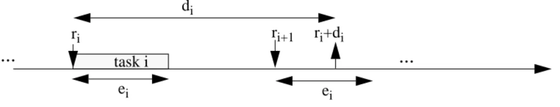
one. Let us introduce a particular reranking of any two successive tasks s(i) and s(i+1) in the schedule. Let t_i (respectively t_i+1) be the beginning of the execution of s(i) (respectively s(i+1)).

s(i) and s(i+1) are left unchanged if r_i+d_i<r_i+1+d_i+1 or r_i+1>t_i. Otherwise, s(i) and s(i+1) are exchanged. The resulting schedule is still valid because r_i+d_i>r_i+1+d_{i +1} (see figure 1).

A full reranking procedure is obtained if we browse through the permutation starting with i=1 to i=n-1. After a finite number of full rerankings, we obtain a stable (i.e. unchanged by a full reranking procedure) valid non-idling, non-preemptive schedule. The finite number comes from the maximum number of times (j for s(j)) that a scheduled task can be reranked which leads to a complexity in O(n2) for the complete procedure.

Let us now show that the obtained schedule is NINP-EDF. Suppose the contrary, then we have a task j such that r_j+d_j<r_j+1+d_j+1 and s(j+1) is released before or at t_j. In such a case the full reranking will not leave the sequence unchanged, which is a contradiction and thus s() is exactly the sequence obtained by NINP-EDF.

EndProof

This theorem means exactly that, in the presence of any sequence of a concrete task set (concrete aperiodic tasks or concrete periodic/sporadic tasks during an interval), NINP-EDF is optimal among non-idling, non preemptive scheduling policies. Such a theorem has already been proved in the following cases:

- preemptive EDF for various traffics [LILA73], [LM80], [MOK83], [CHE87], [BHR90]...

- NINP-EDF with concrete/non-concrete periodic and sporadic task sets [KIM80], [JE91]. Notice that in [JE91], it is shown that the non-preemptive scheduling of concrete periodic tasks is NP-hard in the strong sense. We

be-task 1 task 2 task 3

r₂ r₃ r₃+d₃ r₂+d₂

Valid schedule

r₁+d₁ r₁

task 1 task 3 task 2

r₂ r₃ r₃+d₃ r₂+d₂

Valid NINP_EDF schedule r₁+d₁ r₁

lieve that this problem deals with the establishment of a necessary and suffi-cient condition but not with the optimality of NINP-EDF (in the sense that any valid sequence of schedulable concrete periodic tasks will be scheduled by NINP-EDF).

The optimality of NINP-EDF in the presence of non-concrete aperiodic task set will be addressed in 3.2.1.2.

3.2 Feasibility conditions 3.2.1 Aperiodic tasks

3.2.1.1 Concrete aperiodic tasks

Let a() be a task set of n concrete aperiodic tasks a(i)= (r_i, e_i, d_i). An obvious feasibility condition is to use directly the optimality of NINP-EDF (see section 3.1). This can be done by the following recursive algorithm g(t).

---Initialisation: g(first release)

g(t)

put the new released tasks into the ordered (according to EDF) pending queue IF the first task of the ordered pending queue is a valid (according to EDF)

t <- t + duration of this task IF there are no more task

success /* valid schedule */ ELSE

IF the ordered pending queue is not empty g(t) ELSE g(next release) ENDIF ENDIF ELSE

check /* not valid schedule */ ENDIF

---The complexity of g(t) is O(n) if the tasks are already sorted in increasing order of released time. For a set of randomly ordered tasks, an initial sorting would be required increasing the complexity to O(nlog(n)).

3.2.1.2 Non-concrete aperiodic tasks

Let a() be a task set of n non-concrete aperiodic tasks a(i)= (e_i, d_i). The theorem 3.b is inspired by [JE91] (which establishes the optimality of NINP-EDF and a pseudo-polynomial necessary and sufficient feasibility condition for any non-concrete periodic/sporadic task sets) but adapted to non-non-concrete aperiodic task set.

Theorem 3.b: Let , where , be a set of n non-concrete aperiodic tasks sorted in increasing order by relative deadline (i.e.,

for any pair of tasks and , if i>j, then ). A necessary and sufficient condition for to be schedulable, using NINP-EDF is:

(C1) ; :

Proof: We will demonstrate first that this condition is necessary (part 1) and then

sufficient (part 2). For that purpose, let us define the processor demand in the time

interval [T₁, T₂], written , as the maximum amount of processing time

required by a concrete task set b() (generated from a()) in the interval [T₁, T₂]. will be a function of release, execution time and deadline of the tasks. More

precisely will include:

- all tasks with deadlines in the interval [T₁, T₂] (complete or remaining execu-tion time).

- some tasks with deadlines greater than T₂ (if there are times when in the inter-val [T₁, T₂], where only tasks with deadlines greater than T₂ are pending). b() is schedulable if and only if for all intervals [T₁, T₂], .

Part 1: Condition (C1) is necessary. We will prove the contrapositive, if a() does not satisfy (C1) then there exists a concrete task set b() (generated from a()), that is not schedulable i.e.

; such that .

This leads to the concrete task set b() shown in figure 2, generated from a(), where for some value of i, 1<i≤n, r_i=0 and where the other tasks are released at 1.

We then have: .

Indeed consists of the cost of:

- the execution of task b(i) (since neither preemption nor inserted idle time are allowed, task b(i) must be executed in the interval [0, e_i]).

- plus the processor demand due to the tasks 1 through j in the interval [1, d_j+1] (since (C1) does not hold and since the tasks are sorted in increasing order by deadline, tasks with relative deadlines greater than or equal to d_j do not con-tribute to this processor demand).

As (C1) does not hold then and hence b() is not schedulable.

a(i)

a(j)

d

≥

d

a()

i

∀

,

1

<

i

≤

n

∀

j

,

1

≤

j

<

i

d

j

e

i

–

1

e

k

k

1

∑

+

≥

D

D

D

D

≤

T

–

T

i

∃

,

1

<

i

≤

n

∃

j

,

1

≤

j

<

i

d

e

–

1

e

∑

+

<

d

+

1

e

e

∑

+

<

D

=

D

d

+

1

D

<

The condition is necessary.

Part2: One will show now by contradiction that the condition is also sufficient. Thus, let us suppose that a() satisfies (C1) but is not schedulable. In other words, there exists at least one concrete task set b() (generated from a()) such that b() is not

schedulable, . Let s() be a non valid schedule of b()

such that the deadline of b(j) is not met at time T (T=r_j+d_j). Consider now T₀ the end of the last idle period before T. There are two cases during the busy period [T₀,T]:

- all the scheduled tasks have their absolute deadline less than or equal to T. - the opposite; at least one of the scheduled tasks has its deadline after T. In the first case and since T₀ is the beginning of a busy period, the processor demand during the busy period [T₀,T] is such that:

where if and 0 else.

Indeed, cannot include:

- pending tasks released before T₀ (by definition of T₀ in our non-idling context). - tasks released after (or at) T₀ with relative deadline greater than T-T₀ since we are in the first case (all the scheduled tasks during the busy period [T₀,T] have their absolute deadline less than or equal to T).

At the same time, due to the missed deadline, and therefore one

obtains:

(a) .

Moreover as T=r_j+d_j and as r_j<T₀ is impossible (by definition of T₀ in our non-idling e_i Time 0 1 a(n) a(i) d_i a(1) d₁+1 a(2) d₂+1 a(i-1) d_i-1+1 : : : : e₂ e₁ a(j) d_j+1 : : .... e_j Figure 2

i

∀

,

1

≤ ≤

i

n

b(i)

=

(

r

,

e

, )

d

D

D

δ

e

∑

≤

δ

≥

=

1

T

–

T

≥

d

D

T

–

T

D

<

T

–

T

δ

e

∑

<

context), we just consider . Since we are in the first case (all the scheduled tasks during the busy period [T₀,T] have their absolute deadline before T). If r_j>T₀ leads to missing the deadline of b(j) then it follows that r_j=T₀ leads to missing the deadline of a task b(f) with (by iteration on j, this problem will be detected

later). Then, we examine only r_j=T₀ (i.e. ) and one obtains

.

As a consequence (a) is equivalent to (a’) .

Since (C1) implies that : : (a’) contradicts (C1).

In the second case (see figure 2), let us consider the scheduled task s(i’) as being the last task which is scheduled during the busy period [T₀,T] having a deadline after T (by bijection there exists a(i) such as s(i’) is the execution of a(i)). Notice T_i the start time of the execution of a(i). Similarly to the first case, the processor demand during the busy period [T_i,T] is such that:

.

Indeed, if we use NINP-EDF, cannot include:

- pending tasks at T_i (except a(i)) such as their relative deadline are:

. less than d_i (otherwise, due to NINP-EDF, they should have been executed instead of a(i)).

. greater than or equal to d_i. Since a(i) is the last scheduled task during [T₀,T] with a deadline greater than T.

- tasks released after T_i with relative deadlines greater than T-T_i-1 since we are in the second case and that any scheduled task after T_i has its absolute deadline less than or equal to T.

At the same time, due to the missed deadline, and therefore one

obtains:

(b) .

Moreover as T=r_j+d_j and as r_j<T_i+1 is impossible (otherwise, due to NINP-EDF, a(j)

would have been executed instead of a(i)), we just consider . Since we are

in the second case and that any scheduled task after T_i has its absolute deadline less r j≥T0

f

≥

j

T

–

T

=

d

δ

e

∑

e

∑

=

d

e

∑

<

j

∀

,

1

≤ ≤

j

n

d

e

1

∑

≥

D

D

e

δ

e

∑

+

≤

D

T

–

T

D

<

∑

than or equal to T. If r_j>T_i+1 leads to missing the deadline of b(j) then it follows that r_j=T_i+1 leads to missing the deadline of a task b(f) with (by iteration on j, this

problem will be detected later). Then, we examine only r_j=T_i+1 (i.e.

) and one obtains

.

As a consequence (b) is equivalent to which contravenes to our

initial conditions (C1).

As any non-concrete aperiodic task set a() verifying the necessary conditions is scheduled by NINP-EDF, it follows that:

- the condition is also sufficient.

- NINP-EDF, is optimal in presence of any non-concrete aperiodic task set.

EndProof

Notice that the condition (C1) is in O(n2) and that in [CHE87], a feasibility condition is given for aperiodic preemptive task set which could have been used to establish the above theorem.

3.2.2 Concrete periodic Tasks

The problem of knowing whether in non-idling context, a non-preemptive set of concrete periodic tasks (defined as a(i)=(r_i,e_i,d_i,p_i) for i=1...n) is schedulable has been shown NP-Complete in the strong sense by [JE91]. More precisely, with , a given pseudo-polynomial feasibility condition is shown to be: - necessary and sufficient for any non-concrete periodic/sporadic task set and for

any concrete sporadic task set.

- sufficient but not necessary for any concrete periodic task set since by construc-tion the proof characterizes the worst case which is not necessarily the case for concrete periodic tasks.

In this subsection we show that the feasibility conditions established with preemptive EDF for concrete periodic task sets can be adapted with any non-preemptive, non-idling optimal scheduling policy (e.g. NINP-EDF as shown in theorem 3.a). We illustrate this idea on two well known results:

- First, we extend (section 3.2.2.1) the result of [LM80] to non-preemptive scheduling in order to provide a necessary and sufficient, but exponential, fea-sibility condition. This condition makes it possible to determine if a non-pre-emptive concrete periodic task set is schedulable.

- Then, we study (section 3.2.2.2) the special case of synchronous tasks. In this particular context we adapt the result of [BHR90] in order to obtain a pseudo polynomial necessary and sufficient feasibility condition.

f

≥

j

T

–

T

–

1

=

d

e

δ

e

∑

+

e

e

∑

+

=

d

<

e

–

1

e

∑

+

0

<

e

≤

d

=

p

Let us introduce:

- P = least common multiple of {p₁,...,p_n} the periods of a task set a().

- r = max{r₁,...,r_n} (without loss of generality, we assume that min{r₁,...,r_n} = 0).

3.2.2.1 Asynchronous case

This part is an adaptation of [LM80] to any non-idling, non-preemptive optimal scheduling policy.

Let denote the configuration, at time t, of the schedule s() for

the task set a(). e_i,t is the amount of time for which task T_i has executed from its last release time up until time t (e_i,t =0 if t < r_i).

Notice that if and denote the amount of work done

respectively just before and just after time t, generally we have except if tasks arrive at time t. More precisely, as (only the last release of any task a(i) matters) and if A_t is the set of tasks

arriving at time t, we have: .

Lemma 3.a: Let s() be the schedule of an asynchronous concrete periodic task set

a() (defined as a(i)=(r_i,e_i,d_i,p_i) for i=1...n with ) constructed by any given non-preemptive, non-idling optimal scheduling policy. Then for each instant

t≥r, we have .

Proof: In a non-preemptive context, it is possible to execute a task a(i) even if a

pending task a(j) has a deadline less than a(i). This occurs if a(j) is released during the execution of a(i). Therefore for this Lemma, unlike [LM80], we are obliged to consider, at any time t, the complete configuration of the released task( ) and not tasks one by one.

Due to the first releases times, the pattern of the arriving tasks during is not similar to the pattern of the arriving tasks during . More precisely, the

scheduled tasks during can be deduced from the scheduled tasks

during by removing for every task a(i) each execution during [P, P + r_i] (not arrived in [0, r_i] due to the first release time of a(i)).

As the given scheduling policy is non-idling and as (only the last release of any task a(i) matters), this removing operation can only increase, at time t=r, the sum of the execution time devoted to the execution of the configuration. Then:

.

As the pattern of the releases after is the same as after , it follows that: . EndProof C s()(a() t, ) ei t, i =1 n

∑

=

d

≤

p

-e

∑

–

=

0

<

e

≤ ≤

d

p

≥

+

P

0 r

,

[

]

P P

,

+

r

[

]

0 r

,

[

]

P P

,

+

r

[

]

d

≤

p

r

≥

r

+

P

t

≥

r

t

+

P

t

≥

t

+

P

Lemma 3.a means that as the time elapses there is a tendancy to be late. We are now ready to obtain the result which is again a fairly intuitive result: if an asynchronous concrete periodic task set is feasible then the amount of work executed in similar conditions does not strictly decrease.

Lemma 3.b Let s() be the schedule of an asynchronous concrete periodic task set a()

(defined as a(i)=(r_i,e_i,d_i,p_i) for i=1...n with ) constructed by any given non-preemptive, non-idling optimal scheduling policy. If a() is feasible on one

processor, then there is some instant t in the interval [r+P ,r+2P] when

.

In other words, at t all the released tasks are executed i.e. reaches its maximum.

Proof: First, we show that a processor idle at t cannot be busy during ]t,t+P] and

still has work to do at t+P. For that purpose, let M(T) be the maximum processing time requested by the tasks during [0, T]. By simple algebra, M(T) is given by:

.

The processor is idle at t then the processing time used to execute all the tasks is equal to M(t). Suppose now that the processor is continuously busy (no idle period) in the interval ]t,t+P], then the processing time used to execute all the tasks at t+P is exactly M(t)+P. If at t+P the processor is not idle then we have

(1)

With .

As P is the least common multiple of the periods, M(t+P) can be reformulated as:

then (1) becomes:

leading to

which is not possible on one processor.

0

e

i

≤

d

i

≤

p

i

<

t

e

∑

=

M T

( )

max 0

T

r

i

–

p

i

---,













i

=

1

n

∑

e

i

=

M t

(

+

P

)

>

M t

( )

+

P

∑

∑

∑

∑

We are now ready to complete the proof. Consider t the end of the last idle period before r+2P (i.e. ]t, r+2P] is a busy period). If t<r+P, it comes that

which is impossible on one processor. Thus, if a() is feasible, reaches its maximum during [r+P, r+2P].

EndProof

Theorem 3.c: Let s() be the schedule of an asynchronous concrete periodic task set

a() (defined as a(i)=(r_i,e_i,d_i,p_i) for i=1...n with ) constructed by any given non-preemptive, non-idling optimal scheduling policy. a() is feasible on one processor if and only if (1) all deadlines in the interval [0, r + 2P] are met in the schedule s() and (2) there is some instant t in the interval [r+P,r+2P] when all the pending tasks are executed.

Proof: (the only if part) If a() is feasible on one processor and since we use a

non-idling optimal scheduling policy then s() must be a valid schedule. Thus all deadlines in the interval [0, r+2P] are met in the schedule s() (condition (1)), see [LM80] for a justification of the interval. Furthermore, if a() is feasible, by Lemma 3.b, we have some instant t in the interval [r+P,r+2P] when all released tasks are executed (condition(2)).

(the if part) If conditions (1) and (2) hold it follows that, as the schedule s() is valid in the interval [0, t] and as the pattern of arrival is the same every P after t (i.e. the

configuration reaches its maximum every for each non-negative

integer k), a() is feasible on one processor.

EndProof

Theorem 3.c makes it possible to determine whether a non-preemptive set a() of concrete periodic tasks is schedulable. The complexity of this test is exponential, indeed the problem is known to be NP-Complete in the strong sense (see [BHR90]), but our aim was to show that the feasibility conditions established with preemptive EDF for concrete periodic task sets could be reformulated with any non-preemptive, non-idling optimal scheduling policy.

Let us now show that, as in the case of preemptive scheduling, more refined results can be obtained in the case of synchronous tasks where the total load is known to be under 100%.

3.2.2.2 Synchronous case

The following results are close to [BHR90] since the non-preemptive behavior does not modify the strategy used. More precisely, whatever the context (preemptive or non-preemptive), if the density is less than 1 and if the system is not feasible then there must be a time interval in which too much execution time is required. This

e i p i ----i= 1 n

∑

t

0

<

e

≤ ≤

d

p

t

+

k P

⋅

interval can be combined, whatever the context, with any optimal scheduling policy to establish the proofs.

Let us first show (theorem 3.d) a simple but not optimized w.r.t complexity result in a synchronous non-preemptive context. We will show subsequently (theorem 3.e) that this result, as in [BHR90], can be improved w.r.t complexity.

Theorem 3.d: Let s() be the schedule of a synchronous concrete periodic task set a()

(defined as a(i)=(r_i,e_i,d_i,p_i) for i=1...n with ) and all the release times synchronized at 0) constructed by any given non-preemptive, non-idling optimal scheduling policy. a() is feasible on one processor if and only if all deadlines in the interval [0, P] are met in the schedule s() (condition 1) and at time P, all the pending tasks are executed (condition 2).

Proof: This context is a particular case of theorem 3.c in a synchronous context

where:

- the interval is limited to [0, P] instead of [0, r+2P] (see [LM80]).

- all the release times are synchronous every for each non-negative integer k.

(only if part) If a() is feasible on one processor and since we use a non-idling optimal scheduling policy then s() must be a valid schedule. Thus all deadlines in the interval [0,P] are met in the interval s() (condition (1)). Furthermore, if a() is feasible, by Lemma 3.b, all the released tasks are executed every for each non-negative integer k otherwise at least one deadline is missed (condition (2)).

(if part) If condition (1) and (2) hold it follows that, as schedule s() is valid in the interval [0, P], as the pattern of arrival is the same every P and then as the

configuration reaches its maximum every (for each non-negative

integer k), a() is feasible on one processor.

Endproof

Let denote ( ) the total number of times such that a task a(i)

must be completely scheduled during the interval [t₁, t₂). In [BHR 90] it is shown in the synchronous case with simple algebra that:

.

This result will now allow us to produce a better feasibility condition than Theorem 3.d.

0

<

e

≤ ≤

d

p

k P

⋅

k P

⋅

k P

⋅

η

i

(

t

,

t

)

0

≤

t

<

t

Theorem 3.e: A task system a(), satisfying the context of theorem 3.d and

, with c < 1 is feasible iff:

, with

.

Proof: The proof is based on the fact that t₁ may be chosen to be 0. From the previous algebra, we have:.

As , it follows:

If condition (1) does not hold, and then

.

Hence t₁ may be chosen to be 0 and as , it follows that:

.

Removing the floor function, we have:

which leads to: .

Finally:

,

i.e., if condition (1) does not hold then there exists such

that a deadline is missed.

Endproof.

e

i

p

i

----i

1

n

∑

=

c

η

i

i

=

1

n

∑

t

1

,

t

2









_e

i

≤

t

2

–

t

1

(1)

0

t

t

c

1

–

c

---max p

(

–

d

)

<

<

≤

η

(

0 t

,

–

t

)

max 0

t

–

t

–

d

p

---

+

1

,













=

η

(

0 t

,

–

t

)

max 0

t

–

d

p

---

t

p

----–

+

1

,













≥

η

t

,

t

(

)

=

a

–

b

≥

a

–

b

∑

∑

0

–

t

η

(

0 t

,

)

∑

e

<

˙˙˙

t

–

d

i

---

+













∑

<

t

t

2

–

d

i

+

p

i

p

i

∑

e

i

<

t

2

e

i

p

i

---p

i

–

d

i









_e

i

p

i

---+













∑

=

t

<

ct

+

cmax p

{

i

–

d

i

}

t

c

1

–

c

---max p

{

–

d

}

<

t

c

1

–

c

---max p

{

–

d

}

<

Notice that:

- A consequence, theorem 3.e can be checked in 0(n.max{p_i-d_i}) if , with c < 1.

- Unlike the preemptive case, the worst pattern of arrival in the non-preemptive case is not the synchronous one. Indeed, due to the non-preemptive behavior, a high priority task can be delayed by any task starting its execution just before it (see the pattern examined in theorem 3.b for aperiodic feasibility condition of non-concrete task set).

- In the periodic section, we have shown on two examples that it was easy to de-rive existing feasibility conditions established for preemptive traffics to non-preemptive ones (our aim was not to address every existing improvement [Mok94]).

e

i

p

i

----i

=

1

n

∑

≤

c

4. Idling and non-preemptive scheduling

In this section we schedule a set of n concrete aperiodic tasks a() (a(i)= (r_i, e_i, d_i), (see section 2) sorted in non-decreasing order of released time (r₁=0 by convention).

4.1 Overview

The general problem of finding a feasible schedule in an idling and non-preemptive context is known to be NP-complete [GA79, annex 5]. An exhaustive search leads to examining n! different schedules in the worst case.

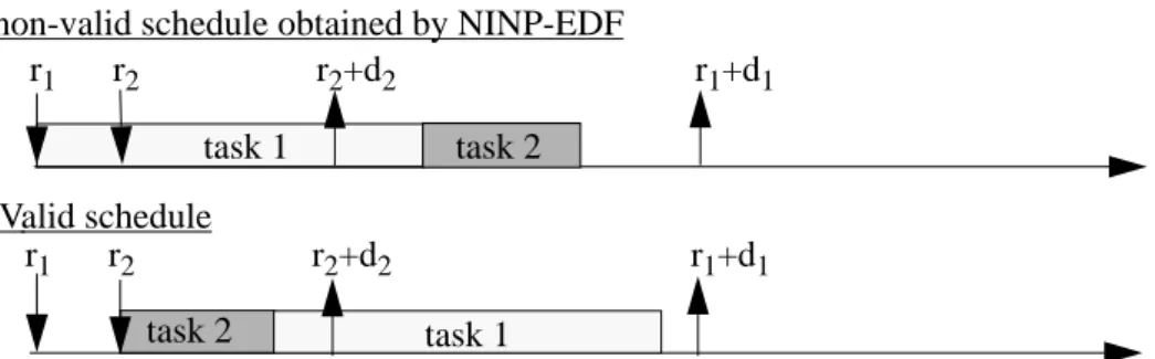
Heuristic techniques can be used [MA84], [MOK83], [ZHAO87] to reduce the complexity. However, this reduction is achieved at the cost of obtaining a potentially sub-optimal solution. For example, NINP-EDF is not optimal for idling scheduling otherwise this would have contradicted the NP-completeness, e.g. the following task set is feasible but NINP-EDF is unable to find a valid schedule (see figure 3).

Optimal decomposition approaches can be used [YUA91], [YUA94], [PC92] to reduce the complexity by dividing the n tasks into m subset. Decomposition, however, is not possible for any task sets.

We now propose a branch and bound scheduling algorithm (see section 4.2) which efficiently limits an exhaustive search. This algorithm always finds a solution when any exists. Although the theoretical complexity is still in n! in the worst case, this algorithm shows good performances at run time (see section 4.3).

4.2 A scheduling algorithm 4.2.1 Description of the algorithm

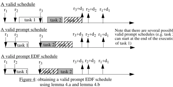
The basic idea is that NINP-EDF is still optimal if it is applied during specific intervals. For this purpose, we will show that any valid schedule can lead to at least one valid prompt schedule (see lemma 4.a) which can itself lead to one valid prompt EDF schedule (see lemma 4.b). Then a branch and bound scheduling algorithm will be presented (see lemma 4.c and theorem 4.a).

Lemma 4.a: If any valid schedule s() of a task set a() exists then it is possible to find

at least one valid schedule s’() for which every task starts either at a released time or at the end of the execution of the last scheduled task. We call s’() a valid prompt

task 1 task 1 task 2 task 2 r₁ r₂ r₂+d₂ r₁+d₁ r₁ r₂ r₂+d₂ r₁+d₁

Figure 3: NINP-EDF is not optimal in idling context non-valid schedule obtained by NINP-EDF

schedule of a() (see figure 4).

Proof: The proof comes from the simple fact that if one can advance the execution

time of the tasks then the schedule is still valid.

To do so consider a task s(i) of s() starting its execution at t1. If s(i) does not start either:

- at t2, the end of the execution of s(i-1), the previous executed task, - or at r_j, one of the possible release times such that t2 < r_j and r_j > r_i, then it is possible to advance the execution of s(i) at t3 such that:

(t3 = t2 or t3 = r_j) and t3 > r_i.

We now call this task s’(i). If we apply this consideration from the first to the last executed task of s(), we are sure that all these tasks will satisfy this lemma. Then we obtain s’() a valid prompt schedule of a().

Note that a valid schedule can lead to several valid prompt schedules, as each task can lead to several possible choices for t3.

EndProof

Lemma 4.b: Let us now suppose that we know a valid prompt schedule (see lemma

4.a), then it is possible to derive another valid prompt schedule satisfying the following property: during any EDF-period, the executed tasks are scheduled according to NINP-EDF. An EDF-period is delimited by two successive release times (notice that, due to the non-preemptive behaviour, if a release time occurs during an execution, the EDF-period is postponed until the end of this execution). We call such a valid prompt schedule a valid prompt EDF schedule (see figure 4).

Proof: Following lemma 4.a, the valid prompt schedule is composed of several

periods. As there are no idling possibilities during an period then each EDF-period can be individually reranked according to the non-preemptive EDF scheduling policy (see theorem 3.a).

EndProof task 1 task 1 task 3 task 2 task 1 r₁ r₂ r3+d3

Figure 4: obtaining a valid prompt EDF schedule r₂+d₂ r₁+d₁ r₃ task 2 task 3 r₁ r_{2 r} 3 task 2 r₁ r_{2 r3} task 3

A valid schedule

A valid prompt schedule

A valid prompt EDF schedule

using lemma 4.a and lemma 4.b r₃+d₃ r₂+d₂ r₁+d₁

r₃+d₃ r₂+d₂ r₁+d₁

Note that there are several possible valid prompt schedules (e.g. task 2 can start at the end of the execution of task 1)

Lemma 4.c: If a valid schedule exists then we can derive at least one valid prompt

EDF schedule.

Proof: It is straightforward from lemma 4.a and lemma 4.b (see figure 4). EndProof

We are now ready to give a necessary and sufficient conditionv concerning the feasibility of a contrete task set in Idling non-preemptive context.

Theorem 4.a: The following recursive algorithm f(t) finds out whether a valid

schedule exists.

---Initialization : f(first release)

f(t)

A: put the new released tasks into the ordered (according to EDF) pending queue IF there is at least one new pending task

set the current pending task as the first of the ordered (according to EDF) pending queue ENDIF

B: IF the current pending task is valid (according to EDF) t <- t + duration of this task /* case a */ IF there are no more task

success /* valid schedule */ ELSE

IF the ordered pending queue is not empty f(t) ELSE f(next release) ENDIF ENDIF ELSE

check /* not valid schedule */ ENDIF

/* this part is implied by the idling mode */

reset the ordered pending queue and the current pending task as it was before B:

IF the current pending task is valid (according to EDF) /* otherwise no idling can be successful */ IF the ordered pending queue is not empty /* otherwise go to the next release */

set the current pending task as the next task of the ordered pending queue /* case b) f(t)

ELSE

f(next release) /* case c */ ENDIF

ENDIF

reset the ordered pending queue and the current pending task as it was before A:

---Proof: By its very nature, the previous algorithm searches all the valid prompt EDF

schedules (i.e. all the valid schedules satisfying lemma 4.c). Indeed if a valid schedule exists then at least one valid prompt EDF schedule satisfying lemma 4.c also exists and therefore the previous algorithm finds it.

4.2.2 Comments and example

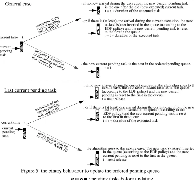
This recursive algorithm f(t) is an extension, in idling context, of the algorithm g(t) presented in section 3.2.1.1 (the updated parts are in bold). In order to search all the idling possibilities satisfying lemma 4.c the algorithm maintains (see figure 5),

at each call, an ordered queue (according to EDF) of the pending tasks and a pointer of the current pending task (which will be the next possible task executed in the current EDF-period). Then the ordered pending queue is updated by one of the three following cases: temporary forgetting

General case

. if no new arrival during the execution, the new current pending task

of the current pending task (

case b

) . the new current pending task is the next in the ordered pending queue.

execution of the current pending task (case a ) current pending task current time = t

idling period until the next release (

case c

) . the algorithm goes to the next release. The new task(s) is(are) inserted

Last current pending task

. or if there is (at least) one arrival during the current execution, the new

. if no new arrival during the current execution, the algorithm goes to the next release. the new task(s) is(are) inserted in the queue

is the one after the old (now executed) current task. t = t + duration of the executed task

task(s) is(are) inserted in the queue (according to the to the first in the queue

t = t

t = t + duration of the executed task

EDF policy) and the new current pending task is reset

(according to the EDF policy) and the new current pending is reset to the first in the queue.

t = next release

. or if there is (at least) one arrival during the current execution, the new task(s) is(are) inserted in the queue (according to the to the first in the queue

t = t + duration of the executed task

EDF policy) and the new current pending task is reset

in the queue (according to the EDF policy) and the new current pending is reset to the first in the queue. t = next release

: pending tasks before updating

: next released task

- the current pending task is executed (case a). The ordered pending queue is then updated by removing the executed task and by taking account of possible new release tasks during the execution

- the current pending task is temporarily forgotten (until the next EDF-period). There are two possibilities:

. the new current pending task is the next one in the ordered pending queue (case b).

. there are no more tasks in the ordered pending queue. This leads to an idling period until the next EDF-period (case c).

Of course, in order to allow the search of all the possible valid prompt EDF, at each new release time (which leads to a new EDF-period) the current pending task is reset to the first task of the ordered pending queue.

Therefore the whole algorithm produces a binary tree where every leaf may provide (if there is no deadline failure) a valid prompt EDF schedule:

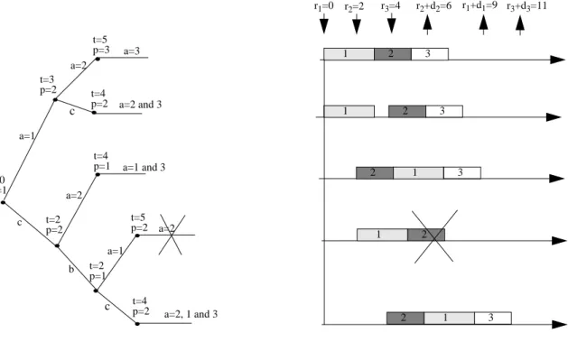
Let us give now a short example (see figure 6) for three tasks. At run time, we find: - four valid prompt EDF schedules

- and one non-valid schedule

t=0 p=1 t=3 p=2 t=5 p=3 t=4 p=2 r₁=0 r2=2 r₃=4 r2+d2=6 r1+d1=9 r3+d3=11 t=2 p=2 t=4 p=1 t=2 p=1 t=5 p=2 t=4 p=2 1 2 3 1 2 3 1 2 3 1 2 1 2 3 a=1 a=2 a=3 a=2 and 3 a=2 a=1 and 3 a=2 a=2, 1 and 3

Figure 6: execution of 3 tasks (a()= {a(1)=(0,3,9), a(2)=(2,2,4), a(3)=(4,2,7)}). - above each node,t is the current time and p is the current pending task.

a=1 c

b

- between two nodes, the case considered (a,b,c see figure 5). The case a is followed by

c c

4.3 Performances

Although the potential number of solutions for the previous algorithm f(t) (see section 4.3.1) is n!, we will see in 4.3.2 that this number is generally much less.

4.3.1 Complexity

In order to compute the complexity of this tree algorithm, we will establish the theoretical number of solutions generated by n tasks. Intuitively this number is maximized when the idling behavior is not limited (fully developed tree) i.e. when it is always possible to compute the pending tasks between two release-times.

More formally let be a node(s,d+1) generated from a node(f,d) where:

- d+1 is the current depth (i.e. the release time of the node(s,d+1)). - f is the number of pending tasks at depth d (the previous release time).

- s is the number of pending tasks ( ) at depth d+1 (the current

re-lease time).

It follows that:

- a node(f,d) can generate f+1 nodes(s,d+1) where f-s+1 is the number of execut-ed tasks from depth d to depth d+1 (i.e. from the previous release time to the current release time).

- a node(s,d+1) is weighted by the number of non-ordered sequences

of f-s+1 executed tasks among the f pending task. Indeed, due to the EDF pol-icy during an EDF-period (see lemma 4.b, section 4.2), only one order is avail-able for each sequence of executed tasks.

Let us see an example of the exhaustive graph (see figure 7) built with 3 tasks. Note that, as we search the number of possible leaves and not the way to obtain them (case a, b and c of the algorithm), we directly use the node(f,d) formalism which is more concise (then every node is weighted by the number of possible ordered

sequences i.e. by ).

For 3 tasks, there are 3! = 6 potential valid prompt EDF schedules that may be compared with the real example (see figure 6) which leads only to four valid prompt

s,d+1

C_ff-s+1

1

≤ ≤

s

f

+

1

C

schedules and one non-valid schedule (see the discussion in section 4.3.2).

More generally, we shall now prove that the number of leaves generated by an original node(1,1) on depth n is n!. For that let us first consider the following theorem proved by induction

theorem 4.b: The number of leaves generated by a node(f,d) at depth is: P(f,r) = r!(r)f-1 (with r=d’-d+1).

proof: Clearly, the original node(1,1) generates at depth 1: P(1,1) = 1 (i.e. 1!(1)1-1) leaf.

Assume now that the theorem is valid at depth d’, then P(f,r) = r!(r)f-1. As a node(f,d) generates at depth d+1, f+1 nodes(s,d+1) weighted by:

with . As each node(s,d+1) can generate, P(s, r) = r!(r)s-1 leaves. Then a node(f,d) can generate at depth d’+1 (relative depth r+1):

And then from binomial theorem,

.

It follows that the assumption is still valid at the relative depth r+1.

End Proof 2,2 1,1 1,2 3.3 2,3 1,3

C

C

C

C

C

d=1

d=2

d=3

C

C

The number of leaves is

C

+ C

+C

+ C

+ C

=3!

C

Figure 7: complexity in the presence of 3 tasks

d

′

≥

d

f

∀

∈

N

C

1

≤ ≤

s

f

+

1

P f r

(

,

+

1

)

C

r! r

( )

∑

r!

C

( )

r

∑

r!

C

( )

r

∑

=

=

=

As a result the number of leaves generated by a node(1,1) at depth n is

P(1,n) = n!(n)

= n!.

4.3.2 Discussion

Of course a theoretical number of solutions in n! is not satisfactory yet the algorithm f(t) can be considered for the following reasons:

- due to the lemmas 4.a and 4.b (see section 4.2) the search is not exhaustive. More precisely the idling behavior is strongly limited (only the potential valid prompt EDF schedules are considered) without the risk of missing a solution. - at run-time a tree search is limited by the tasks parameters leading to:

. deadline failures which stop the current tree search path. It follows (see 4.3.1) that if the search stops on a node(f,d), P(f,r)=(r)!(r)f-1 potential sched-ules are not explored (with r=n-d+1).

. gathering release time disables idling development. Indeed, suppose a node(f,d). This node will generate from theorem 4.b P(f,r)=(r)!(r)f-1 leaves (with r=n-d+1). Suppose now that the node(f,d) at the next release time sees not only one task but k tasks. Then it comes that the number of leaves gen-erated by the node(f,d) is:

Which is inferior to (r)!(r)f-1for k>1 (and equal for k=1). Indeed, for k>1

Then the gathering of release time limits the tree search path.

In order to evaluate the performances of the algorithm f(t) at run time (for any concrete aperiodic task set a()={a(1),...,a(n)} where each task a(i)= (r_i, e_i, d_i) is as defined in section 2 and where the tasks are sorted in non-decreasing order by release time) let us define the following parameters:

- s_a() which is the number of valid prompt schedules of a() found at run time. - c_a() which is the cost i.e. the number of valid and non-valid EDF prompt

sched-ules of a() found at run time (remember that a non-valid EDF prompt schedule is necessarily incomplete due to the deadline failure).

- the cost ratio cr_a() = c_a()/n!. - the efficiency ratio er_a() = s_a()/c_a().

Let’s start the performance analysis by describing two sufficient conditions leading to good performances:

- If , and then a() leads to

C f s P f( +k–1–s,r–k) s=0 f

∑

∑

(

r

–

k

+

1

)

i

∀

,

1

≤ ≤

i

n

–

1

r

i

+

e

i

≥

r

i

+

d

i

r

i

≥

r

i

+

e

i

only one valid schedule.

Indeed this situation means that any idling search lead to invalid schedules, only the pure prompt and non-idling EDF policy leads to a valid schedule (see figure 8). Therefore the tree is reduced to a unique path from the root to an unique leaf (we call this situation an efficient limited tree). This unique path is exactly the one studied in section 3.2.1.1.

- If , then every potential prompt EDF

schedule is valid.

Indeed this situation means that, due to the late deadline, all the tree search paths lead to valid schedules. Therefore the tree is fully developed (we call this situation an efficient large tree)..

The efficient limited tree situation leads to one solution with a very limited search (s_a()=1, c_a()=n and then cr_a()=n/n!, er_a()=1/n) when the efficient large tree leads to a search of exponential complexity but also to many valid schedules (s_a()=n!, c_a()=n! and then cr_a()=1, er_a()=1).

Of course these two sufficient conditions seem strongly restrictive however it is possible to describe a lot of efficient scenarios like those.

The real conjecture is to know if there exist situations leading to an inefficient large tree i.e. search of exponential complexity leading to few valid schedules (in worst case s_a() = 0, c_a() = n! and then cr_a() = 1, er_cost = 0). In order to examine this possibility, let us now give some simulations (see table 1) to estimate this efficiency in a real context. We make use of random task sets and give, for each task number, an average on ten runs. These results show that:

- the limitation of the tree search at run time (due to deadline failures, regrouping of release time...) is strongly marked when the number of task increases (the cost ratio cr_a() decreases). This limits the computation time.

- the efficiency ratio er_a() is non-negligible (around 0.5) and is not impacted by the task number.

This lead (when if it is sufficient to obtain only one valid schedule for a given task set) to propose the following heuristic: search at random some path in the tree until finding one valid schedule. Technical results concerning the efficiency of the

i

∀

,

1

≤ ≤

i

n

d

r

e

∑

+

=

Figure 8: efficient limited tree r_i+1

d_i

e_i e_i

algorithm f(t) will be developed in further papers.

5. Conclusion

EDF is extensively studied in this paper for non-preemptive scheduling.

In the case of non-idling scheduling, EDF is shown to be optimal. Feasibility conditions are established for many patterns of arrival laws (aperiodic/periodic, concrete/non-concrete, synchronous/asynchronous...). This paper shows that preemptive and non-preemptive scheduling are closely related.

The case of idling scheduling opens the door to more complex problems. Indeed, any valid non-idling schedule is also valid in idling scheduling but the reverse is not true. Although the theoretical number of valid schedule is n!, we have shown that non-idling EDF could be applied during specific intervals, called EDF-periods. This property allows to propose an algorithm which efficiently finds valid schedules.

6. references

[BHR90] K.Sanjoy, L.E.Rosier, R.R.Howell, “Algorithms and Complexity Concerning the Preemptive Scheduling of Periodic, Real-Time Tasks on One Processor”, Real Time Systems 90 p 301-324.

[CHE87] H.Chetto, M.Chetto, "How to insure feasibility in a distributed system for real-time control?", Int. Symp. on High Performance Computer Systems, Paris, Dec. 1987.

[GA79] M. R. Garey, D. S. Johnson, “Computer and Intractability, a Guide to the Theory of NP-Completeness”, W. H. Freeman Company, San Francisco, 1979.

Table 1: Simulation results

Task number n! success s_a() cost c_a() cost ratio cr_a() efficiency ratio er_a() 3 6 2 4 0.67.. 0.5 6 720 88 174 0.24.. 0.51.. 8 40320 1892 3668 0.09.. 0.52.. 10 3.63.. 106 10658 30046 0.008.. 0.35.. 12 479.. 106 670240 2421600 0.005.. 0.28..

[JE91] K. Jeffay, D. F. Stanat, C. U. Martel, “On Non-Preemptive Scheduling of Periodic and Sporadic Tasks”, IEEE Real-Time Systems Symposium, San-Antonio, December 4-6, 1991, pp 129-139.

[KIM80] Kim, Naghibdadeh, Proc. of Perf. 1980, Assoc. Comp. Mach. pp 267-276, “Prevention of task overruns in real-time non-preemptive multiprogramming systems”

[LILA73] C.L Lui, James W. Layland, “Scheduling Algorithms for multiprogramming in a Hard Real Time Environment”, Journal of the Association for Computing Machinery, Vol. 20, No 1, Janv 1973.

[MA84] P. R. Ma, "A model to solve Timing-Critical Application Problems in Distributed Computing Systems”, IEEE Computer, Vol. 17, pp. 62-68, Jan. 1984.

[MOK83] A.K. Mok, “Fundamental Design Problems for the Hard Real-Time Environments”, May 1983, MIT Ph.D. Dissertation.

[LM80] J. Y.T.Leung et M.L.Merril, “A note on preemptive scheduling of periodic, Real Time Tasks”, Information processing Letters, Vol. 11, num. 3, Nov 1980.

[MC92] P. Muhlethaler, K. Chen, “Generalized Scheduling on a Single Machine in Real-Time Systems based on Time Value Functions”, 11th IFAC Workshop on Distributed, Computer Control Systems (DCCS’92), Beijing, August 1992

[YUA91] Xiaoping Yuan, “A decomposition approach to Non-Preemptive Scheduling on a single ressource", Ph.D. thesis, University of Maryland, College Park, MD 20742.

[YUA94] Xiaoping Yuan, Manas C. Saksena, Ashok K. Agrawala, “A decomposition approach to Non-Preemptive Real-Time Scheduling”, Real-Time Systems, 6, 7-35 (1994).

[ZHAO87] W. Zhao, K. Ramamritham, J. A. Stankovic. “Scheduling Task with Resource requirements in a Hard Real-Time System”, IEEE Trans. on Soft. Eng., Vol. SE-13, No. 5, pp. 564-577, May 1987.

Éditeur

Inria, Domaine de Voluceau, Rocquencourt, BP 105 LE CHESNAY Cedex (France)

ISSN 0249-6399