Design-Space Exploration of Stream Programs through Semantic-Preserving Transformations

HAL Id: hal-00447376

https://hal.archives-ouvertes.fr/hal-00447376

Preprint submitted on 14 Jan 2010

HAL is a multi-disciplinary open access

archive for the deposit and dissemination of

sci-entific research documents, whether they are

pub-lished or not. The documents may come from

teaching and research institutions in France or

abroad, or from public or private research centers.

L’archive ouverte pluridisciplinaire HAL, est

destinée au dépôt et à la diffusion de documents

scientifiques de niveau recherche, publiés ou non,

émanant des établissements d’enseignement et de

recherche français ou étrangers, des laboratoires

publics ou privés.

Design-Space Exploration of Stream Programs through

Semantic-Preserving Transformations

Pablo de Oliveira Castro, Stéphane Louise, Denis Barthou

To cite this version:

Pablo de Oliveira Castro, Stéphane Louise, Denis Barthou. Design-Space Exploration of Stream

Programs through Semantic-Preserving Transformations. 2009. �hal-00447376�

Design-Space Exploration of Stream

Programs through Semantic-Preserving

Transformations

Pablo de Oliveira Castro

_{, St ´ephane Louise}

_{and Denis Barthou}

1_{CEA, LIST, Embedded Real Time Systems Laboratory,} 2_{University of Bordeaux - Labri / INRIA} F-91191 Gif-sur-Yvette, France; 351, cours de la Lib ´eration, Talence, F-33405 France; {pablo.de-oliveira-castro, stephane.louise}@cea.fr [email protected]

✦

Abstract

Stream languages explicitly describe fork-join parallelism and pipelines, offering a powerful programming model for many-core Multi-Processor Systems on Chip (MPSoC). In an embedded resource-constrained system, adapting stream programs to fit memory requirements is particularly important.

In this paper we present a design-space exploration technique to reduce the minimal memory required when running stream programs on MPSoC; this allows to target memory constrained systems and in some cases obtain better performance. Using a set of semantically preserving transformations, we explore a large number of equivalent program variants; we select the variant that minimizes a buffer evaluation metric. To cope efficiently with large program instances we propose and evaluate an heuristic for this method.

We demonstrate the interest of our method on a panel of ten significant benchmarks. As an illustration, we measure the minimal memory required using a multi-core modulo scheduling. Our approach lowers considerably the minimal memory required for seven of the ten benchmarks.

1

I

The recent low-consumption Multi-Processors Systems on Chip (MPSoC) enable new computation-intensive embedded applications. Yet the development of these applications is impeded by the difficulty of efficiently programming parallel applications. To alleviate this difficulty, two issues have to be tackled: how to express concurrency and parallelism adapted to the architecture and how to adapt parallelism to constraints such as buffer sizes and throughput requirements.

Stream programming languages [1][2][3] are particularly adapted to describe parallel programs. Fork-join parallelism and pipelines are explicitly described by the stream graph, and the underlying data-flow formalism enables powerful optimization strategies.

As an example, the StreamIt [1] framework defines transformations of dataflow programs en-hancing parallelism through fission/fusion operations. These transformations are guided by greedy heuristics. However, to our knowledge, there is no method for the systematic exploration of the design space based on the different expressions of parallelism and communication patterns. The main difficulty comes from the definition of a space of semantically equivalent parallel programs and the complexity of such exploration.

In this paper we propose a design space exploration technique that generates, from an initial program, a set of semantically equivalent parallel programs, but with different buffer, communication and throughput costs. Using an appropriate metric, we are able to select, among all the variants, the one that best fits our requirements. We believe that our approach is applicable to buffer, communi-cation and throughput requirements, yet in this paper we only consider memory requirements. Study of the other requirements will be the object of future works.

The buffer requirements of stream programs depend not only on the different rates of its actors but also on the chosen mapping and scheduling. We demonstrate the memory reduction achieved by our technique using the modulo scheduling execution model. Kudlur and Mahlke[4] use modulo scheduling to minimize the throughput when mapping stream programs on a multi-core processor. Choi et al[5] extend this method to cope with memory and latency constraints. They introduce the

Memory-constrained Processor Assignment for minimizing Initialization Interval(MPA-ii) problem which

S J

c2 p2

c1 p1

Fig. 1. The split node S alternatively outputs p1 then p2 elements on the two edges, while the join node J takes alternatively c1 and c2 elements from its incoming edges.

MPA-ii achieves memory reductions as high as 80%. Yet our exploration method could also be applied

to other scheduling and mapping techniques, it is not particularly tied to MPA-ii. The contributions of this paper are:

• a theoretical framework to check if a stream program transformation is valid; • a general set of valid stream transformations;

• a terminating exhaustive search algorithm for the implementation space generated by the above

transformation set;

• an heuristic based on graph partitioning to explore very large program instances;

• a design space exploration that minimizes memory requirements on a large set of programs.

Section 2 presents the data-flow formalism used. The transformations modifying the granularity of the elements of our program and producing semantically equivalent variants are described in Section 3. Section 4 presents the exploration algorithm built upon these transformations and the algorithm termination proof. Section 5 reviews the MPA-ii problem[5] that we use to illustrate the benefits of our exploration method and section 6 presents a buffer size metric evaluation. In Section 7 we present our experimental methodology and our results. Finally, Section 8 presents related works.

2

F

In our approach a program is described using a cyclo-static data flow (CSDF) graph where edges represent communications and nodes are either data reorganization operations or computation filters. Nodes represent the CSDF actors, the node label indicates the node kind (sometimes followed by a number to allow easy referencing); edges denote inputs and outputs. When necessary, the node productions or consumptions are indicated on their associated edges. As an example consider figure 1: a split node with productions (p1, p2) is connected to a join node with consumptions (c1, c2).

Our stream formalism is very close to Streamit [1]; we consider the following set of nodes:

2.1 Input and Output nodes

Source I(l): a source models a program input. It has an associated size l. The source node is fired only once and writes l elements to its single output. If all the elements in the source are the same, the source is constant and denoted by the node C(l).

Sink O: a sink models a program output. It consumes all elements on its single input. If we never observe the consumed elements, we say the sink is trash and we write the node T.

2.2 Splitter and Joiner nodes

Splitter and joiners correspond to the expression of data parallelism and communication patterns.

Join round-robin J(c1. . . cn) : a join round-robin has n inputs and one output. We associate to each

input i a consumption rate ci ∈ N⋆. The node fires periodically. In its kth firing the node takes cu,

where u = (k mod n) + 1, elements on its uth _{input and writes them on its output. As in a classic}

CSDF model, nodes only fire when there are enough elements on their input. When the node has consumed elements on all its inputs, it has completed a cycle and starts all over again.

Split round-robin S(p1. . . pm) : a split round-robin has m outputs and one input. We associate to

each output j a production rate pj∈ N⋆. In its kthfiring the node takes pv, where v = (k mod m)+1,

elements on its input, and writes them to the vth_output.

Duplicate D(m)has one input and m outputs. Each time this node is fired, it takes one element on the input and writes it to every output, duplicating its input m times.

2.3 Filters

A filter node F(c1. . . cn, p1. . . pm) has n inputs and m outputs. To each input i is associated a

consumption rate ci, and to each output j a production rate pj. The node is associated to a pure

function f computing from n inputs m outputs. The node fires when for each input i there is at least ci available elements.

Fig. 2. An abstract CSDF transformation.

2.4 Schedulability

We can schedule a CSDF graph in bounded memory if it has no deadlocks (it is live) and if it admits a steady state schedule (it is consistent) [6][7].

A graph is live when no deadlocks can occur. A graph deadlocks if the number of elements received by any sink remains bounded no matter how much we increase the size of the sources.

A graph is consistent if it admits a steady state schedule, that is to say a schedule during which the amount of buffered elements between any two nodes remains bounded. A consistent CSDF graph G with NG nodes admits a positive repetition vector ~qG = [q1, q2, . . . , qNG] where qi represents the

number of cycles executed by node i in its steady state schedule. Given two nodes u, v connected by edge e. We note β(e) the elements exchanged on edge e during a steady state schedule execution. If node u produces prod(e) elements per cycle on edge e and node v consumes cons(e) elements per cycle on edge e,

β(e) = prod(e) × qu= cons(e) × qv (1)

3

S

S

In this section we present the transformations that are used to generate semantically preserving variants of the input program. In sec. 3.1 we define what is a semantically preserving (or admissible) transformation. In sec.3.2 we present a set of useful and admissible transformations.

The graph transformation framework presented here follows the formulation given in [8]. A transformation T (fig. 2) applied on a graph G and generating a graph G′ _{is denoted G −→ G}T ′_.

It is defined by a matching subgraph L ⊆ G, a replacement graph R ⊆ G′ _{and a glue relation g that}

binds the frontier edges of L (edges between nodes in L and nodes in G\L) to the frontier edges of R.

The graph transformation works by deleting the match subgraph L from G thus obtaining G\L. After this deletion, all the edges between G\L and L are left dangling. We then use the glue relation to paste R into G\L obtaining G′_.

A sequence of transformations applied to a graph define a derivation:

Definition 1: A derivation of a graph G0 is a chain of transformations that can be applied

succes-sively to G0: G0 T0 −→ G1. . . Tn −−→ . . .. 3.1 Admissible transformations

In this section we define formally the properties that a transformation must possess to preserve the semantic of a program. In lemma 1, we also give a sufficient condition for a transformation to be semantically preserving. We suppose without loss of generality that our stream graphs are connex.

The ordered stream of tokens for a given edge e defines the trace of the edge, denoted t(e). We consider a prefix order ≤ on traces: x ≤ y ⇒ (x infinite ∧ x = y) ∨ (x = y[0 .. x − 1]). We also extend ≤ for tuples: u ≤ v ⇒ ∀k, u[k] ≤ v[k].

Sink and Source nodes have a single edge, thus with no ambiguity, we will consider that the trace of a Source or Sink node is the trace of its unique edge. The input traces and output traces are defined respectively as I(G) = [t(i) : i ∈ Sources] and O(G) = [t(o) : o ∈ Sinks]. Furthermore, for a subgraph H ⊆ G we define I(H) as the traces on the input edges of H and O(H) as the traces on the output edges of H. The tuple of the lengths of each sink trace is noted O(G) = [t(o) : o ∈ Sinks].

Definition 2: Given a CSDF graph G, a transformation G−T→ G′ _{is admissible iff}

I(G) = I(G′) ⇒ O(G) ≤ O(G′) (2)

G is consistent ⇒ G′ _{is consistent (3)}

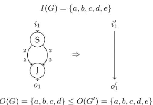
I(G) = {a, b, c, d, e}

O(G) = {a, b, c, d} ≤ O(G′_{) = {a, b, c, d, e}} i1 o1 S J 2 2 2 2 ⇒ i′ 1 o′ 1

Fig. 3. Example of a transformation that is only possible under the weak condition of eq.2

In other words, T preserves the semantics of G if T preserves consistency, liveness and if for the same inputs, the graph generated by T , G′_{, produces at least the same outputs as G. We show in}

lemma 1 proof, that (2) ⇒ (4).

This weak definition of semantics preservation defines a large class of admissible transformations. If we had enforced a strict preservation of the output (O(G) = O(G′_{)), some of the transformations}

presented in section 3.2 would not be possible. Indeed these transformations relax the communication rates to achieve simplifications. Take for example the transformation in figure 3, the split and join nodes seem useless since they do not change the order of the elements, yet they impose that elements are always consumed in pairs. If we simplify this pattern, this property is no longer true: the input will not be truncated to an even size; nevertheless except for the last element the output of G and G′ _{will be the same. This transformation is not possible with the strict condition (O(G) = O(G}′_{)) but}

accepted with our weak condition (cf. eq. (2)). If the residual elements are not wanted, each output of the graph can be truncated (since the size of the original output is statically computable in the CSDF model), therefore restoring the strict condition.

We would like to determine if a transformation is admissible examining only local properties of the transformation, that is to say looking only at the match L and replacement R subgraphs, not at G\L. For this we propose the following lemma.

Lemma 1 (Local admissibility): If a transformation G−T→ G′ _verifies

∃b ∈ N,

∀I(L) = I(R) ⇒ O(L) ≤ O(R) (5) ⇒ max(O(R) − O(L)) ≤ b (6) L is consistent ⇒ R is consistent (7) then the transformation is admissible.

Proof:

(5) ⇒ (2): Using a result from [9] we prove that the graphs in our model are monotonic, that is to say given two sets of input traces for a same graph I1(G), I2(G) and their associated output

traces O1(G), O2(G), I1(G) ≤ I2(G) ⇒ O1(G) ≤ O2(G).

Using the monotonicity of L,R,G\L and G′_{\R, we prove (5) ⇒ (2).}

(5)(6)(7) ⇒ (3): If L is not consistent, then G is not consistent and (3) is true. We suppose thus that L, R and G are consistent, we’ll prove that G′ _{is consistent. If there is no cycle between the}

outputs of R and the inputs of R (through F ≡ G′_{\R), the consistency of G}′ _{is trivial to prove.}

Without loss of generality, we will thus suppose that L and R have exactly one input edge and one output edge, which are connected through F ≡ G\L ≡ G′_{\R, as in figure below.}

L F

⇒ R F

We will note l(x) the length of the output trace produced by subgraph L for an input trace of length x. We define in the same way r(x) for subgraph R and f (x) for subgraph F .

Let note cLand pL the consumptions and productions for L during an execution of a steady state,

We thus have:

∀k, l(k.cL) = k.pL (8)

∀k, r(k.cR) = k.pR (9)

∀k, f (k.pL) = k.cL (10)

If we execute pL times the steady state schedule of subgraph R, we’ll get an output sequence of

length O(R) = r(pL.cR) = pL.pR. The output of R is the input of F in G′, thus O(F ) = f (O(R)) =

f (pL.pR) = pR.cL. We notice that in this scenario, both F and R consume a multiple of their steady

state consumption, thus they observe a steady state schedule.

To prove that this scenario is indeed possible, and thus that G′ _{admits a steady state schedule, we}

must show that:

O(F ) = I(R) ⇔ pL.cR= pR.cL (11) We derive: (8) ⇒ l(cL.cR) = pL.cR (12) (9) ⇒ r(cL.cR) = cL.pR (13) (5) ⇒ ∃n1, r(cL.cR) = l(cL.cR) + n1 = pL.cR+ n1 (14) (5) ⇒ ∀k, ∃nk, r(k.cL.cR) = k.pL.cR+ nk (15) (6) ⇒ ∀k, nk≤ b (16)

Because both k.cL.cRand cL.cR are multiples of the steady state consumptions of R we can write:

∀k, k.r(cL.cR) = r(k.cL.cR)

∀k, k.(pL.cR+ n1) = k.pL.cR+ nk by (14)(15)

∀k, k.n1= nk

∀k, k.n1≤ b by (16)

n1= 0 and ∀k, nk= 0 (17)

Thus, (17)(14)(13) ⇒ (11), and the result follows.

(2) ⇒ (4): If G is not live (4) is true. We suppose G live, thus increasing the length of I(G) we can produce an O(G) as long as we want.

Suppose that G′_{deadlocks. If G}′_{deadlocks its output trace O(G}′_{) is bounded: ∃c, ∀I(G}′_{), O(G}′_{) ≤ c.}

By (2), we get: ∀I(G), O(G) ≤ O(G′_{) ≤ c. This contradicts the G liveness hypothesis, therefore (2) ⇒}

(4).

Because we have proved in a), that (5) ⇒ (2), by transitivity (5) ⇒ (4).

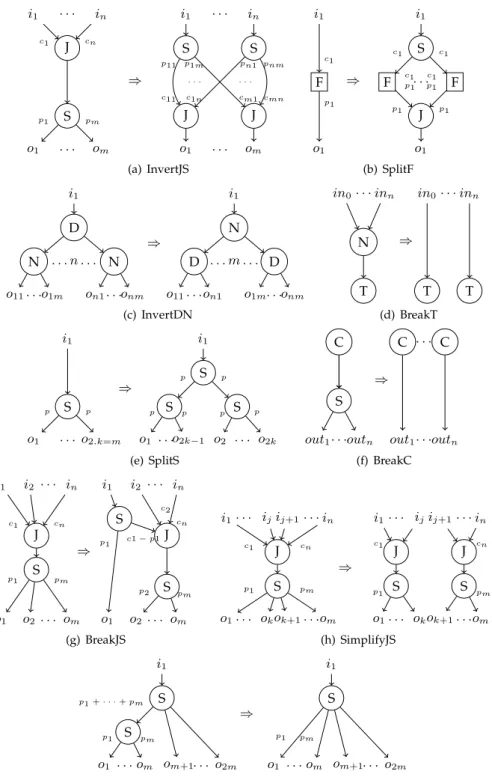
In the following we will describe a set of transformations preserving graph semantics. The match and replacement graphs are given for each transformation in figure 4. The input and output edges are denoted ix and oy in both graphs. The natural correspondence between the ix (resp. oy) of L

and R gives the glue relation. All these transformations are admissible since they satisfy the sufficient conditions stated in lemma 1.

We separate our transformations into two families: transformations and simplifying transforma-tions.

3.2 Transformations

These transformations split or reorder the streams of data and modify the expression of concurrency.

SplitF(fig. 4(b)) This transformation splits a filter on its input. SplitF introduces simple split-join parallelism in the programs. This is legal because filters are pure: we can compute each input block on a different node. The SplitF transformation is parametric in the arity of the split (number of filter nodes used). As splitting a filter once with an arity of 4 or splitting twice with an arity of 2 achieves the same result, splitting is only applied once for any given filter. An already split filter is marked

i1 . . . in o1 . . . om J S c1 cn p1 pm ⇒ i1 . . . in o1 . . . om S S J J pn1 pnm p11 p1m cm1 cmn c11 c1n . . . . (a) InvertJS i1 F o1 c1 p1 ⇒ i1 S J F . . . F o1 c1 c1 c1 c1 p1 p1 p1 p1 (b) SplitF i1 D N . . . n . . . N o11. . .o1m on1. . .onm ⇒ i1 N D . . . m . . . D o11. . .on1 o1m. . .onm (c) InvertDN in0. . . inn N T ⇒ in0. . . inn T T (d) BreakT i1 S o1 . . . o2.k=m p p ⇒ i1 S S S o1 . . .o2k−1 o2 . . . o2k p p p p p p (e) SplitS out1. . .outn C S ⇒ out1. . .outn C . . . C (f) BreakC i1 i2 . . . in o1 o2. . . om J S c1 cn p1 pm ⇒ i1 i2 . . . in o1 o2. . . om J S S c2 cn p1 c1 − p1 p2 pm (g) BreakJS i1. . . ijij+1. . . in o1. . . okok+1. . .om J S c1 cn p1 pm ⇒ i1. . . ijij+1. . . in o1. . . okok+1. . .om J J S S c1 cn p1 pm (h) SimplifyJS i1 S S o1 . . .om om+1. . . o2m p1 pm p1 + · · · + pm ⇒ i1 S o1 . . .om om+1. . . o2m p1 pm (i) SimplifySS

Fig. 4. Set of transformations considered. Each transformation is defined by a graph rewriting rule. Node N denotes a wildcard for any arity compatible node.

InvertJS(fig. 4(a)) This transformation inverts join and split nodes. To achieve this it creates as many split nodes as inputs and as many join nodes as outputs. It then connects together the new split and join stages as shown in the figure. Intuitively, this transformation works by “unrolling” the original nodes (examining consecutive executions of the nodes) so that a common period between the join and split stage emerges. The transformation make explicit the communication pattern in this common period, enabling to invert the join and split stage.

The transformation is admissible in two cases:

1- Each pj is a multiple of C =Pici, the transformation is admissible choosing pij = ci.pj/C, cji= ci. 2- Each ciis a multiple of P =Pjpj, the transformation is admissible choosing pij = pj, cji= pj.ci/P .

Because this transformation exposes the underlying unrolled communication pattern between two computation stages, it may often trigger some simplifying transformations, making the communica-tion pattern simpler or breaking it into independent patterns.

A similar transformation is possible when ∀i, j pi = cj, that is when there is a shuffle between

n input channels and m output channels. We choose not to describe this as a single transformation since it can be achieved using SplitS and SplitJ followed by a RemoveJS.

SplitS / SplitJ(fig. 4(e)) SplitS (resp. SplitJ) creates a hierarchy of split (resp. join) nodes. In the following we will only discuss SplitS. The transformation is parametric in the split arity f . This arity must divide the number of outputs, m = k.f . In the figure, we have chosen f = 2. We forbid the trivial cases (k = 1 or f = 1) where the transformation is the identity. As shown in figure 4(e), the transformation works by rewriting the original split using two separate stages: odd and even elements are separated then odd (resp. even) elements are redirected to the correct outputs.

SplitS and SplitJ can be used together with RemoveJS to break some synchronization points.

InvertDN(fig. 4(c)) This transformation inverts a duplicate node and its children, if they are identical. It is simple to see why this is legitimate. All nodes are pure, their outputs depend only on their inputs; thus applying a process k times to the same input is equivalent to applying the process once making k copies of the output. This transformation eliminates redundant computations in a program.

3.3 Simplifying Transformations

These transformations, remove nodes with either no effect or non-observed computations, and sep-arate split-join structures into independent ones.

SimplifySS / SimplifyJJ(fig. 4(i)) SimplifySS compacts a hierarchy of split nodes. SimplifyJJ is similar for join nodes. We will in the following discuss the SimplifySS transformation. This trans-formation is only possible when the lower split productions sum is equal to the production on the edge connecting the lower and upper splits.

This transformation is useful to put cascades of split nodes in a normal form so that other transformations can operate on them. It should be noted that this transformation is not the inverse of SplitS (breaking the arity of splits instead of the productions sizes).

SimplifyJS(fig. 4(h)) This transformation is possible when the sum of the join consumptions is equal to the sum of the split productions:P

xcx=Pypy. The idea behind this transformation is to

find a partition of the join consumptions and a partition of the split production so that their sum is equal:P

x≤jcx=Py≤kpk. In that case we can split the Join-Split in two smaller Join-Split.

BreakJS(fig. 4(g)) This transformation is very similar to SimplifyJS. It is triggered whenP

xcx=

P

ypybut no partition of the productions/consumptions can be found. In that case the transformation

breaks the edge with the largest consumptions (resp. productions), so that a partition can be found. Both SimplifyJS and BreakJS work on join-splits of the same size. Join-splits of the same size correspond to a periodic shuffle of values. The idea behind these transformations is to make explicit the communications that occur during this shuffle, and separate this communication pattern into independent join-splits when possible.

BreakC(fig. 4(f)) When a constant source is split, we can eliminate the split duplicating the constant source.

BreakT(fig. 4(d)) A node for which all outputs go to a Trash can be replaced by a Trash itself without affecting the semantics. This transformation eliminates subgraphs whose outputs are never observed, it is a kind of dead-code elimination.

RemoveJS / RemoveSJ / RemoveD These transformations are very simple and remove nodes whose composed effect is the identity:

• A join node followed by a split node can be removed if the join productions are the same as

the split consumptions.

• A split node followed by a join node for which the split ithoutput is connected to the join ith

input, both nodes having equal consumptions and productions, can be removed.

• A Duplicate, Join or Split node with only one output branch can be safely removed.

4

E

A

The exploration is an exhaustive search of all the derivations of the input graph using our transfor-mations. We use a branching algorithm with backtracking, as described recursively in algorithm 1. Optimized exploration and exploring a smaller search space are described in Section 4.2.

For this algorithm to terminate we must prove that for every initial graph, once a large enough recursion depth is reached, no transformations will satisfy the for all condition in statement 6. This follows from the fact that the transformations considered cannot produce infinite derivations. This is guaranteed by lemma 2 proved in the next section.

Algorithm 1 EXPLORE(G)

1: Simp ← {SimplifySS, SimplifyJJ, BreakC ...}

2: Tran ← {SplitF, InvertJS, BreakJS, ...}

3: while ∃N ∈ G ∃S ∈Simp such that S applicable at N do

4: G ← SN(G)

5: end while

6: for all N ∈ Gand T ∈ Tran such that T applicable at N do

7: G ← TN(G)

8: EXPLORE(G)

9: end for

10: G ← RESTORE(G)

4.1 Termination

First we define a weight function σ on nodes, then we extend this weight to graphs using a τ function. Finally we introduce a well-founded ordering on the image of τ which we use to prove that no infinite derivation can be generated.

Let us define a weight function σ : Node 7→ N on nodes as:

σ(N ) =        Pn k=1ck if N = J(c1. . . cn) Pm k=1pk if N = S(p1. . . pm) 1 if N = F splitable 0 otherwise

Let τ be a function defined on (Graphs) 7→ (M(N), ≻) as τ (G) = {σ(n) : n ∈ GN odes}. We note

M(N) the set of all finite multisets of N. Since the canonical order on N is well-founded, we can define a well-founded partial multiset ordering ≻ on M(N) [10]. The multiset ordering is defined as follows: ∀M, N ∈ M(N), M ≻ N if for some multisets X, Y ∈ M(N), where X 6= {} and X ⊆ M ,

N = (M − X) ∪ Y and ∀(x, y) ∈ (X, Y ), x > y

That is to say, a multiset is reduced by removing at least one of its elements, and adding any number of smaller elements.

Definition 3: A transformation T is monotone iff G−→ GT ′_{⇒ τ (G) ≻ τ (G}′_{). In words, a}

transforma-tion is monotone if all the weights of added nodes are strictly inferior to the weights of the removed nodes, or if it only removes nodes.

Using the well-foundness of the multiset ordering it is easy to prove the following lemma:

Lemma 2 (Finite derivations): All derivations of a graph G that only make use of monotone

trans-formations are finite.

Computing the weight function for each left-hand side and right-hand side of the graph rewriting transformation shows that all of these transformations are monotone, and termination of algorithm 1 follows.

4.2 Optimizing Exploration

Because the search space is potentially exponential, we have introduced some modifications to the naive exploration presented before.

4.2.1 Dominance rules

Generated graphs G are often obtained through application of transformations operating on distinct part of the graph. In that case, applications of these transformations commute; meaning that the order in which they are applied does not change the resulting graph. Since the order is of no importance, it is more efficient to only explore one of the possible permutations of the application order, and cut the other confluent branches.

To select only one of the possible permutations during our exploration, we introduce an arbitrary ordering (⊏) on our transformations, we say that T1 dominates T2 if T1⊏T₂. A new transformation is applied only if it dominates all the earlier transformations that commute with it.

A sufficient condition for an early transformation T1 to commute with a later transformation T2

is that the nodes that are matched by L2 where already present before applying T1. This condition

can be easily checked if nodes are tagged with a creation date during exploration. 4.2.2 Sandbox exploration

Some data reorganization patterns, like a matrix transposition or a copy of elements, may be modeled with high arity nodes. This is not a problem per se since the complexity of our algorithm is tied to the number of nodes, and not to the number of edges. Yet for some transformations (e.g. InvertJS, InvertND), the number of nodes created is equal to the arity of the original nodes in the matching subgraph. If such transformations are applied to high arity nodes, the complexity explodes. To alleviate this problem, configurations leading to this potential issue are identified.

A node has high arity when it has more than H in or out edges. H can be chosen arbitrarily, H = 30 in our experiments. A graph is compact when all its high arity nodes have a number of distinct children or parents which is less than H. The complexity explosion is caused by transformations that turn a compact graph into a non-compact one. A straightforward approach is to forbid such transformations. Yet this eliminates valuable branches where the graph is compacted shortly after by another transformation.

We would like to forbid the derivations that produce non-compact graphs, yet keeping the deriva-tions in which the graph is compacted shortly after. To achieve this we implement sandbox exploration. The idea of sandbox exploration is to extract high arity nodes along with their close neighborhood. Explore all the derivations of this neighborhood, eliminate all the non compact derivations and keep the compact ones. This optimization eliminates some possible derivations of the search space, making the algorithm non exhaustive. Yet in the applications we have studied, there was little gain in the non-compact derivations that have been removed.

4.3 Partitioning heuristic

Algorithm 1 exhaustive search may take too much time on very large graph instances. The optimiza-tions presented in the previous section, mitigate the problem; nervertheless for really large graphs like Bitonic (370 nodes) or DES (423 nodes) in section 7, the exploration still takes too much time. To deal with very large graph instances we have implemented an heuristic combining our exploration with a graph partitioning of the initial program.

We show that reducing the initial program size, reduces the exploration maximal size. Our heuris-tic, based on this result works by partitioning the initial program.

For this to work, the metrics we optimize must be composable: there must exist a function f that verifies for every partition G1, G2 of G, metric(G) = f (metric(G1), metric(G2)). We will see in

section 6 that the metrics we use to reduce the memory required in a modulo scheduling are indeed composable.

If the metric we try to optimize is composable it is legit to explore each partition separately, selecting the best candidate (which maximizes f ) for each partition, and assemble them back together as detailed in algorithm 2.To partition the graphs we use the freely available Metis [11] graph partitioning tool, trying to reduce the number of edges between partitions.

The downside of this heuristic is that we loose the transformations involving nodes of differ-ent partitions. Yet our benchmarks in section 7 show that the degradation of the final solution is acceptable (except for very small partitions).

Algorithm 2 PARTITIONING(G, P SIZE) 1: n = countN odes(G)

2: p = n/P SIZE

3: partition G in p balanced partitions G1, . . . , Gp

4: for all Gi do

5: EXPLORE(Gi) finds a best candidate Bi

6: end for

7: assemble together the Bi

5

R

M

S

To evaluate our exploration method we have chosen a stream modulo scheduling execution model. We are going to review modulo scheduling in this section, particularly the problem MPA-ii, Memory-constrained Processor Assignment for minimizing Initiation Interval, introduced in [5].

5.1 Mapping and scheduling

In a modulo scheduling each task is assigned a stage. Stages are activated successively, forming a software pipeline. The problem MPA-ii consists in finding a scheduling that reduces the throughput on multiple P E under memory constraints. The solution proposed in [5] uses two separate phases, first they map each node in the graph to a processor, then they assign to each node a pipeline stage.

Let NG be the number of nodes and P the number of PE. For each node i we consider: • aij equal to 1 when node i is assigned to processor j.

• w(i), the work cost of one steady-state execution of the node.

• b(i), the buffer size needed by one steady-state execution of the node. This buffer size depends

of the stage assigned to i which itself depends on the PE mapping. Every node must be assigned to exactly one processor,

P

X

j=1

aij = 1, ∀i = 1, . . . , NG (18)

To optimize the throughput, we balance the cumulated cost in each processor,

NG

X

i=1

w(i).aij ≤ II, ∀j = 1, . . . , P (19)

minimize II (20)

Finally we consider the memory constraint imposed by the available local memory in each PE mem (in this paper we consider that all the PE have the same available memory),

NG

X

i=1

b(i).aij ≤ mem, ∀j = 1, . . . , P (21)

Because the b(i) depends on the mapping the program is not linear. To compute a solution efficiently, the authors in [5] propose the following algorithm:

• Stage1, Make the conservative assumption that all the nodes are assigned to different PE. • Stage2, Assign the earliest possible stages base on the previous assumption.

• Stage3, Compute the b(i) using Stage1 and Stage2.

• Stage4, Solve the ILP problem ((2)+(3)+(4)) using the conservative b(.) of Stage3. • Stage5, Optimize stage assignment based on the PE assignment in Stage4.

5.2 Buffer size

When computing the buffer size needed for implementing the communications over an edge e between node u and node v, the authors in [5] consider two kind of situations:

• u and v are on the same PE, the output buffer of u can be reused by v.

• u and v are on different PE, buffers may not be shared, since a DMA operation d is needed to

transfer the data. The stage in which d is scheduled is noted staged.

The number of elements produced by u and consumed by v on edge e during a steady-state execution is called β(e) and given by eq. (1). Furthermore, since multiple executions of the streams may be on flight in the pipeline at the same time, buffers must be duplicated to preserve data coherency. The number of buffer copies needed depends on the stage difference between the producer u and the consumer v:

δ(u, v) = stagev− stageu+ 1 (22)

The output buffer requirements for all the nodes but Duplicate are, out buf s(i) = X

∀e∈outputs(i)

δ(u, v) ∗ β(e) (23)

For Duplicate nodes, since the output is the same on all the edges, we can share the buffers among all the recipients,

out buf s(i) = max

∀e∈outputs(i)δ(u, v) ∗ β(e) (24)

iff i ≡ D

The input buffer requirements are,

in buf s(i) = X

∀e∈dma inputs(i)

δ(v, d) ∗ β(e) (25) Combining (23)(24)(25) we obtain the total requirements for a node,

b(i) = out buf s(i) + in buf s(i) (26)

6

M

In this section we propose a metric that selects candidates which improve the minimal memory required for the modulo scheduling described in the previous review.

From equations (26)(23)(24)(25) we observe that to reduce the b(i) we can either reduce the stage difference between producers and consumers, δ(u, v), or we can reduce the elements exchanged during a steady state execution, β(e).

The authors of [5] already optimize the δ(u, v) when possible in Stage5. We attempt to reduce b(i) by reducing β(e). To reduce the influence of the β(e) in the buffer cost we search the candidate that minimizes,

maxbuf (G) = max

∀e∈Gβ(e) (27)

if we have a tie between multiple candidates, we chose the one that minimizes, totbuf (G) = X

∀e∈G

β(e) (28)

We note that these metrics are composable, as required by the partitioning heuristic described in sec-tion 4.3. Indeed given a partisec-tion G1, G2of G, we have maxbuf (G) = max(maxbuf (G1), maxbuf (G2))

7

R

We demonstrate the interest of our method in reducing the minimal memory requirements in a modulo-scheduling stream execution model.

7.1 Experimental protocol

We consider a representative set of programs from the StreamIt benchmarks [12]: Matrix Multiplica-tion, Bitonic sort, FFT, DCT, FMradio, Channel Vocoder. We also consider three benchmarks of our own: Hough filter and fine grained Matrix Multiplication (which both contain cycles in the stream graph), and Sobel filter (with high-arity nodes).

We first compute for each benchmark the minimal memory requirements per core for which an

MPA-ii mapping is possible (of course we take into account the optimizations proposed by [5] in

Stage5). We will use this first measure, MPAii mem, as our baseline. We then use our exploration method on each benchmark, and select the best candidate according to the metrics described in section 6. We compute the MPA-ii minimal memory per core requirements for the best candidate: Exploration MPAii mem.

Finally we compute the memory requirements reduction using the following formula: (MPAii mem − Exploration MPAii mem)

MPAii mem

In [4] the authors consider different function splitting variants while solving the ILP of modulo scheduling, yet unlike [5], they do not try to minimize the buffer memory cost. Nevertheless we believe it would be possible to integrate the function split selection described in [4] with the memory constraints of [5]. Thus, to make the comparison fair, we have considered the same function splitting variants when measuring MPAii mem and Exploration MPAii mem. This means that in the results below we do not measure the memory reduction achieved by splitting function blocks (SplitF), we only take into account the memory reduction achieved by the rest of the transformations.

7.2 Memory reduction

The experimental results obtained are summarized in figure 6. The exhaustive search was used when exploring the variants for all the benchmarks except DES and Bitonic for which we used the partitioning heuristic (with PSIZE=60). We achieve a significant memory reduction in seven out of the ten benchmarks. This means in these seven cases we are able to execute the application using significantly less memory than using the approach in [5], therefore we are able to target system with a smaller memory footprint. In terms of throughput, our method does not degrade the performance since we obtain similar II (initialization interval) values than bare MPA-ii.

We can distinguish three categories among the benchmarks:

No effect:DCT, FM, Channel

In this first group of benchmarks, we do not observe any improvement. Indeed these programs make little use of split, join and duplicate nodes. They are almost function only programs. Because our transformations work on data reorganisation nodes, they have no effect on these examples. The very small improvement in Channel is due to a single SimplifyDD that compacts a serie of duplicate nodes.

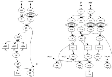
Loop splitting: MM Fine, Hough

These two benchmarks contain cycles. Using our set of transformations we are able to split the cycles, as we demonstrate in figure 5 for the Hough benchmark. This is particularly interesting in the context of modulo scheduling where cycles are fused [4]. As you see in the Hough selected variant, the cycle has been broken in three smaller cycles. Thus after fusion, it has more fine-grained filters, and achieves smaller memory requirements.

Dependencies breaking, and communication reorganisation simplifying: MM coarse, MM fine, FFT, Bitonic, Sobel, DES

The rest of the benchmarks show varying memory reductions. They are due to a better expression of communication patterns. Either non needed dependencies between nodes have been exposed, allowing for a better balancing among the cores, or groups of split, join and dup have been simplified in a less memory consumming pattern.

(a) Original candidate af-ter a SplitF

(b) Best candidate after transformations

1) InvertJS on J6 and S15 2) InvertJS on J16 and S7 3) InvertJS on J8 and S19 4) BreakC on IH 5) RemoveJS on J26 6) InvertJS on J4 and S17 7) InvertDN on D2

(c) The derivation that generated the best candidate, some transformations involve tran-sient nodes that do neither appear in the original graph nor in the best candidate.

Fig. 5. Using our transformations to split cycles on the Hough benchmark.

Bench maxbuf variation totbuf variation

MM fine -1500 -630 MM coarse -1520 -209 Bitonic 0 -480 DES 0 -3514 FFT 0 -184 DCT 0 0 FM -6 +6 Channel 0 -17 Sobel -3392 -3841 Hough -28000 -29933 TABLE 1

Metrics variations between the original graph and the best selected candidate (values represent a number of elements)

7.3 Variation when changing number of PE

In this section we study the memory reduction variance depending on the number of cores in the target architecture. We can identify two categories:

Plateau, graphs in this category, Bitonic, FFT, DES, show little change over the number of PE. We observe in table 1 that for these graphs maxbuf has variated little, but totbuf has decreased.

Bench Exhaustive search time

Search time after partitioning MM fine 2s MM coarse <1s Bitonic >6hours 111s DES 5hours 3.5s FFT 33s DCT <1s FM <1s Channel <1s Sobel 9min18s Hough 3min75s TABLE 2

Fig. 6. Minimal required memory reductions achieved by our proposed method: the results are expressed as a reduction percentage over the minimal required memory per PE obtained by MPA-ii in [5]

Increasing, graphs in this category, MM Fine, MM Coarse, Sobel, Hough, show a better memory improvement the more PEs are used. In table 1 we see that these graphs increase both totbuf and maxbuf .

Graph in category Increasing, break the biggest memory consumer nodes in less greedy nodes. Thus when increasing the number of PE, the mapping algorithm is able to better balance the memory cost since it can split the biggest consumer(s) among multiple processors. This explains that these benches show better results as we increase the PE number. Once we add enough processors to distribute all the new nodes created after the split of the biggest consumer, this increase should stop (we can observe this effect on Hough and MM Fine). In the other hand, the reduction in graphs of category

Plateau, is more uniform, and thus the gain does not depend on the number of PE.

7.4 Exploration cost and Heuristic evaluation

We measure the exploration time of our method for each of the benchmarks. The measures were taken using a Intel Pentium 4 3.8GHz computer with 4Gb of RAM. The exploration algorithms were written in Python and executed using Python 2.5.4 interpreter running on Linux. The results are reported on table 2.

If we do an exhaustive search, exploration times are fast (under 1min) for six of the benchmarks. Sobel and Hough, which possess multiple high-arity nodes, show moderate exploration times (under 10min). Finally, without the heuristic, exploration for DES and Bitonic (the largest benchmarks in our suite) is too long (5 hours for DES; more than 6 hours for Bitonic, we stopped the exploration after that point).

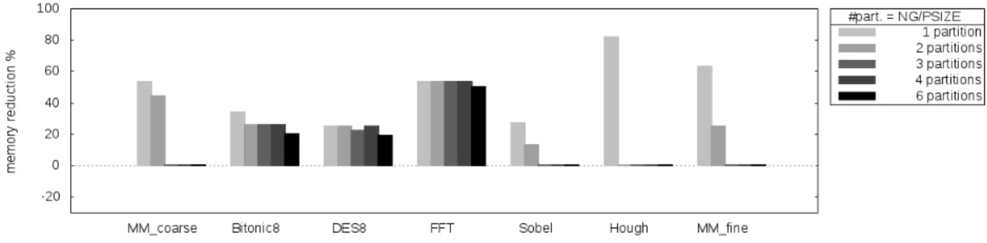
Using the heuristic, with PSIZE=60, the exploration of DES and Bitonic is very fast (under 2min). The partitioning heuristic effectively reduces the running time of these very large graphs, but in the process discards valid transformations. To evaluate the effect of the heuristic on the solution quality, we have compared the memory reduction achieved by the exhaustive exploration to the memory reduction achieved after partitioning the initial graph in 2,3,4 and 6 subgraphs. We have used smaller versions of DES (with 8 mixing stages instead of 16) and Bitonic (with 8 bit strings instead of 32) to evaluate the heuristic (using the original version was impractical because of the very long search time). The results are summarized in figure 7.

The solutions for Bitonic8, Des8 and FFT are quite good even with 6 partitions, they are at most 25% worst than the exhaustive solution.

MM coarse, MM fine, Hough and Sobel, on the other hand, are quickly degraded, and for more than two division do not improve the original program. The extreme degradation of these bench-marks is explained by their small size. Having less than 20 nodes, the partitioning process leaves very small partitions where no transformations are found. The heuristic should be evaluated on larger programs, nevertheless we provide the results for completeness.

8

R

W

Dataflow programming models have been studied for a long time, and many variants have been proposed. Our graphs are defined upon the cyclo-static dataflow model [6] a special case of Kahn process networks [13].

Fig. 7. Evaluation of the partitioning heuristic on 8 PE: for each benchmark, we show the memory reduction achieved when changing NG

P SIZE (the number of partitions used), exhaustive search is

conducted independently in each partition.

The authors of [4] were the first to apply Modulo Scheduling to stream graphs, evaluating their technique on the Cell BE. In [5] their work was extended considering an embedded target with memory and number of PE constraints, MPA-ii is introduced. The authors of [14] successfully used Modulo Scheduling to compile stream graphs on GPU.

The StreamIt project [15], proposes both a stream language, which is very similar to the formalism of our paper, and an optimizing compiler for the Raw [1] architecture. As in our approach, StreamIt adapts the granularity and communications patterns of programs through graph transformation, which it separates in three classes:

• Fusion transformations cluster adjacent filters, coarsening their granularity. • Fission transformations parallelize stateless filters decreasing their granularity.

• Reordering transformations operate on splits and joins to facilitate Fission and Fusion

transfor-mations. The order in which to apply the transformation is decided using a greedy algorithm. We implement Fission transformations on stateless filters using the SplitF transformation. In our approach, Fusion transformations should be delegated to a later clustering phase, since in our case early coarsening would reduce the number of explored variants. Thus we do not use StreamIt fusion transformations during our exploration. Instead, we have concentrated on proposing new Reordering transformations that explore alternate communication patterns. We implement StreamIt filter hoisting on duplicate nodes with InvertND. We propose, through RemoveJS and RemoveSJ, StreamIt syn-chronization removal, which eliminates neighbor split-joins with matching weights. We go further tackling split-join junctions of different weights with InvertJS and BreakJS, eliminating dead-code with BreakT and removing unnecessary synchronization on constant sources using BreakC. To the best of our knowledge StreamIt does not consider reordering transformations on feedback loops. The BreakT transformations which eliminates dead-code was already described in [16].

Array-OL also proposes data transformations in its multi-dimensional dataflow model for signal processing. In Array-OL, the elements that are consumed by a task are defined by successively translating a selection pattern over a multidimensional array. In [17][18] the authors show that in some cases it is possible to share the patterns for two succesive tasks. We achieve a similar effect on our model using InvertDN, indeed if two function nodes work on similar patterns there is a chance that our transformations exposes the common pattern as a number of common subgraphs under a Duplicate node; using InvertDN we are able to hoist the common pattern over the duplicate node.

Dataflow transformations approaches have been proposed to optimize circuit design [19][20], but they usually target a much smaller granularity of nodes than our filters.

Many methods for optimizing CSDF multiprocessor schedules have already been proposed, some concentrate on maximizing the throughput [6][21], other on minimizing the memory requirements [22] and some search best pareto configurations for both criteria [23]. Our approach does not act at the schedule level but at the implementation level, it is therefore complementary to these approaches which operate on the schedule.

9

C

We propose a design space exploration to reduce memory requirements of stream programs un-der modulo scheduling. Memory reduction is achieved through succesive semantically preserving

transformations, that break cycles, break dependencies and simplify communication patterns in the stream graph.

We propose an efficient heuristic to explore the different transformations combinations based on graph partitioning. We demonstrate the interest of the approach on a significant panel of benchmarks. We think that this approach is flexible and could also be used with a different metric to adapt stream programs to other constraints as communication bus capacities, maximum latencies, memory hierarchies. We plan to investigate this in the future.

R

[1] M. I. Gordon, W. Thies, M. Karczmarek, J. Lin, A. S. Meli, A. A. Lamb, C. Leger, J. Wong, H. Hoffmann, D. Maze, and S. Amarasinghe, “A stream compiler for communication-exposed architectures,” in Intl. Conf. on Architectural Support for Programming Languages and Operating Systems. ACM, 2002.

[2] T. Goubier, F. Blanc, S. Louise, R. Sirdey, and V. David, “D´efinition du langage de programmation ΣC, RT CEA LIST DTSI/SARC/08-466/TG,” Tech. Rep., 2008.

[3] C. Aussagu`es, E. Ohayon, K. Brifault, and Q. Dinh, “Using multi-core architectures to execute high performance-oriented real-time applications,” to appear in proc. of Int. Conf. on Parallel Computing, 2009.

[4] M. Kudlur and S. Mahlke, “Orchestrating the execution of stream programs on multicore platforms,” in PLDI ’08: Proceedings of the 2008 ACM SIGPLAN conference on Programming language design and implementation. New York, NY, USA: ACM, 2008, pp. 114–124.

[5] Y. Choi, Y. Lin, N. Chong, S. Mahlke, and T. Mudge, “Stream compilation for real-time embedded multicore systems,” in International Symposium on Code Generation and Optimization. Washington, DC, USA: IEEE Computer Society, 2009, pp. 210–220.

[6] G. Bilsen, M. Engels, R. Lauwereins, and J. Peperstraete, “Cycle-static dataflow,” IEEE Trans. on Signal Processing, vol. 44, no. 2, pp. 397–408, Feb 1996.

[7] E. A. Lee and D. G. Messerschmitt, “Static scheduling of synchronous data flow programs for digital signal processing,” IEEE Trans. Comput., vol. 36, no. 1, pp. 24–35, 1987.

[8] M. Andries, G. Engels, A. Habel, B. Hoffmann, H.-J. Kreowski, S. Kuske, D. Plump, A. Sch ¨urr, and G. Taentzer, “Graph transformation for specification and programming,” Sci. Comput. Program., vol. 34, no. 1, pp. 1–54, 1999.

[9] P. Panangaden and V. Shanbhogue, “The expressive power of indeterminate dataflow primitives,” Information and Computation, vol. 98, pp. 99–131, 1992.

[10] N. Dershowitz and Z. Manna, “Proving termination with multiset orderings,” Comm. ACM, vol. 22, no. 8, pp. 465–476, 1979.

[11] G. Karypis and V. Kumar, “A fast and high quality multilevel scheme for partitioning irregular graphs,” SIAM J. Sci. Comput., vol. 20, no. 1, pp. 359–392, 1998.

[12] “Streamit benchmarks,” http://groups.csail.mit.edu/cag/streamit/shtml/benchmarks.shtml.

[13] G. Kahn, “The semantics of a simple language for parallel programming,” in IFIP Congress, J. L. Rosenfeld, Ed. New York, NY: North-Holland, 1974, pp. 471–475.

[14] A. Udupa, R. Govindarajan, and M. J. Thazhuthaveetil, “Software pipelined execution of stream programs on gpus,” in Int. Symp. on Code Generation and Optimization. Washington, DC, USA: IEEE Computer Society, 2009, pp. 200–209. [15] W. Thies, M. Karczmarek, and S. P. Amarasinghe, “StreamIt: A Language for Streaming Applications,” in Proc. of the Intl.

Conf. on Compiler Construction, 2002.

[16] T. M. Parks, J. L. Pino, and E. A. Lee, “A comparison of synchronous and cycle-static dataflow,” in Asilomar Conf. on Signals, Systems and Computers. Washington: IEEE Computer Society, 1995, p. 204.

[17] A. Amar, P. Boulet, and P. Dumont, “Projection of the Array-OL specification language onto the kahn process network computation model,” in Intl. Symp. on Parallel Architectures, Algorithms and Networks. Washington, DC, USA: IEEE Computer Society, 2005, pp. 496–503.

[18] J. Soula, “Principe de compilation d’un langage de traˆıtement de signal,” Ph.D. dissertation, Universit´e de Lille, Lille, France, 2001.

[19] A. Chandrakasan, M. Potkonjak, J. Rabaey, and R. Brodersen, “An approach for power minimization using transforma-tions,” Oct 1992, pp. 41–50.

[20] A. K. Verma, P. Brisk, and P. Ienne, “Data-flow transformations to maximize the use of carry-save representation in arithmetic circuits,” IEEE Trans. on CAD of Integrated Circuits and Systems, vol. 27, no. 10, pp. 1761–1774, 2008.

[21] J. Falk, J. Keinert, C. Haubelt, J. Teich, and S. S. Bhattacharyya, “A generalized static data flow clustering algorithm for mpsoc scheduling of multimedia applications,” in ACM Intl. Conf. on Embedded Software. Atlanta: ACM, 2008, pp. 189–198.

[22] M. Wiggers, M. Bekooij, and G. Smit, “Efficient computation of buffer capacities for cyclo-static dataflow graphs,” in Conf. on Design Automation. San Diego, California: ACM, 2007, pp. 658–663.

[23] S. Stuijk, M. Geilen, and T. Basten, “Throughput-buffering trade-off exploration for cyclo-static and synchronous dataflow graphs,” IEEE Trans. Comput., vol. 57, no. 10, pp. 1331–1345, 2008.