The Impact of Branch Prediction on Control Structures for Dynamic Dispatch in Java

HAL Id: inria-00072041

https://hal.inria.fr/inria-00072041

Submitted on 23 May 2006

HAL is a multi-disciplinary open access

archive for the deposit and dissemination of

sci-entific research documents, whether they are

pub-lished or not. The documents may come from

L’archive ouverte pluridisciplinaire HAL, est

destinée au dépôt et à la diffusion de documents

scientifiques de niveau recherche, publiés ou non,

émanant des établissements d’enseignement et de

The Impact of Branch Prediction on Control Structures

for Dynamic Dispatch in Java

Dayong Gu, Olivier Zendra, Karel Driesen

To cite this version:

Dayong Gu, Olivier Zendra, Karel Driesen. The Impact of Branch Prediction on Control Structures

for Dynamic Dispatch in Java. [Research Report] RR-4547, INRIA. 2002, pp.12. �inria-00072041�

INSTITUT NATIONAL DE RECHERCHE EN INFORMATIQUE ET AUTOMATIQUE

The Impact of Branch Prediction on Control

Structures for Dynamic Dispatch in Java

Dayong Gu

−

Olivier Zendra

−

Karel Driesen

N°4547

Septembre 2002



THEME 2



ISRN INRIA/RR--4547--FR+ENG

a p p o r t

d e r e c h e r c h e

The Impact of Branch Prediction on Control Structures

for Dynamic Dispatch in Java

Dayong Gu

−

Olivier Zendra

−

Karel Driesen

Thème 2

−

Génie Logiciel et calcul symbolique

Projet MIRO

Rapport de recherche n° 4547

−

Septembre 2002

−

12 pages

Abstract: Dynamic dispatch, or late binding of function calls, is a salient feature of object-oriented

programming languages like C++ and Java. The target of a dispatched call changes according to the type of

the object receiving the call. Due to inheritance the exact type is unknown at compile time, and therefore

dispatch must occur in general at run time, implying a cost to the use of object-oriented programming

languages. In previous work, we measured the performance of various equivalent non-object-oriented control

structures to determine if dispatch cost can be reduced by translation. Measurements on a variety of virtual

machines and hardware platforms show that alternative control structures are useful for a low number of

expected types (low degrees of polymorphism). However, the gains differ substantially for different type

patterns, even when the number of types is constant. The difference is likely to be caused by a processor's

branch predictor, which guess the outcome of branches involved in dynamic dispatch .In this paper, we

simulate branch predictors of Athlon and Pentium in order to validate this insight. The results show that

branch prediction accuracy is indeed responsible. For successful optimization it is therefore not sufficient to

guess the number of types occurring in a call. The type pattern should also be taken into account.

Key-words: Java, dynamic dispatch, object-oriented, control structure, branch prediction

Ce travail de recherche fait suite au postdoctorat INRIA d'Olivier Zendra à McGill University.

Egalement publié comme Technical Report SOCS-02.6, School Of Computer Science, McGill University.

Dayong Gu est membre de l'Adaptive Computation Lab de McGill University, Montréal, Canada.

Karel Driesen est professeur à McGill University, Montréal, Canada, et responsable du laboratoire ACL.

Unité de recherche INRIA Lorraine

LORIA, Technopole de Nancy-Brabois, Campus Scientifique,

615 rue du Jardin Botanique, BP 101, 54602 Villers-Lès-Nancy (France)

Impact de la prédiction de branchement sur les

structures de contrôle pour la liaison dynamique en Java

Résumé: La liaison dynamique, ou envoi de messages, est un concept saillant dans les langages à objets

comme C++ et Java. Java. La cible d'un envoi de message change en fonction du type de l'objet receveur. A

cause de l'héritage, ce type exact n'est pas connu lors de la compilation; une liaison dynamique doit donc être

effectuée dans le cas général lors de l'exécution, ce qui implique un coût supplémentaire lors de l'utilisation

de langages à objets. Dans nos précédents travaux, nous avons mesuré la performance de diverses structures

de contrôles classiques équivalentes, afin de déterminer si le coût de la liaison dynamique peut être réduit en

les utilisant. Nos expériences, sur diverses machines virtuelles et plateformes matérielles, montrent que ces

structures de contrôle alternatives sont utile lorsque le nombre de types attendus est faible (faible degré de

polymorphisme). Néanmoins, les gains varient largement selon les différent patterns de types, même quand

le nombre de types est constant. Ces différences sont probablement causées par les prédicteurs de

branchement des processeurs, qui prédisent le résultat des branchements impliqués dans la liaison dynamique.

Dans ce document, nous simulons les prédicteurs de branchement de l'Athlon et du Pentium afin de valider

cette hypothèse. Nos résultats montrent que la précision de la prédiction est en effet responsable. Pour

optimiser efficacement, il n'est donc pas suffisant de prédire le nombre de types possibles pour le receveur.

Le pattern des types doit aussi être pris en considération.

The Impact of Branch Prediction on Control Structures

for Dynamic Dispatch in Java

Dayong Gu

Adaptive Computation Lab, McGill University, Canada

[email protected]

Olivier Zendra

INRIA-Lorraine / LORIA, France

[email protected]

Karel Driesen

Adaptive Computation Lab, McGill University, Canada

[email protected]

Abstract

Dynamic dispatch, or late binding of function calls, is a salient feature of object-oriented languages like C++ and Java. The target of a dispatched call changes according to the type of the object receiving the call. Due to inheritance the exact type is unknown at compile time, and therefore dispatch must occur in general at run time, implying a cost to the use of object-oriented programming languages. In previous work, we measure the performance of various equivalent

non-object-oriented control structures to

determine if dispatch cost can be reduced by translation. Measurements on a variety of virtual machines and hardware platforms show that alternative control structures are useful for a low number of expected types (low degrees of

polymorphism). However, the gains differ

substantially for different type patterns, even when the number of types is constant. The difference is likely to be caused by a processor’s branch predictor, which guesses the outcome of branches involved in dynamic dispatch.

In this paper, we simulate branch predictors of Athlon and Pentium in order to validate this insight. The results show that branch prediction accuracy is indeed responsible. For successful optimization it is therefore not sufficient to guess the number of types occurring in a call. The type pattern should also be taken into account.

Keywords:

dynamic dispatch, Java, object-oriented, branch prediction, control structure

1

Introduction

Dynamic dispatch is a salient feature of object-oriented programming languages like C++ and Java. When a virtual method call in Java is executed, the object that receives the call retrieves the class-specific method implementation and invokes it. This late binding of dispatch targets allows any object to play the role of the receiver object, as long as the new object implements the expected interface (it is substitutable à la Liskov [7]). Such type-substitutability enables better code abstraction and code-reuse, and is therefore one of

the main advantages of object-oriented

programming languages.

Consequently, dynamic dispatch occurs

frequently. For instance, virtual method

invocations in Java [4] occur every 12 to 40 byte codes [2]).

Unfortunately, virtual method calls can be very time-consuming. The main cause of their inefficiency is the indirect branch instruction that resides at the core of a virtual method call. On

modern, deeply pipelined processors,

mispredicted indirect branches cause “pipeline bubbles” which stall the CPU [3].

One possible optimization translates the call to a non-object-oriented control structure (e.g. if

sequence), in the expectation that it will be

compiled into less expensive native code

instructions. We explored this strategy in [11], using real time measurements of four groups of benchmarks running on various run time type patterns, on a several virtual machines and different hardware platforms. We found that a

translation to non-object-oriented control

structures reduces execution time for dynamically dispatched calls with few types. However, the gain depends highly on the type pattern, which led to the hypothesis that mispredictions of the branch predictor are responsible for this difference.

In this study, we simulate the branch

predictors of an Athlon and Pentium III processor in order to determine the influence of branch prediction on the efficiency of control structures for dynamic dispatch.

The paper is organized as follows. In section 2, we present the methodology, both of the original real time experiment and the simulation executed in this paper. In section 3 we present and discuss the results. The last two sections conclude and mention future work.

2

Methodology

Figure 1 compares the structure of the real

time experiment in [11] and the current

experiment, based on simulation:

Figure 1: Structure of the experiments

The real time experiment simply consists of running the benchmarks on Sun’s Hotspot JVM 1.3 and recording the execution time (see section 2.1 for benchmark descriptions). In this study we only consider one virtual machine and two platforms based on the same x86 instruction set

architecture, to factor out differences in

compilation and ISA. We found in [11] that results were determined primarily by the hardware platform and that execution trends differed little

between different JVM’s. For the simulation

experiment we first executed the benchmark using an instrumented Kaffe (1.0.6) JVM, which provided byte code execution traces for the inner loop of the benchmarks. These traces were then offered to the Plumber. Plumber is a branch prediction simulator designed to count branch prediction misses for a variety of different architectures. The aim of the experiment was to obtain cost estimates close to the real time measurements, using a simple cost calculation model at the byte code level which takes into account branch prediction at the processor level.

2.1 Benchmark programs

We designed the micro benchmarks in order to emphasize the cost of one dynamically dispatched call under a variety of run time execution conditions. Figure2 shows an overview of all benchmark programs. They share the same structure, executing a loop in which a static function is called on an object extracted from an array (the array is initialized to a particular type pattern from a file; we show the type ID’s). The static function differs according to the control structure which we want to measure.

Figure 2: Benchmark programs

Benchmarks Hotspot 1.3.1

Pentium III

Hotspot 1.3.1 Athlon

Real time result

Kaffe JVM

Simulated result Byte Code execution Traces

Pentium III Branch Predictor Simulation in Plumber Athlon Branch Predictor Simulation in Plumber 10₀ 0 0 1 | 5 | 3 | 4 | 3 | 2 | 1 | 4 | 5 | 2 | 4 | 3 | 1 … Pattern array Loop : i = 0 to loopNum

Func(array[i])

Benchmarks were generated for different

static type sizes (number of types that can

occur):

.

"Virtual invocation":

In this group, all the benchmark programs have one virtual method call site in a large loop. The number of possible types is different for different benchmark programs. However, the core code sequence remains the same:

p.foo(x);

.

"If-Sequence":

If-sequence benchmarks use a sequence of 2-way conditional type checks to determine the call target. The size of this structure is determined by the number of possible types. The code below demonstrates the core code sequence for a call with 4 possible types:

int localId = p.typeID; if (localId == ID_1 )

Class1.foo_static(x);

else if (localId == ID_2 )

Class2.foo_static(x);

else if (localId == ID_3 )

Class3.foo_static(x);

else // localId == ID_4

Class4.foo_static(x);

.

"Binary Tree":

Binary tree benchmarks are similar to if-sequences, but use inequality and are organized as a binary decision tree. The depends on static type size. The core code sequence for four types:

int localId = p.typeID; if (localId <= ID_2) if (localId <= ID_1) Class1.foo_static(x) else Class2.foo_static(x) else if (localId <= ID_3) Class3.foo_static(x) else Class4.foo_static(x);

.

"Switch":

Switch benchmarks were measured in [11]. They use as core code sequence a dense Java switch statement. Their behavior depends on the virtual machine used. For instance, for the Hotspot JVM, they behave as if-sequences, for the IBM JVM, they behave as virtual function calls.

We therefore did not include them in this study, as their behavior in terms of branch prediction is explained by the corresponding if-sequence or virtual function call behavior.

.

"NoCall":

NoCall benchmarks are used as baseline, to estimate benchmark overhead: execution time of all byte codes except those involved in dynamic dispatch. We took care to ensure that the compiler was not able to optimize away this overhead.

In order to factor out differences in generated

code sequences, we focus on benchmark

programs which have 20 possible types. In [11] we measured the effect of different static type sizes.

2.2 Type patterns

In order to measure the effect of different type execution patterns while ensuring that a smart compiler can not guess their occurrence, the array in figure 2 is initialized from a pattern file. Each number causes an object of a particular type to be allocated and store in the pattern array. We use four sets of pattern files in the experiment:

.

Const Patterns:

A particular const pattern file is a sequence of one particular integer:

cst_01: 1,1,1,1,1,1,1,1… cst_02: 2,2,2,2,2,2,2,2… cst_03: 3,3,3,3,3,3,3,3…

These patterns represent a 100% monomorphic case (no changes in type, and therefore the call always dispatches to the same target).

.

Cyclic Patterns:

Cyclic patterns cycle through a range of types:

cycl-02: 1,2,1,2,1,2,1,2,1… cycl-03: 1,2,3,1,2,3,1,2,3… cycl-04: 1,2,3,4,1,2,3,4,1…

.

Random Patterns :

Random patterns exercise an unpredictable variation of types within a certain range:

rnd-03: 1,2,2,2,3,2,3,1,3,3,1… rnd-04: 1,2,4,3,2,3,1,4,2,3,2… rnd-05: 2,5,4,1,3,3,5,1,4,4,1…

Step patterns exercise a range of types with as few changes as possible within a pattern file:

step-02: 1,1,1,1,…,1,…,2,2,2,…,2 step-03: 1,1,…,1,2,2,…,2,3,3,…,3

For each of the three variational patterns we test the range 01-02 up to 01-10 and 01-20. For the constant pattern we test the values 01 to 10 and 20. This gives 41 data points for each benchmark program.

3

Motivation

3.1 Real time results

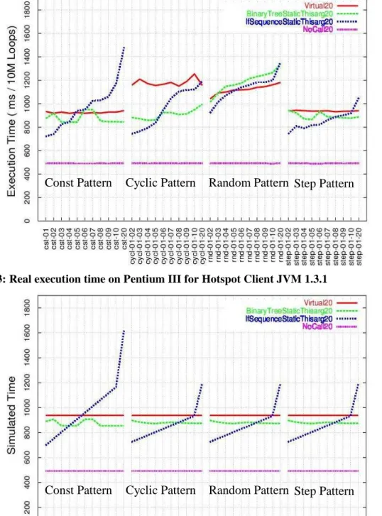
Figure 3 shows the real time execution cost in ms per 10 million loops, of the 41 patterns on each benchmark program, running under the Hotspot JVM on a Pentium III. The following observations from [11] also hold for other JVM’s and platforms:

.

The performance of dynamic dispatch (red

curve Virtual20) can be significantly improved by

translation to equivalent non-object-oriented

control structures for virtual calls with a small number of possible receiver types. Binary trees

(green curve BinaryTreeStaticThisarg20) are

significantly faster than virtual calls for cyclic

patterns. If-sequences (blue curve

IfSequenceStaticThisarg20) are faster if the

number of types is small (< 5).

.

The performance depends substantially on

the run time execution pattern. For example, for 10 different types, the cyclic (cycl-01-10) and step

patterns (step-01-10) exhibit very different

execution times for virtual calls and if sequences, even though they both touch the same number of types an identical number of times. Only the order in which types are encountered differs.

3.2 Simulated results without

branch prediction misses

In order to isolate the dependence of execution time on execution pattern, we compare the execution times in figure 3 with the simulated execution times in figure 4. The estimates do not yet take into account branch prediction misses, but simply count the number of byte codes executed (see Section 4 for exact cost formulas).

For the constant pattern, simulated execution times approximate real times closely. The if

sequence cost rises linearly with the type number

since higher numbered types are located further back in the sequence. For example, the cst-01 pattern always matches the type tested in the first if statement of the sequence, while the cst-10 pattern traverses ten ifs before a match is found. The binary tree program is fairly constant since all types are found at the leaf of the tree. For a static type size of 20, 4 to 5 if statements are executed. The slight variation for patterns cst-02, cst-06 and cst-07 occurs because these patterns are located one level deeper than the other types, and therefore execute one extra if statement.

Virtual function calls for constant type patterns

are about as fast as binary trees.

Since the simulation only counts the number of byte codes executed, it predicts identical execution times for the step pattern, cyclic pattern and random pattern. Of these three, only the step

pattern corresponds well to real execution timings. Apart from a few spurious bumps, simulation neatly duplicates the trends of

if-sequence, binary tree and virtual function call. In

contrast, both the cyclic pattern and the random

pattern exhibit significantly higher real execution

times than estimated.

Why do the execution times of these patterns differ so much? Since all three patterns execute the same number and type of byte codes and therefore the same number and type of native code instructions, the answer to this question can only include caching and branch prediction effects. Since the code sequences are small enough to fit into the instruction cache, and since the data access pattern is identical for all patterns (step through the pattern array), instruction or data cache misses can not be responsible. Therefore

branch prediction misses must be the cause of the

higher cost of cyclic and random patterns as compared to step patterns. Since the step pattern exhibits very few changes in the type offered to dispatch control structures, very few changes in branch direction occur during a complete run. The Pentium III branch predictor therefore accurately predicts branch targets, and the simulation, which assumes a constant cost for all statements accurately estimates real execution times.

Having established the importance of branch prediction in the execution cost of cyclic and

random patterns, we model and simulate the

Pentium III and Athlon branch prediction

architectures in the next section.

Figure 3: Real execution time on Pentium III for Hotspot Client JVM 1.3.1

Figure 4: Simulated execution time on Pentium III without branch prediction misses

Const Pattern

Cyclic Pattern

Random Pattern Step Pattern

4

Simulation

In this section we discuss in detail the simulation scheme used to obtain our results.

4.1 Trace based simulation

Our simulation is driven by byte code execution traces of the benchmark programs presented in section 2, for static type size 20. We instrumented the Kaffe Java Virtual Machine to generate information for each executed byte code. For most byte codes we simply generate the byte code number, and the location of the

byte code, encoded as a 64 bit “PC” (32-bit

class ID, 16-bit method ID, 16 bit method offset). For byte codes that transfer control such as those generated by if statements (if_icmpne,

if_icmple and ifgt), and method calls

(invokevirtual) we also generate the target PC. Note that this encoding abstracts away from many implementation details. In effect, we ignore all compiler and processor instruction set architecture issues. The correspondence between figure 3 and figure 4 for constant and step patterns validates this approach: our simulation

captures the crucial aspects of execution

overhead of dispatch control structures.

Since our focus is on the long running loop executing the dynamically dispatched call, we do not need to trace the complete benchmark. It would also not be practical to do so since the resulting trace file would take up 27GB of disk space per data point. Therefore we trace only a fragment of the execution, making sure that we capture a complete run through the pattern array

depicted in figure 2. After 50 million byte

codes, tracing is switched on for the next 400000 byte codes, resulting in a manageable 10MB trace file per data point.

4.2 Branch prediction

The Plumber package [8] is a framework written in Java for simulating different predictor architectures and measuring prediction rates. Plumber reads the byte code traces generated by Kaffe, counts the number of byte codes executed, and predicts the targets of if statements and invokevirtuals, assuming that every if statement translates to a conditional branch, and every invokevirtual to an indirect branch, as is the case in most current JVM’s.

4.2.1 Athlon Branch Predictor

The Athlon processor uses a 2-bit counter GAS predictor with 8 bit global history to make a “taken/not taken” prediction for conditional branches. The Branch History Table has 4096 entries. It concatenates 8 bits history and 4 bits from the branch address to a 12 bit key pattern for the Branch History Table. Indirect branch targets are predicted by the Athlon predictor using a 2048 entry Branch Target Buffer which stores the most recent target address [6]. A branch whose target is predicted incorrectly incurs a penalty of minimum 10 cycles[1].

Figure 5 shows the structure of the Athlon GAS predictor.

Figure 5 Athlon GAS predictor

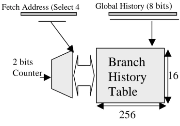
4.2.2 Pentium III Branch Predictor

The Pentium III processor uses a 512-entry Branch Target Buffer to store branch targets for

conditional and indirect branches. For

conditional branches, the BTB also stores a 4 bit local taken/not taken history. This history is associated with a 16-entry per-branch table which stores two bit counters to predict the

branch direction. The Pentium therefore

implements the PaP two-level predictor scheme [9,10]. If there is no valid entry in the BTB for a branch, a static predictor provides a prediction based on the direction of the branch (backward-taken/forward-not-taken). A branch whose target is predicted incorrectly incurs a penalty between 10 and 15 cycles and possibly as many as 26 cycles [5].

Fetch Address (Select 4 Global History (8bits)

Branch

History

Table

2 bits Counter

256

16

4.2.3

Differences between real

and simulated predictors

Since the traces are based on byte codes, we do not have information on the actual addresses (PC) manipulated by the branch predictors. For instance, the Athlon predictor uses 4 bits from the 32-bit address of an instruction as part of the key pattern. The traces do not contain physical addresses. Instead they contain a 64 bit PC which uniquely identifies a target byte code. In order to obtain 4 bits with similar variation as 4 lower order bits of physical addresses we fold the 64-bit address into 4 bits by repeatedly XOR-ing every 4-bit chunk of the address. Therefore our simulator does not model interference misses in the branch predictor table. Since interference misses can change even for identical processors and programs if the program is relocated in memory we felt justified in ignoring them in our simulations. For the Pentium, a similar operation transforms the 64-bit address into the 9 bits used to obtain a branch entry in the branch target buffer.

4.3 Cost estimation

The branch prediction simulator gives us the average number of branch prediction misses Nm, the number of byte codes executed N, and the number of invoke virtual byte codes executed

Nv (1 or 0) per dynamically dispatched call.

The cost of one execution of a dispatch call control structure is then estimated as:

CallCost = (Nm*P + N + Nv*V) * T (1)

where:

Nm*P

the branch misprediction cost

P = branch penalty in byte code units N

the cost of byte codes in the call all except invoke virtual have unit cost

Nv*V

the cost of invoke virtual byte codes

V = cost of one invoke in byte code units T

a processor-specific constant which scales the call cost in byte code unit cost to a real time value in ms.

P, V and T are calculated from the real time

measurements. The real time measurement is

modeled by the following formula:

CallCost * NumberOfLoops + NoCallCost (2) where:

NumberOfLoops

the number of times the loop in figure 2 is executed

NoCallCost

the real time measurement of the benchmark executing no calls, which includes all loop overhead

Formula (2) allows us to extract the portion of real time execution cost that is due to byte codes executed for the dispatch control structure, since this is the only difference between regular benchmark programs and the NoCall benchmark. Once we have the CallCost, the processor-specific constant T can be calculated from the

real time measurement of the if-sequence

benchmark on const patterns, since Nm and Nc are 0 (no branch prediction misses for a const

pattern, no invoke virtual for an if sequence),

and N is counted by the simulator, so that:

CallCostcst-01= (N) * Tcst-01

After we obtain the value of T, we can calculate the cost of invoke virtual byte codes V from the real time measurement of the virtual

invocation benchmark on the step patterns. Since

both the Athlon and the Pentium III store the last target of the invoke virtual as an indirect branch target in their respective Branch Target Buffers (BTB), the number of branch prediction misses

Nm is close to 0 (for step-02, Nm = 2/10000).

Formula (1) therefore reverts to:

CallCoststep-02= ( N + 1*Vstep-02) * T

After we obtain the value of V, the only unknown quantity is the branch penalty P in byte

code unit cost. An approximate value is

calculated from the virtual invocation

benchmark on cyclic patterns where a BTB

mispredicts every time (Nm = 1). Formula (1) then becomes:

CallCostcycl-02= (1*Pcycl-02+ N + 1*V) * T

The values obtained for both processors are: 733MHz Pentium: T =1.73 E-6 V =21.8 P =14.0

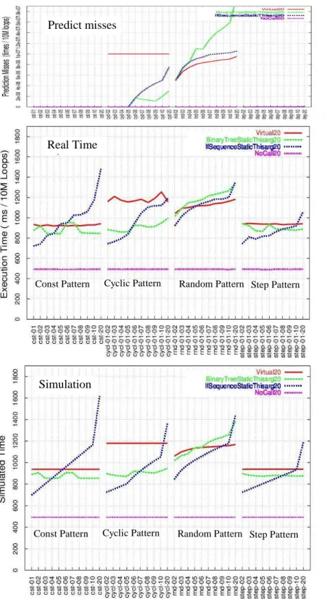
Figure 6: The misses, real and simulated execution time on Pentium III

Predict misses

Real Time

misses

Simulation

Const Pattern Cyclic Pattern Random Pattern Step Pattern

Figure7: The misses, real and simulated execution time on Athlon

Predict Misses

Real Time

Simulation

Const Pattern Cyclic Pattern Random Pattern Step Pattern

5

Results

Based on the number of mispredictions in the simulated predictor, the total number of byte codes executed in the 10,000 loops in the trace file and the simulated execution time calculated by the formulae in 4.3, we generated the graphs in figure 6 and 7. The Y-axis represents time for the

graphs on real execution time, simulated

execution time for the simulation graphs and number of branch prediction misses for the predict miss graphs. The red, green, blue and purple curves are for the Virtual, Binary Tree, If-Sequence and NoCall benchmarks, respectively.

In figure 6 we repeat the result of the real time measurement experiment of [11] on a 733 MHz Pentium III running the HotSpot JVM 1.3.1, whereas the result of the same experiment on a 1.4GHz Athlon processor is shown in figure 7.

5.1 Real and simulated results

comparison

The number of executed byte codes is the main determining factor for the run time execution cost of the benchmarks. Figure 4 shows the simulated execution time on Pentium III without the impact of the misprediction. In other words, in this graph we consider the predictor perfect, as discussed in section 4.

Figure 6, for Pentium III, and figure 7, for Athlon, both comprise three graphs each. The smaller graph on top shows the misses for the benchmarks on the simulated predictor for the corresponding processor. The graph in the middle is the real results (for figure 7, it is the same as figure 3), whereas the bottom graph shows the simulated results including branch misprediction penalties.

Overall, the shapes of the curves in the simulated results are very similar to those in the real results, except for some irregular small bumps in the latter which we believe are caused by artifacts such as address interference in branch prediction tables or instruction cache, which the simulation does not model.

In the following three sections, we discuss in detail the results for each of the three benchmarks

programs1.

1_{NoCall being a baseline, it is not studied per se.}

5.2 Virtual Benchmark

The number of executed byte codes of the Virtual benchmark across all the patterns (the X-axis) are the same, as shown by figure 4.

However, the real execution time of this benchmark on different patterns varies quite a lot, especially for the Pentium III (figure 3). The curves for the Virtual benchmark (red) on the

constant and step patterns are much lower than

the other two curves (with the step pattern curve being slightly above the one for the constant pattern), which indicates a shorter execution time. The curve corresponding to the cyclic patterns has a shape similar to that of the constant and step curves, that is, almost a straight line. The curve for the random patterns shows a slight, monotonous increase, which reaches its highest point at the far right (random20), with a value similar to that of the cyclic curve.

The graphs for branch mispredictions (top graphs) explain most of these observations.

The fact there are no misses in the constant and step patterns explains their lower execution time compared to cyclic and random.

When a random pattern is considered, the misprediction rate increases with the number of different types occurring in the pattern. For example, when only two types occur in random order, a Branch Target Buffer that stores the last target of the call will predict the right target 50% of the time. Average prediction accuracy goes down as 1/number of types. Branch prediction misses therefore explain the increase of the red curve in the top graphs of figures 6 and 7, with the higher value being the rightmost one (20), where the misprediction rate becomes similar to that of the cyclic curve. This corresponds to the shapes seen in the graphs for the real execution time.

In the bottom graphs for the simulated execution times, that take into account the mispredictions, the four red curves have shapes and levels very similar to those of the real time curves.

5.3 Binary Tree Benchmark

First of all, the shape of the curves for the Binary Tree benchmark (green) on the constant patterns and the step patterns are very similar, when looking at the graphs for real execution time, simulated time and at figure 6. Furthermore, the mispredictions of these two groups of patterns are zero, as shown on the top graphs of figures 6

and 7. As a consequence, the execution times are determined mainly by the number of executed byte codes.

Secondly, the shape of the green curves for the

cyclic and random patterns in the real time graph

are very different from those in figure 4, which assumes no misprediction. While the curves in figure 4 are in fact almost flat lines, the real time curves go up and down. Their overall trend is similar to the shape of the curves in the graphs for mispredictions.

Let us use the curves for the cyclic patterns as an example. The two green curves, cyclic for real time (middle graphs) and cyclic for misses (top graphs), begin as a flat line for one to five

possibilities, and then suddenly go up

significantly from the point for the cyclic--06 pattern. After that point, they go down smoothly until the point for the cyclic-09 pattern is reached, and then they go up again.

Similar observations can be made for the curves in these two real time graphs and misprediction graphs for the random patterns. Not only are the shapes similar, but also the relative values when compared to other curves. For example, the lowest points of the curves for the

random patterns (leftmost points) are both higher

than those of the cyclic patterns, in the two graphs (top and middle) of the figure for each processor (figure 6 and 7).

In the simulated execution time graphs, the green curves for the Binary Tree benchmark have a shapes and positions that are similar to those of the corresponding curves ones in the real time graphs.

5.4 If-Sequence Benchmark

The blue curves show the results for the If-Sequence benchmarks.

In general, the shapes of the two curves for the If-Sequence benchmark on the constant and step patterns in figure 4 are rather similar to that of the corresponding curves in the real time graph (middle) in figure 6. It is not surprising to see that in the case of real execution times, the curves have some small fluctuations. The mispredictions on these two groups of patterns, constant and step, are almost zero, except for the last step pattern

step-20. However, the value for step-20 is still far

smaller than those for cyclic-20 and random-20. The differences in the curves for the cyclic and random patterns in the real time graph

(middle) of figure 6 and figure 7 can be pretty well explained by the curves in the graph for misses (top) in these two figures.

Cyclic patterns of length 2, 3 and 4 are

perfectly predicted by the Pentium branch

predictor. Since the local history of taken/not taken bits has length 4 in the Pentium, it is able to predict cycles of length 4 perfectly for each of the branches touched in the if sequence. For longer cycles, a 4-bit local history is insufficient and branch misses start to occur.

In the simulated execution time graphs

(bottom) of both figure 6 and 7, the blue curves for the If-Sequence benchmark are very similar in shape with those in the real time graphs (middle).

6

Conclusions and Future

Work

We have duplicated real time measurements of control structures for dynamically dispatched calls by simulation at the byte code level, taking into account branch prediction effects at the processor level. The simulation shows that:

• Branch misprediction cost has an

important impact on the execution time of dynamically dispatched calls

• For calls with low degrees of

polymorphism, an if-sequence or binary tree of if statements is more efficient than an invoke virtual because the conditional branches in the if-sequence are better predicted by a processor’s conditional branch prediction architecture than the indirect branch of an invoke virtual.

• The misprediction numbers for the

Virtual, If-sequence and Binary Tree benchmarks on the constant and step

patterns are similar. The predictors perform very well in these cases. For the

cyclic pattern, the misprediction with

Binary Tree is much lower than with Virtual and If-Sequence. In the latter two benchmarks, If-Sequence can be better predicted, especially when the number of possible targets is small. However, the

Virtual benchmark has fewer

mispredictions in the random pattern, but its advantage is limited when the number of possible targets is small.

• Since a "virtual invocation" (indirect call)

results of this experiment and of [11]

show that organizing the static

invocations in If-Sequence or Binary Tree can be a good alternative to virtual invocations in Java when the number of possible targets is small.

In future work, we aim to address he following issues:

• The real time experiment in [11] shows

that artifacts such as address interference misses in caches or branch prediction tables influence performance. We plan to use more detailed simulation to gauge the impact of interference.

• Since the benchmarks were designed to

expose the differences between alternative control structures for polymorphic calls, the effect of translation on real object-oriented programs is likely to be less severe. There is some evidence that run time polymorphism rarely occurs in Java programs. We currently implementing byte code translation on real benchmarks to estimate the benefits of the tested techniques. Preliminary results show that translation of an invoke virtual can make up to 10% of difference in execution time.

• To facilitate the analysis, both tested

processors implemented the same x86 instruction set architecture and ran the same Java Virtual Machine. We plan to

compare different instruction set

architectures (e.g. SPARC) and other JVM’s such as the IBM JVM, which were also measured in [11].

Acknowledgments

We thank Matt Holly, one of the developers of the Plumber package for help on its use, and John Jorgensen who modified the Kaffe JVM to obtain byte code traces.

References

[1] Keith Diefendorff. "K7 Challenges Intel". Microprocessor Report, volume 12, number 14 Oct.26, 1998.

[2] Karel Driesen, Patrick Lam, Jerome

Miecknikowski, Feng Qian, and Derek

Rayside. On the Predictability of Invoke

Targets in Java Byte Code. In 2nd Annual

Workshop on Hardware Support for Objects and Microarchitectures for Java, pages 6-10,

September 2000.

[3] Karel Driesen, Urs Hölzle, and Jan Vitek. Message Dispatch on Pipelined Processors. In 9th European Conference on

Object-Oriented Programming (ECOOP’95),

volume 952 of Lecture Notes in Computer

Science, pages 253-282, Springer-Verlag,

1995.

[4] James Gosling, Bill Joy, Guy Steele, and

Gilad Bracha. The Java Language

Specification, The Java Series.

Addison-Wesley, 2000. Second Edition.

[5] Intel Corporation. "Intel Architecture

Optimization Reference Manual". Order

Number: 245127-001, Intel Corporation

1998.

[6] Andreas Kaiser. "K7 Branch Prediction". http://www.s.netic.de/ak/ December 1999.

[7] Barbara Liskov. Data Abstraction and

Hierarchy. In Special issue: Addendum to the

Proceedings of OOPSLA’87, volume 23 of SIGPLAN Notices, pages 17-34. ACM Press,

May 1988. [8] Plumber.

http://www.cs.mcgill.ca/acl/plumber.

[9] Tse-Yu. Yeh and Yale N. Patt. A

Comparison of Dynamic Branch Predictors that use Two Levels of Branch History," Proc. 20th Annual Intl. Symp. on Computer Architecture, May 1993.

[10] Tse-Yu. Yeh and Yale N. Patt. Alternative

Implementation of Two-Level Adaptive

Branch Prediction. Proceedings of

International Symposium on Computer

Architecture pp: 124-134, 1992

[11] Olivier Zendra and K.Driesen.

"Stress-testing Control Structures for Dynamic

Dispatch in Java". Proceedings of the

USENIX 2nd Java Virtual Machine Research



Unité de recherche INRIA Lorraine

LORIA, Technopole de Nancy-Brabois, Campus Scientifique,

615 rue du Jardin Botanique, BP 101, 54602 Villers-Lès-Nancy (France)

Téléphone : +33 3 83 59 30 00

−

Télécopie : +33 3 83 27 83 19

Unité de recherche INRIA Rennes : IRISA, Campus universitaire de Beaulieu – 35042 Rennes Cedex (France) Unité de recherche INRIA Rhône-Alpes : 655, avenue de l’Europe – 38330 Montbonnot-St-Martin (France)

Unité de recherche INRIA Rocquencourt : Domaine de Voluceau – Rocquencourt – BP 105 – 78153 Le Chesnay Cedex (France) Unité de recherche INRIA Sophia Antipolis : 2004, route des Lucioles – BP 93 – 06902 Sophia antipolis Cedex (France)



Editeur

INRIA – Domaine de Voluceau – Rocquencourt , BP 105 – 78153 Le Chesnay Cedex (France)

http://www.inria.fr