HAL Id: halshs-00554296
https://halshs.archives-ouvertes.fr/halshs-00554296v2
Preprint submitted on 8 Jun 2012
HAL is a multi-disciplinary open access archive for the deposit and dissemination of sci-entific research documents, whether they are pub-lished or not. The documents may come from teaching and research institutions in France or abroad, or from public or private research centers.
L’archive ouverte pluridisciplinaire HAL, est destinée au dépôt et à la diffusion de documents scientifiques de niveau recherche, publiés ou non, émanant des établissements d’enseignement et de recherche français ou étrangers, des laboratoires publics ou privés.
and duration of stay: the case of Moldovan migrants
Daniela Borodak, Ariane Tichit
To cite this version:
Daniela Borodak, Ariane Tichit. Should we stay or should we go? Irregular migration and duration of stay: the case of Moldovan migrants. 2012. �halshs-00554296v2�
1 C E N T R E D'E T U D E S
E T D E R E C H E R C H E S S U R L E D E V E L O P P E M E N T I N T E R N A T I O N A L
Document de travail de la série Etudes et Documents
E 2009.15
Should we stay or should we go?
Irregular migration and duration of stay:
the case of Moldovan migrants
Daniela Borodak and Ariane Tichit
C E R D I
65 BD. F. MITTERRAND
63000 CLERMONT FERRAND - FRANCE TEL. 04 73 17 74 00
FAX 04 73 17 74 28
2 Les auteurs
Ariane Tichit
Assistant Professor, Clermont Université, Université d’Auvergne, CNRS, UMR 6587, Centre d’Etudes et de Recherches sur le Développement International (CERDI), F-63009 Clermont-Ferrand, France
Email: Ariane.Tichit@u-clermont1.fr Daniela Borodak
Groupe ESC Clermont-Ferrand and Clermont Université, Université d’Auvergne, CNRS, UMR 6587, Centre d’Etudes et de Recherches sur le Développement International (CERDI), F-63009: Clermont-Ferrand, France
Email : daniela.borodak@esc-clermont.fr
Corresponding author: daniela.borodak@esc-clermont.fr
La série des Etudes et Documents du CERDI est consultable sur le site : http://www.cerdi.org/ed
Directeur de la publication : Patrick Plane
Directeur de la rédaction : Catherine Araujo Bonjean Responsable d’édition : Annie Cohade
ISSN : 2114-7957
Avertissement :
Les commentaires et analyses développés n’engagent que leurs auteurs qui restent seuls responsables des erreurs et insuffisances.
3 Abstract
This paper analyses the link between irregular migration and duration of stay. Using household and regional development data from Moldova and running a duration model, we find that duration of migration is longer for illegal migrants than legal migrants. Further investigation demonstrates that this effect is driven by significantly higher migration costs. From a policy perspective, our findings on irregular migration are highly relevant since they question the outcome of restrictive migration policies. This paper, like an increasing number of migration literature papers converging on the same conclusions, contributes further arguments for redefining migration policy.
JEL Classification: F22, K42, J61, C41
4 1. Introduction
Over the last few decades, a number of developed countries have implemented political reforms designed to prevent or deter irregular migration while at the same time promoting regular temporary or permanent migration (IOM, 2004; EC, 2005). However, the fact that these attempts to control migration flows influence the migrant’s behaviour in terms of decision to migrate and return, duration of stay and the number of trips remains to be ascertained (SOPEMI-OECD, 2008).
In this paper, we use a duration model to empirically investigate the effect of irregularity on the migrant’s time spent abroad. Our paper ties into a vast literature on the duration of migration. As highlighted by Hill (1987) and Dustmann (2003), human capital-based theories imply that assimilation in the host country and migration decisions are correlated over time. It is therefore more appropriate to base migration analysis on a dynamic model that integrates the timing factor of migration trips. The best way to investigate the duration and likelihood of an event occurring is to use time-to-event data. However, there is only a limited number of empirical analyses of return migration decisions based on duration models or count data models (e.g. Lindstrom, 1996; Detang-Dessendre and Molho, 1999; Longva, 2001; Dustmann and Kirchkamp, 2002; Constant and Zimmermann, 2003; Constant and Zimmermann, 2011; Carrión-Flores, 2006; Bijwaard, 2010) due to the lack of reliable large-scale quantitative data.
We consider the case of migrants from Moldova. This country is of particular interest, because it experienced high levels of mass migration and ranks first place worldwide among top remittance-recipient countries due to one of the deepest and most prolonged economic recessions of all the transition countries (Ratha and al. 2007). Mid-2006 figures suggest that approximately a quarter of the economically-active population was occupied abroad: one in four migrants travel illegally to the host country, and one in three face illegal residence or employment status (Lucke et al., 2007). A large body of empirical research, using several microeconomic survey datasets collected in Moldova, has given key insight into the determinants governing migration decision, type of migration movements, and migrants’ remittances.1 However, there has been little research into the determinants of return migration and duration of labour migration from Moldova. The exceptions, which include Goerlich and Trebesch (2008), Pinger (2010) 2 and Borodak and Piracha (2011), suggest that temporary migrants represent a significant and growing share of Moldovan emigrants. According to Goerlich and Trebesch (2008), over 40% of Moldova’s international migrants in 2004 were temporary, whereas Pinger (2010) suggests the figure for 2006 was closer to 70%. Pinger (2010) uses a definition of
1
List of available datasets and surveys on Moldovan migration: Moldovan Labor Force Survey (LFS) spanning 1999-2008; Moldovan Household Budget Survey (HBS) spanning 1998-2008; Survey data on remittance recipient households retrieving their money at banks 2007; Survey of members of Savings and Credit Associations 2007; Survey on potential and returning migrants, Moldova 2006; National representative household surveys: “CBS-AXA 2004”, “CBS-AXA 2006” and “AMM 2003”. Shortlist of empirical research on Moldovan migration: Avato, 2009; Goerlich and Trebesch, 2008; Mosneaga 2007; Orozco, 2008; Hagen-Zanker and Siegel, 2007; Lücke et al., 2007; Parsons et al., 2007; Pinger, 2007; Cuc et al., 2005; AMM-ILO, 2004; Ghencea and Gudumac, 2004; Pyshkina, 2002.
2 Goerlich and Trebesch (2008) and Pinger (2010) propose empirical studies of temporary versus permanent migration based on the
5 temporary migration that is based on incentives of the migrant rather than duration of migration. Borodak and Piracha (2011) focus on the determinants of return migration. Although all three of these studies shed light on the different forms of migration (seasonal, temporary, permanent, return), none of them have analyzed migration duration per se.
This paper’s contribution to the literature is twofold. First, our work is one of the few studies to shed new light on the importance of legal status and costs of migration on migration duration. To our knowledge, there is only one other empirical study that uses a duration model to capture the effects of migrant legal status on duration of migration – Lindström (1996), using Mexican data – making our paper only the second contribution of this type in the literature. Second, it combines individual-level and regional-level determinants of migration duration, as we use a unique national household dataset on migration collected in 2006 in Moldova, complemented with regional development indicators from Roscovan and Galer (2006). Few studies analyzing migration issues in transition countries integrate inter-regional disparities in the home countries. Fidrmuc (2004) explores the link between migration and regional adjustment to idiosyncratic shock in the home countries, while Coulon and Piracha (2005) incorporated a regional development dimension into their study on the performance of return migrants.
The paper is organized as follows. Section 2 gives a short overview on the related literature. Section 3 describes the datasets and gives descriptive statistics in terms of personal, household and community characteristics. Section 4 reports the results of a duration model and goes on to analyze the determinants of migration duration and discuss the empirical findings. Section 5 concludes.
2. Framework for analysis
Do irregular migrants return home sooner or later than their documented counterparts? Recent economic literature links the migrant’s legal status to migration costs. The general idea is that irregular migrants face higher costs of migration, earn less money, face the risk of being evicted from the host country, and have fewer possibilities to re-enter the country, making them more prone to stay abroad for longer. Hill (1987) shows that theoretically higher costs will increase mean duration of stay. In the same vein, Djajic and Milbourne (1988) and Lindström (1996) reported empirical results implying that duration of migration will decrease if migration costs decline. The evolution of border control policies in the 2000s, generating higher costs for potential migrants, prompted Magris and Russo (2003, 2009) and Constant and Zimmermann (2011) to conclude that more restrictive destination-country migration policies create a longer optimal duration of migration. Reichert and Massey (1984) cite this mechanism to explain the longer migration durations of illegal Mexican migrants to the USA. For Reyes (2004), longer migration is due to higher migration costs, as it takes longer for immigrants to achieve their targeted level of income. The pattern may also be due to the fact that illegal Mexican migrants earn 30% less than their legal counterparts in the United States (see Ribera-Batiz, 1999). These arguments all lead into our main hypothesis:
6 Hypothesis 1: Irregular migrants face higher migration costs and have longer duration of stay.
In order to run an empirical test on this hypothesis, we need to consider the other potential determinants of a migrant’s duration of stay, as highlighted in economic literature, i.e. the economic and social motivations that influence migrant decision at individual, household or regional levels.
Looking at the economic factors, we focus in on wage differential effects. If we refer to the standard Harris and Todaro (1970) model, we can expect duration of migration to increase with wage differentials. Conversely, target income theory predicts duration migration to decrease with wage differentials: if migrants are pursuing a savings or income target, then the faster they reach it, the sooner they will come back (Hill, 1987; Lindström, 1996). Using micro-data for Germany, Dustmann (2003) expands on the hypothesis developed in Dustmann and Kirchkamp (2001) to empirically test the following hypothesis: optimal migration duration may decrease if the wage differential widens. As the target income theory provides the starting point for recent literature analyzing duration of migration, we adopt the same approach here. We then posit that:
Hypothesis 2: Migrants reduce their migration duration in response to higher wages differentials between the destination and home countries.
Since Berg (1961), the economics literature has considered regional development of the origin communities as a major determinant of duration of migration. However, Berg’s hypothesis, implying that the level of “modernity” of the origin community reduces duration of migration, has been challenged in the empirical literature. Lindström (1996) shows that migration duration increases with higher investment opportunities in the home country, as it takes more time for the migrant to reach the target savings. Lindström suggests that immigrants from communities with better economic opportunities stay longer in the United States than immigrants from economically-poor communities because they are saving more money to invest back home. Migrants coming from less developed areas have lower income and savings targets, and so return sooner. Reyes (2001) reported the same pattern of results for Mexican migrants. Both these arguments lead to a positive relationship between economic dynamism of the migrant’s origin region and duration of stay abroad.
Hypothesis 3: Regional development in the home community has a positive impact on the migration duration.
Looking at the social factors, we focus on family ties and network effects. Here, family ties are considered the link between the migrant and the family members who stay behind, whereas social networks represent the link to key knowledge and family members who have already experienced migration.
Inspired by descriptive literature dating from the 1970s on migrants from Mexico to the USA, Hill (1987) makes the assumption that migrants have an “exogenous” preference for their home country: Several case studies indicate that Mexican migrants “return home because of the presence of family members in Mexico, a dislike of the U.S. climate, and a preference for Mexican culture and
7 life-style”. In the same vein, Dustmann and Kirchkamp (2001) explain preference for home country by an attachment to the family. Attachments to family and to institutions in the home country lower the psychological and monetary cost of the return and raise the costs of staying abroad.
Access to social, formal and informal networks shortens the duration of foreign trips by allowing migrants to diminish implicit or nonmonetary migration costs (Massey, 1990; Bauer and Gang, 1998; Zahniser, 1999; Palloni et al., 2001; Lindstrom and Lauster (2001); Cassarino 2004; Reyes, 2004; van Dalen et al. 2005). This leads into our fourth hypothesis:
Hypothesis 4: Migrants with stronger family ties and larger social networks move for shorter duration spells.
To test our different hypotheses, we need to combine two types of dataset: a microeconomic dataset capturing the individual and household characteristics of migrants, and a regional-scale dataset that we present in the next section.
3. Data description 3.1. Data sources
We use two datasets: the first is a national representative household survey (CBS-AXA 2006), while the second is a set of indicators of regional development in Moldova developed by Roscovan and Galer (2006). These data enable us to integrate individual, household and community characteristics into the Moldovan migrant model of migration duration.
The national representative household survey was conducted in Moldova by private survey company CBS-AXA in July and August of 2006. The survey was commissioned by the International Organization for Migration (IOM) with the support of the Swedish International Development Agency (SIDA). The survey was designed to study the impact of migration and remittances on Moldovan households.3 The data were collected from all 35 Moldovan regions. The total 3940 households, all randomly selected, generated a total sample of 14,068 people, including 3,722 (26.46%) aged between 16 and 65 with migration experience abroad. We define migrants as people who have worked and lived away from home for at least one month. Return migrants are defined as people who had returned home at the time the survey was led. As we had no information on why the migrants came home, we have to make the assumption that all returns are voluntary, and thus suppose that it was an optimal choice. Near 28% of total migrants in our sample are returnees. For those who were still abroad at the time of the survey, the questions were answered by members of the family. Starting from the original sample of 3,722 adult migrants, a screening selection for valid answers on migration duration and legal status led us to a final sample of 939 migrants. Descriptive statistics on the whole adult group, the sub-sample of migrants and the sample used in the econometric analysis are documented in the separate appendix. The figures show significant differences between the groups. Hence, the sub-sample for which there was information on
3
8 both duration of migration and legal status is not representative of the adult migrant population. The results of our study cannot therefore be generalized to the Moldovan migrants.
The data on regional development in Moldova comes from Roscovan and Galer (2006). We use three summary indicators – i.e. economic, social and infrastructure development indexes – as proxies
for level of regional development. A separate appendix to the paper documents the details on these data.
3.2. Dependent variable
Average duration of the migration spells is the dependent variable in this study. Of the 939 migrants (Table 1), 48% are seasonal migrants, i.e. migrants whose duration of stay is shorter than three months. 72.57% are migrants who were still abroad at the time of survey (censored migrants), and 27.43% are return migrants.4
Table 1 Length of stay of Moldovan migrants (duration in months).
All Legal experience Illegal experience
Mean SD Mean SD Mean SD
Duration 19.96 33.64 20.23 36.40 19.02 23.84 return migrants 6.73 7.62 5.98 5.99 9.36 11.36 censored migrants 25.22 38.23 26.33 41.80 22.19 25.94 Median duration 6 5 10 return migrants 4 3 5 censored migrants 8 6 12 Number (%) of Observations return migrants 267 (28.43) 208 (29.71) 59 (24.69) censored migrants 672 (72.57) 492 (70.29) 180 (75.31) Number (%) by Duration
less than 12 months 695 (74.01) 537 (76.71) 158 (66.11)
13 to 24 months 69 (07.35) 36 (05.14) 33 (13.81)
more than 24 months 175 (18.64) 127 (18.14) 48 ( 20.08) All Migrants: Number (%) of observations 939 (100) 700 (74.54) 239 (25.45) Source: CBS-AXA 2006 dataset and authors’ calculations.
As Fig. 1 shows, the merging of late years of departure from Moldova into the survey (after 2000) partly explains the high percentage of unreturned migrants in the dataset.
Fig. 1 Frequency of first and last departure from Moldova per year
4
For migrants who did not report duration periods, we constructed this variable using the information available on each individual's time of migration, return, and number of trips.
9 If we divide the sample of movers into categories based on their length of stay abroad (Table 1), we find that 66% of those who had some experience of illegal migration and 76.7% of the others were abroad for less than a year. For those who were abroad less than two years (but more than one year), the proportion of migrants with undocumented migration experience is larger (13.8%) than the proportion of migrants with only legal experience (5%). However, these descriptive statistics are insufficient to capture the relationship between legal status and duration, as they include both migrants who had already returned to Moldova as well as migrants who had not yet finished their migration episode at the time of the survey. The duration model used in the next section corrects for this truncation bias and will allow us to conclude on the effect of legal status and other covariates on duration of stay abroad.
3.3. Covariates
In order to test our first hypothesis, three dummy variables are accessible through the CBS-AXA dataset to account for migrant legal status: illegal experience (25% of our sample), illegal entry in the destination country (21%), and illegal first job (26%). As these variables are highly correlated, we introduce them separately in the regressions and keep the most significant one. We also introduce a dummy variable that accounts for dual Romanian citizenship. Moldovan migrants holding a Romanian passport actually have visa-free travel rights to the EU for three months at a time. These profiles represent
0 5 1 0 1 5 P e rc e n t 1990 1995 2000 2005
Year of first departure from Moldova
0 5 1 0 1 5 2 0 2 5 P e rc e n t 1990 1995 2000 2005
10 3% of our sample, and the majority of them work in non-EU countries. In contrast, travel to Commonwealth of Independent States (CIS) countries is generally visa-free, and the frequency of illegal migration to this region is low. Only 25% of migrants working in CIS countries declared that they had illegal experience, whereas the proportion of migrants with illegal experience in EU countries reaches the 41% mark. Being irregular in the CIS or in the EU may well have different consequences. Therefore, in the empirical strategy, we introduce an interaction variable combining status and destination dummies to test this assumption.
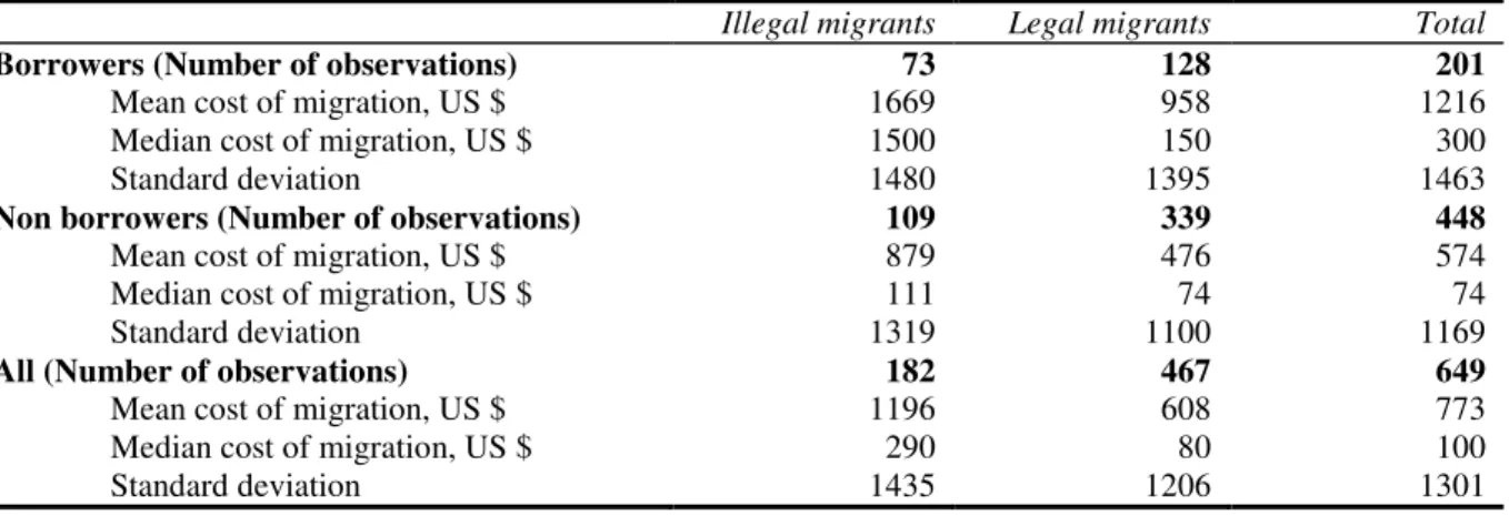
As mentioned in section 2, legal status is part of migration costs. The CBS-AXA 2006 survey offers a direct measure of the migration costs in the dataset: total money spent to cover migration, and whether the migrant needed to borrow money. Unfortunately, these questions were not routinely informed for our sample of 939 migrants. This prompted us to deploy a two-step econometric estimation strategy. In step one, we run regressions on the subsample for which we have duration and legal status data (939 individuals), and in step two, we run estimations on the sub-sample of migrants for whom we also have costs and borrowing data (649 individuals). The statistics presented in Table 2 describe the link between legal status, migration costs, and borrowing needs.
Table 2 Summary statistics on legal status, migration costs, and borrowing needs
Illegal migrants Legal migrants Total
Borrowers (Number of observations) 73 128 201
Mean cost of migration, US $ 1669 958 1216
Median cost of migration, US $ 1500 150 300
Standard deviation 1480 1395 1463
Non borrowers (Number of observations) 109 339 448
Mean cost of migration, US $ 879 476 574
Median cost of migration, US $ 111 74 74
Standard deviation 1319 1100 1169
All (Number of observations) 182 467 649
Mean cost of migration, US $ 1196 608 773
Median cost of migration, US $ 290 80 100
Standard deviation 1435 1206 1301
Two main results emerge from this table. First, illegal migrants face two-fold higher migration costs than legal migrants (nearly 1200 US$ for illegal migrants versus 600 US$ for legal migrants). Second, a larger proportion of irregular migrants need to borrow to finance the trip to the destination country (almost 40% of illegal migrants are borrowers compared to only 27% of legal migrants). The combination of these facts implies that irregular migrants need to repay more for migration than legal migrants.
Table 3 gives the definitions and basic descriptive statistics of the other variables used in the analysis. To test hypothesis 2, we need data on wages in the host and home countries, but unfortunately, the dataset does not contain these variables. However, like Dustmann and Kirchkamp (2001), we do use a number of factors as proxies of the relative productivity of a particular migrant, i.e. gender, age at first migration trip, level of education, problems with host country language, destination, and type of location
11 abroad (rural or urban).5 Level of education before emigration and age at first migration (mean migrant age is 31.65) should be positively related to the migrant’s earnings potential. Conversely, women (38%) and migrants who do not speak the destination-country language (13%) are assumed to have a lower relative wage abroad. We also expect that migrants employed in an EU country (8%) would have a relatively higher wage abroad than a migrant working in a non-EU country. Migrants working in the CIS (36%) are assumed to have the lowest relative wages. Moreover, as documented in Lücke et al. (2007), wages are highly dependent on gender and location abroad. To capture this joint effect, we also introduce an interaction term between gender and destination. Furthermore, migrants working in town or cities (44%) in the destination country are also assumed to have higher earnings abroad. As Lindström (1996) suggests, compared with the agricultural sector, urban labour markets provide migrants with a greater variety of jobs. Three indicators relative to social, infrastructure and economic development (SDI, IDI and EDI) are used to test the potential impact of regional development of the origin community on the duration of migration (hypothesis 3). Since the levels of economic, social and infrastructural development are correlated, we introduce them separately in the regressions. This is achieved by generating dummy variables for each of these indicators, separating “depressed regions” from “developed regions” compared to the two main cities of Moldova.6 We also introduce dummy variables for the geographical zones of Moldova (Center, North and South) to account for other differences between regions. Finally, we use four variables as proxies for family ties (hypothesis 4): proportion of dependents, and the migrant’s position in the family unit (household head, spouse or child). Table 3 Definitions of variables and their descriptive statistics.
Variable Definition Mean SD
Individual Characteristics
Gender 1 if the migrant is a woman, else 0 0.38 0.49
Age Age at first migration trip 31.65 9.75
Primary 1 if the migrant has no or primary education, else 0 0.36 0.48 Tertiary 1 if the migrant has secondary or tertiary education, else 0 0.39 0.49 University 1 if the migrant has university education, else 0 0.19 0.40 Post-university 1 if the migrant has post-university education, else 0 0.05 0.23 Romanian 1 if the migrant has dual Romanian citizenship, else 0 0.03 0.16
Household Characteristics
Dependents Proportion of dependents in the household 0.20 0.20
Hh head 1 if the migrant is the household head, else 0 0.36 0.48 Hh hd’s spouse 1 if the migrant is the household head’s spouse, else 0 0.18 0.38 Hh hd’s child 1 if the migrant is the household head’s child, else 0 0.16 0.36 Hh wealth decline 1 if the household’s subjective perception is that their wealth
deteriorated between 1998 and 2006, else 0
0.35 0.48
Social Capital
Other migrants Number of other migrants in the household 1.95 1.60 Network 1 if the migrant received help from contacts abroad, else 0 0.62 0.49
5
Dustmann and Kirchkamp (2001) use two proxies to account for the relative productivity of a particular migrant: education before emigration and occupational class upon arrival to the host country.
6
12 Destination Country Characteristics
EU 1 if the migrant works in an EU country7, else 0 0.08 0.27
CIS 1 if the migrant works in the CIS8, else 0 0.37 0.48
Other 1 if the migrant works in other countries, else 0 0.55 0.50 Urban destination 1 if the migrant works in an urban location, else 0 0.45 0.50 Home Country: Community and Regional Characteristics
Urban origin 1 if the migrant arrived from an urban location, else 0 0.30 0.46 Locality size 1 if the migrant arrived from a locality with more than 50000
inhabitants, else 0
0.11 0.31 North 1 if the migrant is arrived from the Northern region, else 0 0.28 0.45 Centre 1 if the migrant is arrived from the Central region, else 0 0.46 0.50 South 1 if the migrant is arrived from the Southern region, else 0 0.26 0.44
SDI Social development index (min -1.63 and max 5) 0.63 1.83
IDI Infrastructure development index (min -1.59 and max 1.3) 0.16 0.68
EDI Economic development index (min -1.06 and max 2) 0.28 0.92
Migration experience Migration experience
Illegal exp. 1 if the migrant had illegal migration experience, else 0 0.25 0.44 Illegal entry 1 if the migrant gained illegal entry into the dest. country, else 0 0.21 0.41 Illegal f. job 1 if the migrant had an illegal first job in the dest. country, else 0 0.26 0.44 No language 1 if the migrant did not know the language of the destination
country before migration, else 0
0.13 0.34
Observations Observations 939
Households Households 762
4. Analysis
The duration models used in our analysis assume a baseline hazard function. This function corresponds to the hazard when all covariates are zero. Equation (1) depicts the effect of covariates on this hazard:
h(t)=h0(t)µ with µ=exp(βX) (1)
The intercept term h0 serves to scale the baseline hazard, X is a vector of regression covariates. When x=0, µ=1 and h(t)=h0.
The corresponding survival function, i.e. the cumulated time before failure, is the following:
S(t) = exp[-h0(t)µ] (2)
In order to simplify the interpretation of the effects of the covariates on duration, the survival function (equation 2) is specified in accelerated failure time corresponding to a linear function between the natural logarithm of the survival time and the covariates:
z
x
t
=
β
+
ln
, ort
=
µ
exp(z
)
(3)where t is the survival time and z is the error with density
f
()
. The distributional form of the error term determines the regression model. If we letf
()
be the normal density, the lognormal regression7
EU countries in the CBS-AXA survey include Austria, Belgium, the Czech Republic, France, Germany, Greece, Ireland, Italy, Poland, Portugal, Slovenia, Spain, and the United Kingdom.
8
13 model is obtained. Similarly, if we let
f
()
be the logistic density, the log-logistic regression is obtained. Settingf
()
equal to the extreme-value density yields both the exponential and the Weibull regression models.From the accelerated failure time model, it is possible to calculate time ratios (
j i
t
t
=
)
exp(
β
) which are quite similar to marginal effects and hence very convenient to interpret. 9 This is the presentation of the results we propose in Table 5. In model 1 for example,, the time ratio for the gender dummy equals 1.43. This means that duration of migration is 43% longer for a woman than for a man.Moreover, duration models allow the effect of the time already spent itself to have an effect on survival time. For example, we can think that when a migrant has already spent two years abroad, he/she is more prone to return. The Weibull function in particular allows this possibility. Its baseline hazard is shown through equation (4):
h0(t)=pt p-1
(4) Hence, its hazard function is:
h(t)=ptp-1µ (5)
and hence the corresponding survival is:
S(t)=exp[- ptp-1µ] (6)
In equation (6), when p>1, the time already spent abroad decreases the duration, and when p<1, the time already spent abroad increases the duration. The results of the Weibull model presented at the bottom of Table 5 show that in our sample, time already spent abroad decreases the duration of migration, as the estimated p parameter is greater than one.
Furthermore, we suspected that our sample contained unobserved heterogeneity: as time goes by, most returning individuals will disappear from the dataset, leaving a more homogeneous population comprising only those who are less likely to return home. The way to correct for this kind of heterogeneity is to introduce, at the level of an observation or group of observations, an unobservable multiplicative effect, α, on the hazard function, known as a “frailty effect”, such that:
( | ) { ( )}
S t
α
= S t α (7)9
Quoting Jenkins (2005), note that:
k k X t ∂ ∂ = ln
β with
t
=
µ
exp(z
)
. Therefore, if two persons i and j are identical in all but the kthcharacteristics, i.e. Xim=Xjm for all m∈
{
1,...K}
, and have the same z, thenexp[
k(
ik jk)]
j i
X
X
t
t
−
=
β
. If, in addition, Xik-Xjk=1, i.e. there is a one unit change in Xk ceteris paribus, then
j i
t
t
=
)
exp(
β
.14 where S(t) is the survivor function. Since α is unobservable, we have to suppose that it follows a parametric distribution. Two functions are commonly used: the Gamma and the inverse Gaussian. As reported in Table 4, we estimate the model with all available distributions (Exponential, Weibull, Gompertz, Log-normal, Log-logistic and Cox) and test corrections for heterogeneity using Gamma and inverse Gaussian functions at individual level and household level. The most powerful model, with lower BIC and AIC values, is a Weibull model with a Gamma distribution for unobserved household heterogeneity.
Table 4. Comparison of models for migration duration: Moldovan migrants, 2006
Inverse Gaussian distribution Gamma distribution
AIC BIC AIC BIC
Models with correction for unobserved household heterogeneity
Weibull 1293.985 1376.346 1259.856 1342.218
Exponential 1333.565 1411.082 1328.886 1406.403
Log-logistic 1270.713 1353.075 1268.723 1351.085
Log-normal 1316.46 1398.822 1314.411 1396.773
Gompertz 1315.841 1398.203 1315.626 1397.988
Cox ---a ---a ---a ---a
Models with correction for unobserved individual heterogeneity
Weibull ---a ---a 1289.829 1372.191
Exponential 1341.262 1418.779 1337.943 1415.46
Log-logistic 1286.183 1368.545 1284.534 1366.896
Log-normal 1326.034 1408.396 1325.832 1408.194
Gompertz 1316.186 1398.548 1316.186 1398.548
Cox ---a ---a ---a ---a
Note: a Model unable to achieve convergence
Table 5 contains the results of the duration model estimations. Model 1 contains all potentially influential covariates. Model 2 includes only the significant variables and is used to generate the predictions and conclusions. Models 3 and 4 test for alternative proxies for irregular migration. Model 5 takes into account the potential effect of being an irregular migrant in an EU country. Models 6 to 8 introduce migration costs variables and are therefore estimated on a reduced sample (according to valid available data on migration costs).
15
Table 5. Time ratio estimates for duration regression models using Weibull distribution with Gamma correction for unobserved household heterogeneity.10
Model 1 Model 2 Model 3 Model 4 Model 5 Model 6 Model 7 Model 8
Time Ratio (t) Time Ratio (t) Time Ratio (t) Time Ratio (t) Time Ratio (t) Time Ratio (t) Time Ratio (t) Time Ratio (t)
Individual Characteristics Gender 1.43** 1.34** 1.31** 1.28* 1.37** 1.42** 1.35* 1.37** (2.35) (2.20) (2.07) (1.90) (2.37) (2.24) (1.92) (1.99) Age 1.03 (0.91) Age squared 1.00 (-1.42) Tertiary 1.10 (0.83) University 1.06 (0.38) Post-university 1.26 (0.94) Romanian 2.79** 2.58** 2.49** 2.41* 2.61** 2.30* 2.26* 2.15* (2.21) (2.02) (1.99) (1.90) (2.02) (1.79) (1.81) (1.71) Household Characteristics Dependents 0.44*** 0.55** 0.56** 0.54*** 0.53*** 0.63* 0.74 0.76 (-3.06) (-2.46) (-2.49) (-2.68) (-2.64) (-1.71) (-1.14) (-1.05) Hh head 0.05*** 0.04*** 0.04*** 0.05*** 0.04*** 0.06*** 0.08*** 0.08*** (-11.54) (-12.90) (-13.23) (-12.58) (-12.98) (-10.46) (-7.95) (-7.69) Hh hd’s spouse 0.05*** 0.05*** 0.05*** 0.06*** 0.05*** 0.07*** 0.08*** 0.09*** (-13.25) (-13.70) (-13.91) (-13.05) (-13.71) (-10.59) (-8.47) (-8.16) Hh hd’s child 0.06*** 0.06*** 0.06*** 0.07*** 0.06*** 0.09*** 0.11*** 0.12*** (-12.74) (-12.71) (-12.93) (-12.13) (-12.73) (-9.25) (-7.33) (-6.92) Hh wealth decline 1.31** 1.35*** 1.37*** 1.38*** 1.33** 1.76*** 1.65*** 1.67*** (2.33) (2.64) (2.79) (2.87) (2.46) (4.33) (3.85) (3.93) Social capital Other migrants 1.07 (1.25) Network 1.05 10 j i
T
T
=
β
16
Model 1 Model 2 Model 3 Model 4 Model 5 Model 6 Model 7 Model 8
Time Ratio (t) Time Ratio (t) Time Ratio (t) Time Ratio (t) Time Ratio (t) Time Ratio (t) Time Ratio (t) Time Ratio (t)
(0.43)
Destination Country Characteristics
EU 1.93** 1.88*** 1.94*** 1.97*** 1.48 2.49*** 1.69* 1.75** (2.02) (2.64) (2.80) (2.88) (1.44) (3.55) (1.94) (2.06) CIS 0.96 0.90 0.89 0.95 0.93 0.53*** 0.58** 0.56** (-0.16) (-0.61) (-0.70) (-0.28) (-0.40) (-2.72) (-2.35) (-2.49) Urban destination 0.88 (-0.57)
Home Country: Community and Regional Characteristics
Urban origin 1.23 (1.48) Locality size 1.37 (1.27) Centre 0.94 (-0.45) South 0.83 0.79* 0.78** 0.83 0.80* 0.80* 0.82 0.80* (-1.30) (-1.86) (-1.99) (-1.60) (-1.76) (-1.71) (-1.59) (-1.74) Socially depressed regions 1.31* 1.20 1.21* 1.24** 1.21* 1.09 1.10 1.08 (1.68) (1.64) (1.76) (2.03) (1.75) (0.75) (0.85) (0.67) Socially developed regions 0.91 (-0.59) Migration experience Illegal exp. 1.37** 1.37** 1.26* 1.29* 1.19 1.17 (2.35) (2.40) (1.66) (1.88) (1.26) (1.16) Illegal entry 1.31** (2.01) Illegal f. job 1.03 (0.25) No language 1.42* 1.43* 1.46** 1.65*** 1.47** 1.23 1.11 1.11 (1.87) (1.90) (2.11) (2.81) (2.06) (1.11) (0.53) (0.56) EU*Gender 0.74 (-0.80) CIS*Gender 0.58** 0.64** 0.66* 0.67** 0.61** 0.53*** 0.58** 0.56** (-2.33) (-2.11) (-1.95) (-1.97) (-2.29) (-2.72) (-2.35) (-2.49)
17
Model 1 Model 2 Model 3 Model 4 Model 5 Model 6 Model 7 Model 8
Time Ratio (t) Time Ratio (t) Time Ratio (t) Time Ratio (t) Time Ratio (t) Time Ratio (t) Time Ratio (t) Time Ratio (t)
Illeg.status x UE 2.12* (1.78) Costs of migration 1.00*** 1.00** (4.19) (2.49) Borrower 0.86 0.76** (-1.34) (-2.02) Costs x borrower 1.00* (1.69) Constant 93.90*** 153.80*** 151.74*** 130.34*** 151.70*** 98.67*** 72.90*** 71.70*** (7.37) (20.27) (20.89) (19.27) (20.34) (15.93) (11.74) (11.29) Number of obs. 935 939 955 937 939 649 649 649 Number of households 759 762 771 757 762 547 547 547 Number of failures 267 267 273 275 267 210 210 210 (%) (28.43) (28.43) (28.59) (29.35) (28.43) (32.36) (32.36) (32.36) P 1.91*** 1.94*** 1.98*** 2.04*** 1.97*** 1.93*** 2.00*** 2.02*** (8.47) (8.67) (9.36) (9.16) (8.75) (7.56) (6.95) (6.88) Theta 1.99*** 2.29*** 2.36*** 2.49*** 2.34*** 1.65** 1.70* 1.75* (3.24) (4.14) (4.63) (4.66) (4.29) (1.99) (1.75) (1.82) chi² 235.04*** 212.66*** 222.19*** 209.51*** 215.89*** 146.41*** 167.43*** 170.39*** AIC 1262.55 1259.86 1277.07 1270.96 1258.63 931.43 914.40 913.44 BIC 1407.77 1342.22 1359.72 1353.29 1345.84 1007.51 999.44 1002.95
18 The estimated p value shows a negative dependency of duration of stay with time already spent abroad.11 Figure 2 shows that it is extremely unlikely a typical Moldovan will spend more than six years in the host country.
Figure 2. Weibull survival regression with Gamma household heterogeneity
Reference migrant Legal migrant Illegal migrant
In Figure 2, the solid line (derived by centering all of the continuous and dummy covariates on their respective means) represents the length of migration experienced by a typical migrant. The survival decreases rapidly over the first three years before flattening out abruptly at around the four-years mark to reach roughly zero thereafter. The predicted model thus concludes that a very small proportion of Moldovan migrants should stay abroad after four years of migration, even if the maximal observed duration in our sample is 15 years.
In Figure 2, the dashed line above the survival plot for a typical migrant is the estimated survival for illegal migrants. The graph highlights how illegal status in the foreign country increases the duration of the optimal stay.
11
For a definition of p see above, equations (4), (5) and (6).
0 .2 .4 .6 .8 1 0 2 4 6 8 10
19 Table 6. Predicted mean and median durations at covariate sample means for return/censored and legal/illegal migrants
All All Return
migrants
Censored migrants
Nb. Obs. 939 267 672
Predicted mean duration (months) 60.46 13.70 79.04
Predicted median duration(months) 57.12 12.94 74.68
Legal migrants
Nb. Obs. 700 208 492
Predicted mean duration (months) 52.84 12.97 69.70
Predicted median duration (months) 49.92 12.25 65.85 Illegal migrants
Nb. Obs. 239 59 180
Predicted mean duration (months) 82.78 16.28 104.58
Predicted median duration (months) 78.21 15.39 98.81
An interesting outcome of the duration models is the prediction of potential length of migration for censored observations (72% of migrants in model 2). According to Table 1, the uncompleted mean migration duration is 25 months (i.e. just over 2 years). Model 2 predicts that the real duration for this subpopulation should be about 5 years. The contrast is equally striking between illegal and legal migrants. While documented migrants have a predicted mean duration of nearly 4½ years, illegal migrants are likely to spend nearly seven years abroad. If illegal status is a proxy for more expensive migration costs, lower earnings or lower net benefits of migration, then it can explain this result. We test this hypothesis in the second part of the econometric analysis (Models 6 to 8 of Table 5). We now turn to the interpretation of the results on the whole sample.
Model 1 rejects the influence of some potential factors. Individual characteristics such as age at first migration and education level do not have an effect on time spent abroad. Similarly, established networks have no effect on length of migration stay. Looking at destination country-focused characteristics, CIS and urban areas do not attract migrants for longer durations than other areas. Concluding on non-significant variables, migrants from the centre of Moldova and from urban regions do not seem to show singular patterns of migration behaviour. On the other hand, most of the foreseeable factors do have an influence on time spent abroad.
Model 2 contains only significant covariates and includes a dummy variable accounting for illegal migration experience in the destination country (hypothesis 1). Model 3 contains a dummy for illegal entry into the destination country and Model 4 considers the impact of a first illegal job on duration of stay. Each of these potential indicators of illegality increases the time spent abroad.12 The most significant indicator of illegality is the dummy for illegal experience. We therefore choose to keep this variable for the remainder of the analysis. Model 2 is therefore our reference estimation. It shows that migration duration is 1.37 times higher for an illegal migrant than their legal counterpart. This result is consistent with Magris and Russo’s (2009) and Reichert and Massey’s (1984) conclusions, but runs counter to Pinger’s (2010) and Lindström’s (1996) findings. Pinger’s (2010)
12 A candidate fourth indicator could have been lack of a residence permit. We opted to ignore this variable as we suspected potential
endogeneity with duration of migration: most of the destination countries require people to have been living in the country for a given period before they can apply for a residence permit.
20 empirical study on the determinants of temporary and permanent migration uses the same “CBS-AXA 2006” dataset as used in this paper. However, Pinger uses a standard probit model to compare permanent versus temporary migration. Our work, which is based on duration of migration and which uses a parametric estimation, diverges from Pinger to demonstrate that being undocumented increases time spent abroad. The potential lower wage and/or higher migration costs for illegal migrants can partly explain this result. As irregularity can have a higher effect in the EU countries, we introduce an interaction variable combining illegality and EU dummy in Model 5. The results show that the migration duration for irregular migrants is even longer when they go to EU countries.
Extending the investigation into the link between undocumented migrants and migration expenditures, Models 7 and 8 show the results after introducing migration costs and borrowing needs into the initial regression. Migration costs are highly significant and, as expected, the effect of legal status vanishes when costs are introduced into the model. Of course, to be sure that this result is not due to the reduced size of the sample, we re-ran the initial model without the costs on the sub-sample for which we have migration expenditure data (Model 6). The time ratio of the indicator on illegal experience (1.29) is close to that obtained on the whole sample (1.37) and is significant at a 10% risk rather than at a 5% risk. Therefore, the disappearance of the illegal status effect in Model 7 is not attributable to the reduction of sample size but to the fact that migration costs were introduced into the regression. The last test we run is to infer whether there are differences in the impact of migration expenditures between borrowers and non-borrowers. Model 8 thus includes an interaction covariate between migrant costs and migrant borrowers. The results show a slightly larger impact of migration costs for borrowers, but higher migration costs still drive longer duration of stay for non-borrowers.13 Hence, illegal migrants come back to Moldova later than legal migrants, in part because they face higher migration costs.14
From a purely statistical standpoint, Görlich and Trebesch (2008) also observed that undocumented migrants tend to concentrate in the seasonal-migrant sample. We ran regressions including a dummy variable for seasonal migrants. This factor proved significant and exerted a negative influence on duration without changing any of the other results. As we suspected this factor showed potential endogeneity since the questionnaire defined a seasonal migrant as any person having spent less than 3 consecutive months abroad, we removed it from the model. We also ran the model on the subsample of non-seasonal migrants. The main results were not different from the principal model, and only certain control variables were no longer significant.15
Concerning the effect of factors used as proxies for wages differentials (hypothesis 2), we find that women stay longer abroad. In order to further explore the gender dimension, we introduce an
13
The precise values of the coefficients for costs are 1.000318 in Model 7 and 1.00224 in Model 8. The precise value of the coefficient for costs x borrower in Model 8 is 1.000225.
14
Illegal status could also be perceived as a proxy for lower expected wage abroad. Nevertheless, as documented further on, we introduce a number of other variables that can influence potential earnings in order to clear legal status for this likely influence.
21 interaction term between destinations and gender. Women going to CIS countries come back sooner, whereas there is no particular effect for women going to EU. Migrants who do not know the destination country’s language stay longer. If gender (in particular women in CIS) and mastery of the foreign language were negatively correlated to expected wage, then these results would conclude in favour of the target income theory.
Next, we analyze the push and pull factors of the migrant’s region of origin (hypothesis 3). The dataset offers three potential indicators of regional development, i.e. economic, infrastructural and social indexes. We introduced these indicators separately into Model 1 (results not shown). Only the dummy variable for socially-depressed regions was significant and subsequently kept in the analysis. The results show that Moldovan migrants from socially-depressed regions spend more time abroad. Echoing Lindström (1996) and Reyes (2001), we find that a region with better social development acts as a pull factor and prompts migrants to come back sooner if they can expect a better way of life in their home region.
Finally, we examine the influence of family ties on duration of stay (hypothesis 4). In contrast with Görlisch and Trebesch (2008), we find very strong effects of household composition on the migrant’s duration of stay. The household head, their spouse or their child spend dramatically less time abroad. For example, a household head migrant or their spouse would stay only one month in the destination country where a typical migrant sharing otherwise identical characteristics is expected to spend two years in the same place. Similarly, an increasing proportion of dependent members in the family decreases the migrant’s duration of stay. Focusing on the influence of the family’s economic situation, Model 2 shows that belonging to a household that has experienced a decline in its perceived level of income between 1998, i.e. immediately after the Russian financial crisis, and the 2006 survey increases the migrant’s duration of stay. This is almost certainly due to the dependency of this type of family on remittances.
5. Conclusion
This paper investigates the factors driving migrant decisions on migration duration abroad. We focus on the effect of the migrant’s legal status. We run a duration model using a Moldovan micro-survey carried out in 2006 and complemented with regional development data from Roscovan and Galer (2006). The estimations show that irregular migrants spend significantly longer periods abroad. Further investigation demonstrates that this effect is driven by significantly higher migration costs. From a policy perspective, our findings on irregular migration may well be highly relevant, as they question the outcome of restrictive migration policies. Our findings suggest that extending effective duration of stay compared to optimal migration duration reduces the potential circularity of migration episodes. The net result is that restrictive migration policies generate stocks of unmotivated illegal migrants in the host countries, which is ultimately the reverse effect of the stated policy goals. This
22 paper, like an increasing number of migration literature papers converging on the same conclusions (Constant and Zimmermann (2011) and Magris and Russo (2009) are good examples) contributes to further arguments for redefining migration policy.
The estimated duration model goes on to highlight certain characteristic features of migrant choices. First, the more time the migrant has already spent abroad, the more prone he/she is to come back. Migrants presenting an unfinished migration duration spell at the time of the survey post a mean stay abroad of two years and seven months. According to our results, they are likely to return home after five more years abroad. Family composition exerts a strong pull effect on the migrant: the duration of stay of a household head is just 4% that of a typical migrant. The same scale of effect holds true for the household head’s spouse or child, as well as for the proportion of dependents in the family. However, we did not find any influence of networks on duration decisions. This refutes the findings of other studies on Moldovan migrants, including Görlich and Trebesch (2008), who, conversely to our study, found no evidence of influence of family ties yet a significant impact of networks.
We introduce a number of proxy variables capable of influencing the wage differential between home and host country. Only gender increases time spent abroad, while neither age at first migration nor education exert any influence on duration of stay. Migration duration is 30% longer for women than men, except for women migrating out to the former Russian Republics, where migration duration will be 40% shorter than for men migrating to the same destination). These differences are explained by the fact that women hold different types of jobs to men in different destinations. Certain regional characteristics of the origin country play a significant role in the migrant’s decision. Moldovan emigrants from poorer regions, like Mexican emigrants –as documented by Linström (1996) – spend shorter spells abroad. These results may be due to the fact that income target and investment opportunities are lower for migrants from less-developed regions of the origin country.
Acknowledgments: We would like to thank Giuseppe Russo, the participants of the CERDI internal seminar,
and the anonymous referees for very helpful comments and suggestions.
References
AMM-ILO (2004) Nota Informativa privind Studiul - Migratia de munca si remitentele in R. Moldova. Alianta Microfinantare Moldova, Chisinau
Avato J (2009) Migration pressures and immigration policies: new evidence on the selection of migrants. Social Protection Discussion Papers 52449, The World Bank
Bauer TK, Gang IN (1998) Temporary Migrants from Egypt: How long do they stay abroad? Working Paper 3, IZA, Bonn
Berg EJ (1961) Backward-sloping labor supply functions in dual economies: the African case. Quarterly Journal of Economics, 75:468-492
Bijwaard GE, (2010) Immigrant migration dynamics model for The Netherlands. J Popul Econ 23:1213–1247
Borodak D, Piracha M (2011) Occupational Choice of Return Migrants in Moldova. Eastern European Economics, 49(4):23–43.
23 Cassarino J-P (2004) Theorising return migration: the conceptual approach to return migrants
revisited. International Journal on Multicultural Societies 6(2):253-279
Carrión-Flores CE (2006) What Makes You Go Back Home? Determinants of the duration of migration of Mexican immigrants in the United States. Society of Labor Economists Annual Meeting, Cambridge MA, May 5-6, 2006
CBS-AXA Consultancy (2005) Migration and Remittances in Moldova, 2005. International Organization for Migration, Chisinau
Constant A, Zimmermann KF (2011), Circular Migration and Repeat Migration: Counts of Exits and Years Away from the Host Country. Population Research and Policy Review 30:495-515 Constant A, Zimmermann KF (2003) The dynamics of repeat migration: a Markov chain analysis.
Discussion Paper 885, IZA, Bonn
Coulon A, Piracha M (2005) Self-selection and the performance of return migrants: the source country perspective. J Popul Econ 18(4):779-807
Cuc M, Lundback E, Angelovska-Bezoska A, Ruggiero E, Bouton L, Sandu M (2005) Republic of Moldova: Selected Issues. Country Report no. 05/54, International Monetary Fond
Departamentul statisticii al Republicii Moldova (2004) Statistical Yearbook of Moldova 2003. Departamentul statisticii al Republicii Moldova, Chisinau
Detang-Dessendre C, Molho I (1999) Migration and changing employment status: A hazard function analysis. Journal of Regional Science 39:105-123
Djajic S, Milbourne R (1988) A general equilibrium model of guest-worker migration: a source-country perspective. Journal of International Economics 25:335–351
Dustmann C, Kirckkamp O (2002) The optimal migration duration and activity choice after re-migration. Journal of Development Economics 67:351-372
Dustmann C (2003) Return migration, wage differentials and the optimal migration duration. European Economic Review 47(2): 353–69
European Commission (2005) Migration and Development: Some Concrete Orientations. European Commission 390, Brussels
Fidrmuc J (2004) Migration and regional adjustment to asymmetric shocks in transition economies. Journal of Comparative Economics 32:230–247
Galer L (2004) Discrepanţe teritoriale în dezvoltarea economico-socială a Republicii Moldova. Moldova Habitat 46, Chisinau
Ghencea B, Gudumac I (2004) Labour Migration and Remittances in the Republic of Moldova. Moldovan Microfinance Alliance Report, Chisinau
Goerlich D, Trebesch C (2008) Mass migration and seasonality evidence on Moldova’s labour exodus. Review of World Economics 144(1):107-133
Hagen-Zanker J, Siegel M (2007) The determinants of remittances: A comparison between Albania and Moldova. Working paper 2009-007, Maastricht Graduate School of Governance
Harris J, Todaro M (1970) Migration, unemployment and development: a two-sector analysis. American Economic Review 60:126-142
Hill JK (1987) Immigrant decisions concerning duration of stay and migratory frequency. Journal of Development Economics, 25:221–234
IOM (2004) Return Migration: Policies and Practice in Europe. International Organization for Migration and the Advisory Committee on Aliens Affairs, The Netherlands
Lindstrom DP (1996) Economic opportunity in Mexico and return migration from the United States. Demography 33(3):357–374
Lindstrom DP, Lauster N (2001) Local economic opportunity and the competing risks of internal and US migration in Zacatecas, Mexico. International Migration Review 35(4):1232-1256
Longva P (2001) Out–migration of immigrants: implications for assimilation analysis. Memorandum 04/2001, University of Oslo
Lücke M, Mahmoud TO, Pinger P (2007) Patterns and trends of migration and remittances in Moldova. International Organization for Migration, Chisinau. (http://www.iom.md)
Magris F, Russo G (2009) Selective immigration policies, human capital accumulation and migration duration in infinite horizon. Research in Economics 63(2):114-126
Magris F, Russo G (2001) Frontiers Openness and the Optimal Migration Duration. DELTA Working Papers 12, ENS, Paris
24 Massey D (1990) Social structure, household strategy, and the cumulative causation of migration.
Population Index 56:3–26
Massey D, Lian Z (1989) The long-term consequences of a temporary worker program: The US Bracero experience. Population Research and Policy Review 8:199–226
Mosneaga V (2007) The Labor Migration of Moldovan Population: Trends and Effects. Working Paper 3, SOCIUS, Lisboa
Orozco M (2008) Looking rorward and including migration in development: remittance leveraging opportunities for Moldova. International Organization for Migration, Chisinau
Palloni A, Massey D, Ceballos M, Espinosa K, Spittel M (2001) Social Capital and International Migration: A test using Information on Family Networks. American Journal of Sociology, 106(5):1262-1298
Parsons CR, Skeldon R, Walmsley TL, Winters LA (2007) Quantifying International Migration: A Database of Bilateral Migrant Stocks. Policy Research Working Paper 4165, The World Bank. Pinger P (2010) Come Back or Stay? Spend Here or There? International Migration 48: 142-173 Pyshkina TV (2002) Economic Consequences of the Migration of Labour from the Republic of
Moldova. WIDER Conference on Poverty, International Migration and Asylum, 27–28 September 2002, Helsinki
Roşcovan M, Galer L (2006) Raitingul de dezvoltare a unităţilor administrativ-teritoriale ale Republicii Moldova. Moldova Urbană 1, Chisinau
Reyes BI (2001) Immigrant trip duration: The case of immigrants from Western Mexico. International Migration Review 35(4):1185-1204
Reyes BI (2004) Changes in trip duration for Mexican immigrants to the United States. Population Research and Policy Review 23:235–257
Reichert J, Massey D (1984) Patterns of U.S. Migration from a Mexican Town. In: Patterns of Undocumented Migration: Mexico and the United States, edited by R. Jones, Totowa, NJ: Rowman and Allanheld, 93-109
Rivera-Batiz FL (1999) Undocumented workers in the labor market: an analysis of the earnings of legal and illegal Mexican immigrants in the United States. J Popul Econ 12(1):91–116
Sjaastad LA (1962) The costs and returns of human migration. Journal of Political Economy, Supplement 70:80-93
Stark O, Helmenstein C, Yegorov Y (1997) Migrants’ savings, purchasing power parity, and the optimal duration of migration. International Tax and Public Finance 4:307–324
SOPEMI – OECD (2008) International Migration Outlook. Organisation for Economic Co-operation and Development, Paris
Todaro MP (1969) A model of labor migration and urban unemployment in less developed countries. The American Economic Review 59:138-148
van Dalen HP, Groenewold G, Schoorl JJ (2005) Out of Africa: What Drives the Pressure to Emigrate? J Popul Econ 18(4):741-778
Zahniser SS (1999) Mexican Migration to the United States: The Role of Migration Networks and Human Capital Accumulation. Garland Publishing, New York
25 Separate appendix to the paper
Table 1a. Selected sample characteristics
Entire sample (active population)
Non-migrants
sample difference Migrants sample
Migrants without available duration information difference Migrants with available duration information N 10555 6.833 3722 2.787 935 Gender 0.53 0.53 0.01 0.52 0.51 0.13*** 0.38 Primary 0.36 0.37 0.01 0.36 0.30 -0.06** 0.36 Tertiary 0.31 0.29 -0.05*** 0.34 0.34 -0.05* 0.39 University 0.21 0.21 -0.01 0.22 0.26 0.07** 0.19 Post-university 0.11 0.13 0.05*** 0.08 0.10 0.05*** 0.05 Romanian 0.04 0.04 0.00 0.04 0.04 0.01 0.03 Dependents 0.16 0.15 -0.03*** 0.18 0.16 -0.03** 0.20 Hh head 0.29 0.35 0.16*** 0.19 0.11 -0.25*** 0.36 Hh hd’s spouse 0.29 0.32 0.07*** 0.25 0.12 -0.06** 0.18 Hh hd’s child 0.18 0.18 -0.01 0.19 0.14 -0.02 0.16 Hh wealth decline 0.31 0.29 -0.06*** 0.35 0.28 -0.07** 0.35 Other migrants 0.89 0.15 -2.10*** 2.24 1.57 -0.37*** 1.94 Network 0.11 0.01 -0.31*** 0.32 0.57 -0.04 0.62 Urban origin 0.36 0.39 0.08*** 0.31 0.32 0.02 0.30 Locality size 0.20 0.24 0.11*** 0.13 0.15 0.04* 0.11 North 0.27 0.26 -0.03** 0.29 0.29 0.01 0.28 Centre 0.53 0.55 0.07*** 0.48 0.44 -0.02 0.46 South 0.20 0.19 -0.04*** 0.23 0.27 0.01 0.26 ecoq1 0.21 0.19 -0.06*** 0.25 0.24 -0.03 0.27 ecoq2 0.22 0.21 -0.03** 0.24 0.23 0.01 0.22 ecoq3 0.26 0.26 -0.01 0.27 0.27 0.01 0.27 ecoq4 0.31 0.34 0.10*** 0.24 0.26 0.02 0.24 socioq1 0.22 0.20 -0.03** 0.23 0.21 -0.03 0.24
26 socioq2 0.26 0.25 -0.04*** 0.29 0.30 0.01 0.29 socioq3 0.16 0.16 -0.03*** 0.18 0.20 0.01 0.19 socioq4 0.36 0.40 0.10*** 0.30 0.30 0.02 0.28 infraq1 0.21 0.19 -0.04*** 0.23 0.23 0.00 0.23 infraq2 0.25 0.25 -0.01 0.26 0.25 -0.02 0.27 infraq3 0.18 0.16 -0.07*** 0.23 0.22 -0.03 0.25 infraq4 0.36 0.40 0.12*** 0.28 0.30 0.04* 0.26
Age at first migration 31.64 -0.01 31.65
EU 0.08 -0.00 0.08 CIS 0.14 -0.23*** 0.37 Other 0.79 0.23*** 0.56 Urban destination 0.32 0.02 0.30 Illegal exp. 0.25 -0.00 0.25 Illegal entry 0.21 0.00 0.21
Illegal first job 0.27 0.02 0.26
27 Details on regional development data
The dataset on regional development in Moldova used in this paper comes from Roscovan and Galer (2006), who constructed three summary indicators: the economic, social and infrastructure development indexes. The social development index (SDI) combines measures of: 1) number of physicians per 10000 inhabitants, 2) number of hospital beds per 10000 inhabitants; 3) number of infant deaths per 1000 live births; 4) number of students per teacher. The infrastructure development index (IDI) includes: 1) number of cars in private ownership per 1000 inhabitants; 2) dwelling stock per inhabitant; 3) public passenger transportation; 4) number of telephones per 100 inhabitants; 5) length of public roads per inhabitant; 6) length of water piping per inhabitant; 7) length of sewerage system per inhabitant. The economic development index (EDI), which we use to test hypothesis 2b, encompasses: 1) average nominal monthly salary per employee; 2) volume of industrial and agricultural production per inhabitant; 3) volume of services per inhabitant; 4) number of SMEs per inhabitant; 5) rate of urbanization.
All three indexes are normalized. The zero value of each index corresponds to the average national level of development. A positive (negative) value for each index corresponds to a region with higher (lower) level of development than the national average. The economic indicator ranges from -1.06 to 2, the social development index from -1.62 to 5, and the infrastructure development index from -1.59 to 1.3. For all three indicators, the highest possible value indicates the maximum development level (reference level), corresponding to the Chisinau (capital of Moldova) region and the Balti region. These indexes are correlated: coefficients of correlation are 69% between EDI and SDI, 77% between EDI and IDI, and 63% between SDI and IDI.
Table 2a: Distribution of the Moldovan administrative-territorial units stratified by level of development for each summary indicator, 2004.
Indexes Mean SD Min Max Nbr of obs.
Economic development index 0.06 0.78 -1.06 2.0 35
Social development index 0.26 1.34 -1.63 5.0 35
Infrastructure development index 0.04 0.67 -1.59 1.3 35
Source: Roscovan and Galer (2006).
For the econometric analysis, we classified the 35 administrative-territorial units according to level of development. A region is considered as depressed if it scores below zero on one of the corresponding indexes (zero being the average national level). It is considered as developed if the index is higher than zero and different from the reference level, corresponding to the two principal city regions of Moldova. We hence generate three dummies for each index according to this classification.
Table 3a. Distribution of regional development indexes in the regression sample on duration of migration (939 individuals)
Economic development index Social development index Infrastructure development index
Level of development Freq.% Freq.% Freq.%
developed regions 27 19 25
depressed regions 49 53 49
reference region 24 28 26