Beam implementation in a nonorthogonal coordinate system: Application to the scattering from random rough surfaces

HAL Id: hal-00256005

https://hal.archives-ouvertes.fr/hal-00256005

Submitted on 22 Apr 2021

HAL is a multi-disciplinary open access

archive for the deposit and dissemination of

sci-entific research documents, whether they are

pub-lished or not. The documents may come from

teaching and research institutions in France or

abroad, or from public or private research centers.

L’archive ouverte pluridisciplinaire HAL, est

destinée au dépôt et à la diffusion de documents

scientifiques de niveau recherche, publiés ou non,

émanant des établissements d’enseignement et de

recherche français ou étrangers, des laboratoires

publics ou privés.

Distributed under a Creative Commons Attribution| 4.0 International License

Beam implementation in a nonorthogonal coordinate

system: Application to the scattering from random

rough surfaces

K. Edee, B. Guizal, G. Granet, A. Moreau

To cite this version:

K. Edee, B. Guizal, G. Granet, A. Moreau. Beam implementation in a nonorthogonal coordinate

system: Application to the scattering from random rough surfaces. Journal of the Optical Society of

America. A Optics, Image Science, and Vision, Optical Society of America, 2008, 25 (3), pp.796-804.

�10.1364/JOSAA.25.000796�. �hal-00256005�

Beam implementation in a nonorthogonal

coordinate system: Application to the scattering

from random rough surfaces

K. Edee,1B. Guizal,2,*G. Granet,1and A. Moreau1 1

Laboratoire des Sciences et Matériaux pour l’Electronique et d’Automatique, CNRS/UMR 6602, Université Blaise Pascal, Les Cézeaux, 63177 Aubière Cedex, France

2

Département d’Optique P.M. Duffieux, Institut Franche-Comté Electronique, Mécanique, Thermique et Optique-Sciences et Technologies, UMR 6174 du CNRS Université de Franche-Comté,

16 Route de Gray 25030 Besançon Cedex, France *Corresponding author: bguizal@univ-fcomte.fr

The C method is known to be one of the most efficient and versatile tools established for modeling diffraction gratings. Its main advantage is the use of a coordinate system in which the boundary conditions apply natu-rally and are, ipso facto, greatly simplified. In the context of scattering from random rough surfaces, we pro-pose an extension of this method in order to treat the problem of diffraction of an arbitrary incident beam from a perfectly conducting (PEC) rough surface. For that, we were led to revisit some numerical aspects that sim-plify the implementation and improve the resulting codes.

1. INTRODUCTION

Actual surfaces are necessarily rough, and the main diffi-culty encountered in the modeling of their interaction with electromagnetic waves is related to their level of roughness. This latter is dependent on the geometry and the wavelength of the incident radiation (i.e., how the sur-face is seen by the wave). Two approximate methods have been developed to study rough surfaces with weak rough-ness and led to analytic expressions of the diffracted in-tensity in terms of the statistical parameters of the sur-faces such as the rms ␴ and correlation length lc. Among

these methods, the most known is the perturbation theory applied to the integral equation of the field [1]. Other ap-proaches use rather heuristic hypotheses concerning the diffraction phenomenon. This is the case for the Kirchhoff approximation [1–3], which can be applied to either shal-low surfaces or surfaces with shal-low radii of curvature. In the so-called resonant domain where the geometrical fea-tures of the scattering surface are of the order of magni-tude of the wavelength, rigorous solutions of the diffrac-tion problem are necessary. This is why exact formalisms have been developed, and one can roughly divide them in two main categories: integral methods [4–7] and differen-tial methods [8]. Integral methods are based on the Green theorem that is used to derive an integral equation that is rigorously solved. As for the differential methods, they rely on solving the partial differential equations directly deduced from Maxwell’s equations and transposed into Fourier space. This is the case for Fourier methods, among which one can find the differential method [8], the Fourier modal method [9], and finally the C method [10,11], which will be used in this work. This approach has been introduced, originally, for the study of

corru-gated waveguides and diffraction gratings. Recently, it has been successfully extended to diffraction of plane waves from nonperiodic surfaces [12–15].

In the present paper we focus, for the sake of concise-ness, on the case of a Gaussian rough surface with Gauss-ian spectrum made of a perfectly conducting (PEC) mate-rial and illuminated by a limited beam. This is by no means a limitation of our approach; the case of dielectric or metallic surfaces can be obtained mechanically from the present work. We will use an improved version of the C method to treat this problem. The article is organized as follows. In Section 2, we outline the main steps of the C method as applied to this problem, and in Section 3, we will specify some properties concerning the eigensolutions that will be exploited in Section 4 in the construction of the incident and diffracted beams. Finally, the method is tested numerically against usual criteria of energy con-servation and our computations are compared to results taken from the literature and based on both integral methods [15] and differential methods [8].

2. STATEMENT OF THE PROBLEM AND

INTRODUCTION TO THE C METHOD

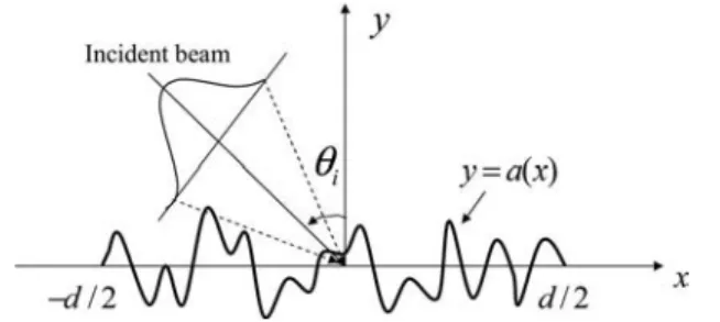
We consider (Fig.1) a rough PEC surface S whose shape is described by a function y = a共x兲 in the orthonormal co-ordinate system共O,x,y,z兲. This surface is invariant along the z direction and is illuminated by an incident wave that can be either TE (the only non-null components of the fields are Ez, Hx, and Hy) or TM (the only non-null

components of the fields are Hz, Ex, and Ey) polarized

such that we are in the case of the so-called classical in-cidence [16]. It is well known that in these cases of

polar-ization, all the field components can be expressed in terms of Ezin the TE case or in terms of Hzin the TM

case. Let us add that throughout this paper, time depen-dence of the fields will be held by the term exp共i␻t兲, where ␻ denotes the circular frequency of the monochromatic in-cident radiation.

The starting point of the C method is the choice of a co-ordinate system in which the diffracting surface (S) coin-cides exactly with a coordinate surface. This has the big advantage of greatly simplifying the process of writing the boundary conditions. The simplest coordinate system is the so-called translation coordinate system (TCS), which is given by

x = u, y = v + a共u兲, z = w. 共1兲 Thus the boundary conditions can be written in a simple way at the coordinate v = 0. In this new coordinate system, it can be shown [13] that ⌿ satisfies the following set of partial differential equations that is valid in the two cases of polarization:

冉

⳵_u⳵_u+ k2_{I 0}

0 I

冊冉

⌿ ⳵_v⌿

冊

=

冉

⳵_{ua˙ + a˙⳵u −}共1 + a˙a˙兲 I 0

冊

⳵v

冉

⌿ ⳵_v⌿

冊

,

共2a兲 where ⌿ = Ezin the TE case and ⌿ = ZHzin the TM case,

with Z denoting the impedance of vacuum. I is the iden-tity operator, k is the wave vector, ⳵u= ⳵ / ⳵u , ⳵v= ⳵ / ⳵v , and

a˙ = da / du .

The second step consists in seeking plane-wave solu-tions under the form

⌿共u,v兲 = exp共− ikrv兲␺共u兲, ⳵v⌿共u,v兲 = exp共− ikrv兲␺r共u兲.

Since ⳵v⬅−ikr, Eq.(2a)can be recast to

冉

⳵_u⳵_u+ k2_{I 0}

0 I

冊冉

␺ ␺r

冊

= − ikr

冉

⳵_{ua˙ + a˙⳵u −}共1 + a˙a˙兲

I 0

冊

冉

␺ ␺r

冊

. 共2b兲 From these equations, it is worth noticing that the profile function comes into play through its derivative a˙, which must exist. However, profiles with rather sharp edges can be treated efficiently by approximating them by smoother ones or by choosing another coordinate system. These is-sues have been addressed in previous works and the in-terested reader can refer to [17–19].

Equation(2b) is then transposed into the spectral do-main by Fourier transformation

fˆ共␣兲 =

冕

−⬁ +⬁

f共u兲exp共− ik␣u兲du, 共3兲 where f共u兲 stands for a˙共u兲, ␺共u兲, or ␺r共u兲. We assume that

the spectrum of the function f共u兲 is a bounded stand. This hypothesis can be justified by the limited spatial exten-sion of the incident beam. Under these conditions, Eq.

(2b)becomes

L1共␣兲 * ⌫ˆ共␣兲 = − ikrL2共␣兲 * ⌫ˆ共␣兲, 共4兲

where L1共␣兲*⌫ˆ共␣兲 [resp. L2共␣兲*⌫ˆ共␣兲] denotes the Fourier

transform of the first (resp. the second) hand of Eq.(2b)_{, *}

is the convolution product, and ⌫ˆ共␣兲=共␺ˆ共␣兲,␺ˆr共␣兲兲T. At

this stage, Eq.(4)is solved numerically by sampling the spectral domain into a set discrete points共␣n兲 over which

the fields are evaluated:

␣n= n⌬␣, where n is a relative integer. 共5兲

Then, according to Shannon’s first theorem, the dis-cretized functions can be interpolated by

fˆ共␣兲 =

兺

n=−⬁ +⬁ fnsinc

冉

␲共␣ − n⌬␣兲 ⌬␣

冊

=n=−⬁

兺

+⬁ fnbˆn共␣兲. 共6兲

Numerically, only a finite sequence of sampled values is kept by first choosing a spectral increment ⌬␣ and a num-ber N = 2M + 1 of sample points so that the corresponding sequence is given through the relation ⌬␣ = n⌬␣ (with n 苸 关−M , M兴). Note that when 兩␣n兩 ⱕ1 it corresponds to a

propagating wave, whereas it corresponds to an evanes-cent one for兩␣n兩 ⬎1.

For a given ⌬␣, increasing N (or M) results in adding more propagative and evanescent waves. In addition, in order to refine the density of samples it suffices to take smaller values of ⌬␣.

After this operation, Eq.(4)becomes

冢

␣␣ − I 0 0 i k I

冣

冉

␺ ␺r

冊

= r

冢

␣a˙ + a˙␣ − 1 k共I + a˙a˙兲 I ₀

冣

冉

␺ ␺r

冊

, 共7兲 where ␣ = diag共␣n兲, a˙ is a toeplitz matrix formed by the

Fourier coeffcients of the derivative of the profile function 共a˙nm= a˙n−m兲, and I, is the identity matrix, ␺ (resp. ␺r) is a

column vector of␺ˆ共␣兲 components [resp. ␺ˆr共␣兲] on bˆn-basis

series.

In the spectral domain, the last equations correspond to an eigenvalue problem that can be solved by standard numerical routines. It is of fundamental importance to understand that solving Eq.(4)gives the elementary so-lutions “living” in the new coordinate system.

We are now going to use these elementary solutions to build the fields that correspond to our diffraction problem. Above the surface S, the field can be seen as the sum of the incident beam and the diffracted one. Each of these beams is constructed as the sum of elementary waves. This gives for ⌿ˆ 共␣,v兲 above the PEC surface

⌿ˆ 共␣,v兲 = ⌿ˆinc共␣,v兲 + ⌿ˆdiff共␣,v兲, 共8兲

Fig. 1. PEC rough surface illuminated by an incident beam un-der the mean incidence␪i.

⌿ˆ 共␣,v兲 =

兺

q=−M M Iq⌿ˆq −_{共␣,v兲 +}

兺

q=−M M Rq⌿ˆq +_{共␣,v兲, 共9兲} with ⌿ˆq±共␣,v兲 = exp共− ikrq±v兲

兺

n=−M M ␺nq±bˆn共␣兲. 共10兲

Iq and Rq are the spectral amplitudes of the incident

and the diffracted beams, respectively. According to the exp共−ikrqv兲 dependence and in order to satisfy the

outgo-ing Summerfeld condition, the eigenvalues rq are sorted

such that their imaginary parts are negative. Positive real parts correspond to diffracted waves whereas nega-tive real parts correspond to incident waves on the dif-fracted surface. Naturally, the corresponding eigenvectors 共␺nq± 兲 are rearranged accordingly.

The expression of the total field in the spatial domain is obtained by the inverse Fourier transform of Eq.(9):

⌿共u,v兲 = ⌬␣⌸⌬␣共u兲

兺

q Iqexp共− ikrq −_v兲

兺

n=−M M ␺_nq− exp共− ik␣nu兲 + ⌬␣⌸⌬␣共u兲

兺

q Rqexp共− ikrq+v兲 ⫻

兺

n=−M M ␺nq+ exp共− ik␣nu兲, 共11兲 with ⌸⌬␣共u兲 =

再

1 if u 苸 关− 1/2⌬␣ 1/2⌬␣兴 0 otherwise .

Now it is time to write the boundary conditions that are satisfied by the tangential components of the fields. From the obtained z component ⌿共u,v兲 we can determine the other tangential component ⌽共u,v兲 (Eu for TM

polariza-tion and Hu for TE polarization), which is necessary to

write the boundary conditions, through the expression [10–14]

⌽共u,v兲 =␩关⳵v− a˙共u兲共⳵u− a˙共u兲⳵v兲兴⌿共u,v兲, 共12兲

Here, ␩= i / kZ for TE polarization and ␩= −iZ / k for TM polarization.

Substituting the expression of ⌿共u,v兲 from Eq.(11)into Eq.(12)gives ⌽共u,v兲 = ⌬␣⌸⌬␣共u兲

兺

q Iqexp共− ikrq−v兲

兺

n=−M M ␾nq− exp共− ik␣nu兲 + ⌬␣⌸⌬␣共u兲

兺

q Rqexp共− ikrq +_v兲 ⫻

兺

n=−M M ␾_nq+ exp共− ik␣nu兲, 共13兲

with ⌽+,−_{=␩共关I+a˙a˙兴␺}+,−_r+,−_{a˙ ␣␺}+,−_{兲, where ⌽}+,− _(resp.

␺+,−_{) is a matrix whose elements are␾} nq

+,−_(resp.␺ nq +,−_).

Finally, as the lower medium (under the surface S) is perfectly conducting, the electric fields are null inside it, and writing the boundary conditions consists simply in nullifying the tangential components ⌿ or ⌽ according to

the polarization, on the surface S given by v = 0. This leads to a set of algebraic equations linking the unknown spectral amplitudes Rq of the diffracted wave to the

known spectral amplitudes Iq of the incident one. Once

this system is solved, one can compute the spectral power density ⌬P˜s_{and the bistatic scattering coefficient ␴ whose}

expressions are derived in Appendices B and C:

⌬P˜s共␣q兲 = 兩Rq兩2Re

冉

兺

n=−M M ␺nq⌽_nq*

冊

兺

q/␣˜q苸关−1;1兴 兩I共␣˜q兲兩2Re

冉

兺

n=−M M ␺nq⌽_nq*

冊

, 共14兲 ␴共␪q兲 = ⌬P˜s共␣q兲 ⌬␣ cos共␪q兲. 共15兲

3. NUMERICAL IMPLEMENTATION

One of the important keys of the method presented above is the operation of sorting the eigenvalues and assigning a given eigenvalue rqto a direction of propagation given by

its angle ␪q. This is done by observing numerically that

the eigenvalues corresponding to propagative waves tend toward values that are exactly cos␪qwhen the number of

samples is increased. Note that for these waves ␣q

= k sin␪q. This provides a simple way of sorting the

eigen-values only if there is no degeneracy, which is not the case if the spectral domain is discretized symmetrically. The eigenvalues are then degenerate two by two, and this in-trication ruins any hope of succeeding to sort the set of the computed eigenvalues. To overcome this difficulty one can, in a naïve approach, discretize the spectral range asymmetrically, but this leads to some difficulties related to the sorting precision. Another way, used in all the pre-vious implementations of the C method, is to replace all the eigensolutions corresponding to real eigenvalues by plane waves (for which the propagation angle is known) expressed in the curvilinear coordinate system. This ap-proach is known as the modified C method.

One elegant way, to our knowledge never reported be-fore for the C method, is to sort the eigenvalues by using their corresponding eigenvectors. Indeed the direction of propagation corresponding to a fixed eigenvalue rq is

given exactly by the barycenter of its associate eigenvec-tor: ␣ ˜q=

冕

␣兩⌿ˆq共␣兲兩2d␣

冕

兩⌿ˆq共␣兲兩2d␣ . 共16兲

Numerically, it is found that each barycenter␣˜qtends

to-ward a spectral point␣qas the number of samples N is

increased. It is important to emphasize that all bary-centers are found to be different, which makes it possible to associate, without any ambiguity, a given eigenvalue to a propagation direction.

We turn now to describing the incident field. In what follows, we will assume that the incident radiation is a Gaussian beam with spectral amplitudes given by the dis-tribution I共␣兲 = g 2

冑

␲exp

冋

− k2_{共␣ − ␣} 0兲2g2 4

册

. 共17兲 Here, g denotes the waist of the beam at the origin and␣0

the mean x component of the incident wave vector. The method has been implemented for random rough surfaces with Gaussian correlation functions and with power spectrums given by W共␣兲= h2_l

c/ 2

冑

␲ exp共−␣2lc 2

/ 4兲. The surface is then assumed to possess Gaussian height probability distribution with a rms h and a correlation length lc. The numerical procedure used to generate the

surface is a spectral method previously reported by Tsang et al. [20]. The profile is expressed as a Fourier expansion a共x兲=兺n=1−P/2

P/2

bnexp共i 2␲nx / d 兲 whose Fourier coefficients

bnare evaluated from a distribution of a set of P Gaussian

uncorrelated random numbers with zero mean and unit variance passed through a Gaussian filter. As the C method is based on Fourier expansions of the fields and of the derivative of the profile function, the bncoefficients

al-low a direct determination of matrix a˙ through the rela-tion a˙nm= ik⌬␣共n−m兲bn−m.

4. RESULTS AND DISCUSSION

In this section, we first check our numerical code against usual criteria of convergence and energy conservation. This is done through a discussion on some key param-eters that influence the accuracy of the method, namely, the rms height of the surface and its correlation length. After that, a comparison of our results with some pub-lished data will be performed.

A. Convergence and Accuracy

First of all, it is necessary to get an idea about the domain of applicability of the C method when studying rough ran-dom surfaces. One key indicator of the accuracy is known to be the energy conservation test expressed through the following relation (see Appendix B):

兺

q/␣q苸关−1;1兴

⌬P˜s共␣q兲 = 1. 共18兲

Nevertheless, it is well established that in the case of the C method, the last equality is valid whatever the trunca-tion order. This means that the energy conservatrunca-tion is valid intrinsically and then cannot be used to estimate the convergence rate. In order to measure the conver-gence speed of our implementation, we compute the power density ⌬P˜s_共␣

0兲 in the specular direction as the

number of samples N is increased, and we denote ⌬P˜s*

the value corresponding to maximum N. If we assume that this last value is the “exact” one, then we can esti-mate the convergence speed by introducing the following error function:

␰共N兲 = − Int共log10兩⌬P˜s共␣0兲 − ⌬P˜s*兩兲, 共19兲

where Int共␦兲 designates the integer part of ␦. Note that ␰共N兲 directly gives an idea about the number of correct digits in the computed quantity.

As pointed out above, there are two important param-eters that may influence the accuracy of the C method in the present implementation: the rms height and the cor-relation length of the diffracting rough surface. These two parameters are related to the fact that the profile function a共x兲 appears in the field equations through its derivative

a˙_{共x兲 and more precisely through the Fourier coefficients of}

this latter. This means that the computational load will follow the sharpness of the derivative, which appears to be important for large rms heights and short correlation lengths. To support these assertions, we present three cases with realizations chosen upon a set of surfaces hav-ing different statistical parameters h and lc, all the other

Fig. 2. (Color online) (a) Single realization of a Gaussian rough surface profile and its derivative. h = 0.05␭, lc = 0.35␭, d = 25.6␭. (b) Accuracy in reflectivity for one profile realization [shown in (a)].␪i= −30°, ␭ = 1, g = 0.25d, TE and TM polarizations.

parameters remaining unchanged. In all the cases pre-sented below, the surfaces are illuminated under the mean incidence␪i= −30° by a Gaussian beam with the

fol-lowing characteristics: ␭ = 1 and g = 0.25d. The first case consists of a surface with low h共0.05␭兲 and lc共0.35␭兲. The

shape of the surface of such a realization is shown in Fig.

2(a), and the accuracy function ␰共N兲 is plotted in Fig.2(b)

for both TE and TM polarizations. It can be seen that it is necessary to take N larger than 150 if one wants to sta-bilize the fourth digit. In the second example, presented in Figs.3(a)and3(b), we increase h (to 0.2␭) and keep the same correlation length. As expected, the number of samples necessary to reach the same accuracy level as in the first case increases to roughly 300. Next we keep the new value of h and increase the correlation length to lc

= 1.5␭. This time, the needed number of samples is about 50 [Fig.4(b)], and this low value is in complete concor-dance with the fact that the profile is smoother (larger ra-dii of curvature) as can be seen from Fig.4(a). Notice here

that, as it is known for the C method, there is no funda-mental difference between the convergence behavior for the two cases of polarization.

B. Comparison with Results Obtained by an Integral Method

Now that we have an idea about the control of the accu-racy of the method, we are ready to compare it with some other approaches. We will primarily confront our results with those obtained from the integral method used by Tsang et al. in [20] and from the finite-difference time do-main (FDTD) method used by Hastings et al. in [21]. We begin with an example taken from [20] with low rms height 共h=0.05␭兲 and correlation length lc= 0.35␭. The

computed averaged bistatic scattering coefficient 具␴共␪兲典 over 100 realizations is shown in Fig.5(a)for the TE case and in Fig.5(b)for the TM case. It can be seen that there Fig. 3. (Color online) (a) Single realization of a Gaussian rough

surface profile and its derivative. h = 0.2␭, lc = 0.35␭, d = 25.6␭. (b) Accuracy in reflectivity for one profile realization [shown in (a)]

␪i= −30°, ␭ = 1, g = 0.25d, TE and TM polarizations.

Fig. 4. (Color online) (a) Single realization of a Gaussian rough surface profile and its derivative. h = 0.2␭, lc = 1.5␭, d = 25.6␭. (b) Accuracy in reflectivity for one profile realization [shown in (a)].

is a remarkable agreement between our TE results and those of [20] (the TM case was not treated in this refer-ence). In a second example, we retrieve the results ob-tained by the FDTD as published in [21]. In this case, the rms height and the correlation length are fixed to h = 0.16␭ and lc= 0.68␭. Figures6(a)and6(b)show our

com-puted averaged (over 50 realizations) bistatic scattering coefficient, in two cases of incidence: −45° and −70°, which correspond, respectively, to Figs. 7 and 8 of [21]. Here again one can observe an excellent agreement be-tween results obtained from the C method and those ob-tained from the FDTD method.

Finally, let us take an example with high rms 共h = 0.2␭兲 and low correlation length 共lc= 0.2␭兲 corresponding

to a rather important roughness. The averaged bistatic scattering coefficient具␴共␪兲典 (over 100 realizations) is pre-sented in Figs.7(a)and7(b)for the TE and TM polariza-tion cases, respectively. Unlike what is observed in the previous cases, where there is an apparent peak in the

specular direction, here an important amount of energy is backscattered around the angle of incidence␪ = −30°. This phenomenon is known as enhanced backscattering and has been studied extensively in the past; see, e.g., [22,23].

5. CONCLUSION

An extension of the C method to the case of diffraction of an arbitrary incident radiation by a PEC rough surface has been presented. The accuracy of the method has been investigated and comparisons with another approach (namely, the integral method) showed a very good agree-ment. Furthermore, an improvement concerning the problem of eigenvalue sorting was proposed through the computation of the eigenvectors’ barycenters. Finally, it is important to emphasize that extending the present work to multilayered dielectric or metallic surfaces can be done mechanically and without any difficulty.

Fig. 5. (a) Angular power density averaged through 100 realiza-tions, TE polarization. ␪i= −30°, ␭ = 1, d = 25.6␭, g = 0.25d, h

= 0.05␭, lc = 0.35␭, M = 30. (b) Angular power density averaged through 100 realizations, TM polarization. ␪i= −30°, ␭ = 1, d

= 25.6␭, g = 0.25d, h = 0.05␭, lc = 0.35␭, M = 30.

Fig. 6. (a) Angular power density averaged through 50 realiza-tion, TE polarization. ␪i= −45°, ␭ = 1, d = 50.6␭, g = 0.25d, h

= 0.16␭, lc = 0.68␭, M = 120. (b) Angular power density averaged through 50 realizations, TE polarization. ␪i= −70°, ␭ = 1, d

APPENDIX A: EXPRESSION OF THE

INCIDENT WAVE IN THE TRANSLATION

COORDINATE SYSTEM

The incident wave is described through the plane-wave spectrum concept:

⌿i共x,y兲 =

冕

−⬁ +⬁

I共␣兲exp共− ik␣x兲exp共− ik␤共␣兲y兲d␣,

␣2_+␤2_{= 1. 共A1兲}

The distribution of spectral amplitudes I共␣兲 determines the nature of the beam. Thus if I共␣兲 is a delta function 关I共␣兲=␦共␣−␣0兲兴, one recovers the plane wave under the

in-cidence␪0= arc sin共␣0兲. Our point here is to express the

in-cident beam in the TCS from its known expansion(A1)in the Cartesian coordinate system. This will be done over the same discrete spectral range共␣n兲, which gives for Eq.

(A1)

⌿inc共x,y兲 = ⌬␣⌸⌬␣共x兲

兺

n

I共␣n兲exp共− ik␣nx兲exp共− ik␤ny兲,

␣n2+␤n2= 1, 共A2兲

or in a slightly different form

⌿inc共x,y兲 = ⌬␣⌸⌬␣共x兲

兺

q

I共␣q兲exp共− ik␤qy兲

⫻

兺

n

␦nqexp共− ik␣nx兲, 共A3兲

where␦nqis the Kronecker symbol. This last expression

recalls that共␦nq兲 is the matrix of eigenvectors in the

Car-tesian coordinate system. Then, introducing the expres-sion y = v + a共x兲 in Eq.(A3)leads to

⌿inc共u,v兲 = ⌬␣⌸⌬␣共u兲

兺

q

I共␣q兲exp共− ik␤qv兲

⫻exp共− ik␤qa共u兲兲

兺

n

␦nqexp共− ik␣nu兲.

共A4兲 That finally can be rearranged under the form

⌿inc_{共u,v兲 = ⌬␣⌸} ⌬␣共u兲

兺

q I共␣q兲exp共− ik␤qv兲 ⫻

兺

n

Ln−pqexp共− ik␣nu兲, 共A5兲

where

exp共− ik␤qa共u兲兲 =

兺

p

Lpqexp共− ik␣pu兲, 共A6兲

Lpq= Lq共␣p兲 = TF关exp共− ik␤qa共u兲兲兴共␣p兲. 共A7兲

Lpq represent the p components on the Fourier basis of

plane waves associated to␤q and expressed in the

curvi-linear coordinate system. The incident field of Eq. (A5)

may be rewritten to match the form of Eq.(11): ⌿inc_{共u,v兲 = ⌬␣⌸} ⌬␣共u兲

兺

q I共␣˜q兲exp共− ikrq −_v兲 ⫻

兺

n ␺_nq− _{exp共− ik␣} nu兲, 共A8兲

where␣˜qis defined in Eq.(16), rq −_=␤

q, and␺nq − _{= L}

n−pq.

Fig. 8. Surface for Poynting’s flux computation. Fig. 7. (a) Angular power density average through 200 realiza-tions, TE polarization. ␪i= −30°, ␭ = 1, d = 25.6␭, g = 0.25d, h

= 0.2␭, lc = 0.2␭, M = 300. (b) Angular power density average through 200 realizations, TM polarization. ␪i= −30°, ␭ = 1, d

APPENDIX B: SPECTRAL POWER DENSITY

The total power of the scattered field is computed as the flux of the complex Poynting vector I = 1 / 2 Re关E ∧H*兴

through the surface represented in Fig.8. In our study, only the v component is of interest:

I_v=1

2Re关EuHz *_{− E}

zH_u*兴. 共B1兲

More precisely, this gives in terms of the quantities ⌿ and ⌽

I_v=

再

Re关⌿共u,v兲⌽*共u,v兲兴 for TE polarization − Re关⌿*共u,v兲⌽共u,v兲兴 for TM polarization.

共B2兲 For the sake of conciseness, we derive the spectral power density expression for the case of TE polarization. The TM polarization case follows immediately from this latter. The flux of the complex Poynting vector is

Ps= Re

冋

冕

z

dz

冕

R

⌿共u,v兲⌽*共u,v兲du

册

_. 共B3兲

Since the scattering surface and the incident field are in-variant in the z-direction, 兰Rdz is constant and can be

taken equal to 1. Then

Ps= Re

冋

冕

R

⌿共u,v兲⌽*共u,v兲du

册

_, 共B4兲

and by using Parseval’s theorem

冕

_R⌿共u,v兲⌽*共u,v兲du =

冕

R ⌿ˆ 共␣,v兲⌽ˆ*共␣,v兲d␣, 共B5兲 this gives Ps_=␩Re

冉

冋

兺

q/rq苸R Rqexp共− ikrqv兲

兺

p=−M M ␺pq

册

⫻

冋

兺

m/rm苸R R_m* _exp共ikr m *_v兲

兺

n=−M M ⌽_nm*

册

冊

_␦ np, 共B6兲 Ps_=␩Re

冉

冋

兺

q/rq苸Rm/r

兺

m苸R R_m*_R qexp共− ik共rq− rm兲v兲 ⫻

兺

n,p=−M M ␺pq⌽_nm*

册

冊

␦np. 共B7兲

Since the eigensolutions are orthogonal, we have

Ps_=␩Re

冉

兺

q/rq苸R RqRq*

兺

n,p=−M M ␺pq⌽nq*

冊

, Ps_=␩

兺

q/rq苸R 兩Rq兩2Re

冉

兺

n=−M M ␺nq⌽nq*

冊

. 共B8兲

The spectral power density in␣qdirection is defined by

⌬Ps共␣q兲 = 兩Rq兩2Re

冉

兺

n=−M M ␺nq⌽_nq*

冊

. 共B9兲 Then Ps_=␩

兺

q/␣q苸关−1;1兴 ⌬Ps共␣q兲. 共B10兲

Similarly, we obtain the expression of the power imping-ing upon the surface:

Pinc_=␩

兺

q/␣˜_q苸关−1;1兴 兩I共␣˜q兲兩2Re

冉

兺

n=−M M ␺nq⌽_nq*

冊

. 共B11兲

Thus one can define a normalized expression of the spec-tral power density by

⌬P˜s_共␣ q兲 =

⌬Ps共␣q兲

Pinc . 共B12兲

The total reflectivity is then given by P˜s₌

兺

q/␣q苸关−1;1兴

⌬P˜s共␣q兲. 共B13兲

In the case of a nonpenetrable surface, the energy conser-vation is simply expressed by

兺

q/␣q苸关−1;1兴

⌬P˜s共␣q兲 = 1. 共B14兲

APPENDIX C: ANGULAR POWER DENSITY

OR BISTATIC SCATTERING COEFFICIENT

One can also define an angular power density ␴共␪兲, which can be related to the spectral power density in consider-ing␣ as a function of angle ␪:

␴共␪兲 =dP ˜s_{共␣共␪兲兲} d␪ = dP˜s_共␣兲 d␣ d␣共␪兲 d␪ . 共C1兲 For propagative waves, we have ␣ = sin共␪兲, so that d␣ = cos共␪兲d␪. Then

␴共␪兲 =dP ˜s_共␣兲

d␣ cos共␪兲. 共C2兲 Finally, taking into account the discretization of the spec-tral domain, we get

␴共␪q兲 =

⌬P˜s_共␣ q兲

⌬␣ cos共␪q兲. 共C3兲 This coefficient is often known as the bistatic scattering coefficient.

REFERENCES

1. J. A. DeSanto and G. S. Brown, “Analytical techniques for multiple scattering from rough surfaces,” in Progress in

Optics, E. Wolf, ed. (North-Holland, 1986), Vol. 23, pp.

3–62.

2. E. I. Thoros, “The validity of the Kirchoff approximation for rough surfaces scattering using a Gaussian roughness spectrum,” J. Acoust. Soc. Am. 83, 78–92 (1987).

3. H. Faure-Geors and D. Maystre, “Improvement of the Kirchoff approximation for scattering from rough surfaces,” J. Opt. Soc. Am. A 6, 532–542 (1989).

4. J. A. Desanto, “Exact spectral formalism for rough surfaces scattering,” J. Opt. Soc. Am. A 2, 2202–2207 (1985). 5. J. M. Soto-Crespo and M. Nieto-Vesperinas,

“Electromagnetic scattering from very rough random surfaces and deep reflection gratings,” J. Opt. Soc. Am. A 6, 367–384 (1989).

6. D. Maystre, “Electromagnetic scattering from perfectly conducting rough surfaces in the resonance region,” IEEE Trans. Antennas Propag. 31, 885–895 (1983).

7. M. Sailllard and D. Maystre, “Scattering from metallic and dielectric rough surfaces,” J. Opt. Soc. Am. A 3, 982–990 (1990).

8. H. Giovannini, M. Saillard, and A. Sentenac, “Numerical study of scattering from rough inhomogeneous films,” J. Opt. Soc. Am. A 15, 1182–1191 (1998).

9. B. Guizal, D. Barchiesi, and D. Felbacq, “Electromagnetic beam diffraction by a finite lamellar structure,” J. Opt. Soc. Am. A 20, 2277–2280 (2003).

10. J. Chandezon, D. Maystre, and G. Raoult, “A new theoretical method for diffraction gratings and its numerical application,” J. Opt. 11, 235–241 (1980). 11. L. Li and J. Chandezon, “Improvement of the coordinate

transformation method for surface-relief gratings with sharp edges,” J. Opt. Soc. Am. A 13, 2247–2255 (1995). 12. R. Dusséaux and R. Oliveira, “Scattering of plane wave by

1-dimensional rough surface study in a nonorthogonal coordinate system,” Prog. Electromagn. Res. 34, 63–88 (2001).

13. G. Granet, K. Edee, and D. Felbacq, “A new curvilinear coordinate system based approach,” Prog. Electromagn. Res. 41, 235–250 (2003).

14. K. Edee, G. Granet, R. Dusséaux, and C. Baudier, “A curvilinear coordinate based hybrid method for scattering

of plane wave from rough surfaces,” J. Electromagn. Waves Appl. 15, 1001–1015 (2004).

15. C. Baudier, R. Dusséaux, K. Edee, and G. Granet, “Scattering of plane wave by one-dimensional dielectric random rough surfaces: study with the curvilinear coordinate method,” Waves Random Media 14, 61–74, (2004).

16. R. Petit, Electromagnetic Theory of Gratings (Springer-Verlag, 1980).

17. L. Li and J. Chandezon, “Improvement of the coordinate transformation method for surface-relief gratings with sharp edges,” J. Opt. Soc. Am. A 13, 2247–2255 (1996). 18. J. P. Plumey, B. Guizal, and J. Chandezon, “Coordinate

transformation method as applied to asymmetric gratings with vertical facets,” J. Opt. Soc. Am. A 14, 610–617 (1997). 19. G. Granet, J. Chandezon, J.-P. Plumey, and K. Raniriharinosy, “Reformulation of the coordinate transformation method through the concept of adaptive spatial resolution. Application to trapezoidal gratings,” J. Opt. Soc. Am. A 18, 2102–2108 (2001).

20. L. Tsang, J. A. Kong, K. Ding, and C. O. Ao, Scattering of

Electromagnetic Waves: Numerical Simulations, Wiley

Series in Remote Sensing, J. A. Kong, ed. (Wiley, 2001), pp. 113–161.

21. F. D. Hastings, J. B. Schneider, and S. L. Broschat, “A Monte-Carlo FDTD technique for rough surface scattering,” IEEE Trans. Antennas Propag. 43, 1183–1191 (1995). 22. A. Ishimaru, “Experimental and theoretical studies on

enhanced backscattering from scatterers and rough surfaces,” in Scattering in Volumes and Surfaces, M. Nieto-Vesperinas and J. C. Dainty, eds. (North-Holland, 1990). 23. A. A. Maradudin, J. Q. Lu, P. Tran, R. F. Wallis, V. Celli, Z.

H. Gu, A. R. McGurn, E. R. Méndez, T. Michel, M. Nieto-Vesperinas, J. C. Dainty, and A. J. Sant, “Enhanced backscattering from one- and two-dimensional random surfaces,” Rev. Mex. Fis. 38, 343–397 (1992).