A data-driven approach to online flight capability estimation

A Data-Driven Approach to Online Flight Capability

Estimation

by

Marc Alain Lecerf

B.S.E., University of Michigan (2012)

Submitted to the Department of Aeronautics and Astronautics

in partial fulfillment of the requirements for the degree of

Master of Science in Aeronautics and Astronautics

MASSACHUSETTS INS1T ITTE

at the

OF TECHNOLOGY

MASSACHUSETTS INSTITUTE OF TECHNOLOGY

JUN

June 2014

LIBRARIES

@

Massachusetts Institute of Technology 2014. All rights

reserved.

Signature redacted

Author...

-Department of Aeronautics ankstronautics

May 22, 2014

Signature redacted

C ertified by ...

...---

---.

Karen E. Willcox

Professor of Aeronautics and Astronautics

Thesis Supervisor

Signature redacted

Accepted by...

---I

Paulo C. Lozano

Associate Professor of Aeronautics and Astronautics

Chair, Graduate Program Committee

A Data-Driven Approach to Online Flight Capability

Estimation

by

Marc Alain Lecerf

Submitted to the Department of Aeronautics and Astronautics on May 22, 2014, in partial fulfillment of the

requirements for the degree of

Master of Science in Aeronautics and Astronautics

Abstract

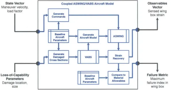
Similar to a living organism, an autonomous vchicle benefits not only from awareness of its surrounding environment and mission directives, but also from awareness of its performance capability. Because this degrades over time due to fatigue and acute damage, onboard logic often uses conservative estimates of performance from the initial vehicle design to plan feasible mission trajectories. We develop an approach for dynamically estimating vehicle capability to enable safer and more efficient mission planning. The approach leverages multi-level vehicle models in an offline phase to construct a library of in-formation capturing the vehicle behavior in damage scenarios; the behavior is discovered via data-driven classification techniques. After construction, the behavioral library is stored for future queries online by an agent making time-constrained decisions. The research directly links onboard vehicle sensor mea-surements with an estimate of the current vehicle maneuvering capability using the stored behavioral library.

The end-to-end process is implemented and demonstrated in an example flight scenario where an aircraft sustains structural damage to its wing. Safety is assessed based on composite material failure allowables, representing damage to the wing via a local loss of material stiffness. Damage scenarios on the wing are simulated and stored for query during the flight scenario, where knowledge of the maximum maneuvering load factor is estimated using structural strain sensor measurements. Results indicate both an increase in probability of suc-cess as well as an increase in overall usage of the vehicle capability, compared to the baseline case that does not dynamically update the capability with onboard sensor information.

Thesis Supervisor: Karen E. Willcox

Acknowledgments

I would first like to thank all those who supported me in undertaking this

research.

My advisor, Dr. Karen Willcox, has been an inspiration and guiding

force for me through the academic endeavor of engineering research as well as through the often equally important endeavors toward personal accomplish-ment, self-confidence, and a sense of earnestness in all of life's travails. My sincerest thanks and gratitude goes out to her.

I send my heartfelt thanks to Dr. Ella Atkins, who was a mentor and a source of guidance during my decision to go boldly forth to begin this research at MIT.

I would like to thank the members of the DDDAS project. At MIT, thank you to Laura, Demet, and Doug for their support in this work; and at Aurora Flight Sciences, thank you to David and Jeff for providing their expertise and guidance in the realm of aircraft structural composites (and all things practical about aircraft modeling).

I would also like to acknowledge the funding for this research, supported by AFOSR grant FA9550-11-1-0339 under the Dynamic Data-Driven Application Systems (DDDAS) Program (Program Manager Dr. Frederica Darema).

An aerospace graduate student's life at MIT is spent often in the labyrinth of externally concrete, internally leaking, yet somehow destruction-resilient research laboratory space we call home. I express my warmth for all the members of the Aerospace Computational Design Laboratory who shared this abode with me, both during our peaceful hours in the confines of Building 37 as well as during our less peaceful hours climbing stairs to prepare for Tough Mudding with Karen!

Beyond the laboratory space, my experience will forever remain a gem for the friends I have made at the Institute. Festivus Miracles, you hold the deed to a carefully tended vineyard in my heart, continuing to produce rich bottles of wine that will only ripen and grow in complexity with age. To Margaret, you are a radiance in my life, and this thesis bears the fruit your dedication and support has sowed.

Lastly, I want to express the breadth of my love for my family, who has empowered me to sculpt my identity and to make them proud. To my mother, father, and my sister Danielle, you are my persistent and guiding role models.

I know your love has been always near and this work is testament to your

Contents

1 Introduction

1.1 Origins of Dynamic Flight Capability Estimation 1.2

1.3 1.4

What is Capability Estimation? . . . . Research Objectives. . . . . Thesis Outline. . . . .

2 Methodology

2.1 Offline Phase . . . . 2.1.1 Step one: characterize system . . . .

2.1.2 Step two: classify behavior . . . .

2.1.3 Step three: construct library . . . . 2.2 Online Phase . . . . 2.2.1 Notation and assumptions . . . . 2.2.2 Inference using the maximum likelihood

2.2.3 Inference using a mixture distribution . .

2.3 Sum m ary . . . .

3 Aircraft Capability Model

3.1 UAV Aircraft Design . . . . 3.2 Aircraft M odel . . . .

3.2.1 Model configuration . . . . 3.2.2 Model validation . . . .

3.2.3 Lumped damage representation . . . . .

3.3 Wing Box Model . . . .

3.3.1 Local damage representation . . . .

3.3.2 Integration of VABS with ASWING . . . . . 3.4 Integrated Aircraft Capability Model . . . .

4 Classification, Application, and Results

4.1 Discovering the Capability Set Boundary via Cl assification

13 . . . . 13 . . . . 15 . . . . 16 . . . . 16 19 . . . . 19 . . . . 20 . . . . 21 . . . . 21 . . . . 22 . . . . 23 . . . . 24 . . . . 26 . . . . 28 29 . . . . 29 . . . . 31 . . . . 31 . . . . 32 . . . . 36 . . . . 37 . . . . 37 . . . . 41 . . . . 42 45 45

4.1.1 4.1.2 4.1.3

Support vector machines . . . . Probabilistic support vector machines . . . . Capability estimation using probabilistic support vector machines ...

4.2 Online Aircraft Capability Estimation . . . . 4.2.1 Flight scenario . . . . 4.2.2 Library damage cases and maneuver bou 4.2.3 Visualizing the library . . . . 4.2.4 Flight scenario test cases . . . . 4.2.5 Online strain gage measurements . . . . 4.3 R esults . . . . 4.3.1 Comparison of estimator outputs . . . . 4.3.2 _{Flight scenario performance benchmark .} 4.3.3 Lim itations . . . .

nds

5 Conclusion

5.1 Summary of Results and Current Work . . . .

5.2 Future W ork . . . . 46 50 . . . . 52 . . . . 55 . . . . 55 . . . . 56 . . . . 57 . . . . 61 . . . . 63 . . . . 66 . . . . 68 . . . . 75 . . . . 82 85 . . . . 85 . . . . 86

List of Figures

2-1 Offline methodology . . . . 20

3-1 UAV concept for capability analysis . . . . 30

3-2 UAV concept represented in ASWING . . . . 31

3-3 ASWING configuration for pull-up maneuver analysis . . . . 33

3-4 ASWING pull-up maneuver analysis varying airspeed . . . . 34

3-5 ASWING pull-up maneuver analysis varying load factor . . . . . 35

3-6 Lumped representation of damage in ASWING . . . . 36

3-7 Variational Asymptotic Beam cross-Sectional Analysis (VABS) flow chart . . . . 38

3-8 VABS damage representation demonstration . . . . 40

3-9 Wing cross sectional finite element model for VABS . . . . 41

3-10 UAV capability model coupling VABS and ASWING . . . . 42

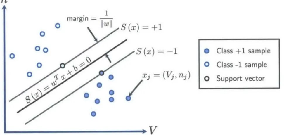
4-1 Description of a linear SVM discriminant . . . . 47

4-2 Refinement of PSVM vehicle capability estimate . . . . 54

4-3 Adaptive SVM convergence history . . . . 54

4-4 Schematic of the flight scenario to which we apply our capability estimation framework. . . . . 55

4-5 Offline library damage cases . . . . 57

4-6 Capability analysis region of aircraft maneuvering V - n envelope 58 4-7 Damage case PSVM countours . . . . 59

4-8 Visualization of vehicle behavioral library with representative cases ... ... 60

4-9 Choice of example damage cases . . . . 62

4-10 Strain sensing locations on aircraft wing box . . . . 64

4-11 Explanation of the probability curve plots used for analysis of qML and qMD- The vehicle state is x = (V, n), however V stays fixed at 210 ft/s so we need only plot the value of n. . . . . 67

4-12 qML output varying sample accumulation NS . . . . 69

4-14 Library down-sampling procedure controlled by DSR . . . . . 72

4-15 qML output varying library down-sampling ratio DSR . . . . . 73

4-16 qMD output varying library down-sampling ratio DSR . . . . 74

4-17 How an agent uses the capability estimation output via Pop . 76

4-18 Samples of decisions made based on the dynamic and capability estimation strategies, varying pp and n'tatic . . . . 78 4-19 p (MS)-n-,,tj trade-off curves for flight scenario decision

List of Tables

4.1 The five representative damage cases used in the flight scenario to test capability estimation performance. . . . . 61

4.2 Truth reference nmax values for five example damage cases . . 62 4.3 Damage case strain values for the fixed flight scenario maneuver 65 4.4 Numerical results obtained from the p (MS) -

nuti,

tradeoff

curves for the decision process using the static and dynamic capability estimation strategies . . . . 82

Chapter 1

Introduction

Modern aerospace vehicles are becoming increasingly independent of human interaction in-flight. Following this trend, a spectrum of technologies exist ranging from unmanned-vehicles that do not require a human operator in an airborne position but may require real-time interaction remotely via a pilot on the ground-to autonomous-vehicles that are able to make in-flight mission-critical decisions and react to stimuli in the environment. A mission-critical method for furthering autonomy is to produce self-aware systems: not only can these systems plan and operate independently of human operators, they are also able to quantify the state of their available internal resources and maintain knowledge of their current health beyond their initial baseline performance

[1].

In this way, the system mimics behavior of a biological organism-it can act aggressively when it is healthy and in favorable conditions, and can become more conservative as it ages and degrades.

In order to dynamically assess vehicle capability and use it to support autonomous operation, we need to develop an estimation process that can translate measurable quantities directly into capability quantities of interest. Especially as vehicle dynamics become increasingly complex, modeling this relationship is non-trivial when the computation needs to run within time constraints dictated by free flight.

1.1

Origins of Dynamic Flight Capability

Es-timation

The methods and tools for dynamic capability estimation have emerged from an intersection of work in both the vehicle damage detection and vehicle design communities.

Disciplines such as Operational Loads Monitoring (OLM) have worked to improve the detection of damage and fatigue in vehicle structural members. In OLM, on-board aircraft sensors gather structural loading information to identify damage and fatigue (most often post-flight) in order to reduce main-tenance costs and increase reliability [2, 3]. On a broader systems level, the Integrated Vehicle Health Management (IVHM) field searches for frameworks that incorporate multiple sources of operational data, physics-based models, and prognosis techniques [4, 5]. Modern IVHM architectures have been de-veloped at NASA [6] and the Department of Defense [7]. Damage and fault tolerance are now becoming an important component of real-time software ar-chitectures for monitoring aircraft component health, such as that proposed by the ONBASS project [8]. IVHM has also begun to enter the initial aerospace vehicle design where unit costs are high, and optimization techniques have been explored to improve IVHM architectures

_[9].

In addition to systems-level health monitoring, there has been active work on the vehicle component level, particularly in structural composites. Struc-tural Health Monitoring (SHM) using statistical inference techniques has seen active progress. Ref [10] presents a broad survey of the SHM field up to 2001, and recent work has approached damage detection problems using pattern recognition techniques [11]. Damage identification based on structural vibra-tion data has had particular success [12], where changes in vibravibra-tion modal fre-quencies often denote acute material degradation. More recently, high-fidelity modeling can enter into the damage identification and health management control loop-candidate models of system behavior can be weighted based on real-time data, and actions can be performed to increase estimation confidence, as well as actions to "heal" the system given current damage estimates [13].

However, work still remains to connect damage parameter identification to the online estimation of quantifiable vehicle capability. There is a need for global metrics used during the design phase-that drive the performance requirements of the vehicle-to be tracked and updated throughout the vehi-cle's lifetime. Standard design principles for aircraft operate on systems-level analyses such as the V - n diagram [14], where large margins of safety (often based on empirical evidence and experience) are substantial drivers for system efficiency. Recent work in condition-aware aircraft maneuverability [15] is advancing this connection, however open questions exist in how to integrate recent advances in local damage identification with updates to global aircraft performance metrics-forming this connection will improve usage of assets through their lifetime and could enable designs that rely on their dynamic usage in the presence of degradation.

1.2

What is Capability Estimation?

The word capability has a broad definition across engineering disciplines. In our context, we want to develop a quantitative definition so we can apply mathematics to the process of estimating capability for a given system.

To begin however, we must first define the concept of a system's state. We parallel the standard approach taken by the control systems community, where the state is a minimum number of quantities that, when considered together, can uniquely specify all possible configurations of the system [16]. To illustrate this concept, we describe three example systems and possible ways to characterize their state spaces:

1. A valve, with a single discrete state variable that designates whether it

is "open" or "closed."

2. An audio speaker "cone" that produces sound waves via linear res-onation, with its state quantified by its position and linear velocity.

3. A rigid-body aircraft in free flight and motionless air, with its state

quan-tified by the following degrees of freedom of a reference frame attached to a fixed point on its body:

e position and velocity with respect to a fixed Earth frame

* rotational orientation and velocity with respect to a fixed Earth

frame

Using this state vector with physical laws, we can predict how the motion of the aircraft will evolve in time due to inertial and aerodynamic loads; hence, its current value also uniquely identifies the aircraft configuration for future time instances

Now, we define the capability of a system quantitatively as the set of state vectors that satisfy constraints due to system properties or properties of its surrounding environment. We will also use the term capability set interchange-ably to reinforce the notion that the system capability is a set-valued quantity. For our three examples, the capability set could be interpreted as follows:

1. The capability set for a valve is normally both positions "open" and

"closed"-however due to a malfunction, the valve could be stuck in one position, and its capability set would shrink to a singleton with this position as its only element.

2. Due to actuator saturation and structural durability constraints, the audio speaker cone could have maximum displacement and maximum speed limitations during operation; the capability set would be the pairs of displacement and velocity bounded by these constraints.

3. Due to airframe structural failure and aerodynamic stall over the wings,

the aircraft could have constraints designating safe airspeeds and angles of attack with respect to the local air mass. The structural constraints could vary due to both local damage events, or due to changes in the environment such as temperature.

While our definition of capability is general, we focus in this research on quasi-static vehicle capability. Our methodology and application aim particularly at a system with continuous state variables, without explicitly analyzing the dynamic evolution of said state variables in time. However, the vehicle operates with time constraints on computation during operation that make high-fidelity modeling difficult, so we remain cognizant of the computational requirements of our approach.

1.3

Research Objectives

The broadest goal of this thesis is to present a method for performing online vehicle capability estimation leveraging computationally-intense, offline vehicle behavioral modeling. This goal is segmented as follows:

1. Develop a method for computing a library of system behavior using

physics-based models of the vehicle behavior in loss-of-capability scenar-ios.

2. Develop a computationally efficient technique for estimating vehicle ca-pability directly from noisy sensor information leveraging a pre-computed library of system behavior

3. Demonstrate the use of online vehicle capability estimation by an agent

in a scenario where the vehicle degrades, and compare its performance to the case where the agent only knows the nominal capability given by the vehicle design.

1.4

Thesis Outline

Chapter 2 introduces the methodology for using offline physics-based modeling to build a library of vehicle behavior, and for leveraging the library online to estimate vehicle capability.

Chapter 3 develops a representative UAV model that can capture its be-havior in the event of structural damage to its wing.

Chapter 4 applies the methodology from Chapter 2 to the representative

UAV from Chapter 3, presenting the algorithms used to implement the

capa-bility estimation process and results from a relevant decision-making process. It compares results to a baseline case that uses no active capability estimation, with detailed discussion.

Chapter 5 provides a summary of results, draws conclusions, and suggests directions for future improvement.

Chapter 2

Methodology

Our approach to flight capability estimation relies on a decomposition of com-putational effort between offline and online phases. The offline phase occurs before operation of the system of interest, when we assume we are able to leverage powerful computational environments that have relaxed execution time and storage constraints. The online phase refers to the real-time (or sim-ply time- and memory-constrained) parts of system operation, when embedded computation needs to be lightweight. We utilize complex physics-based mod-els, experimental data, and other sources of information about the system in the offline phase to build approximations of the system behavior; the approxi-mations can then run in the online phase to improve performance, for example by informing priors on quantities of interest or by enabling reduced-order mod-els of the system trajectory.

2.1

Offline Phase

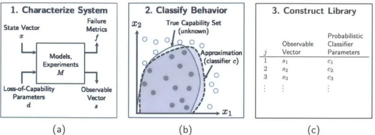
Figure 2-1 presents a functional decomposition of the offline phase of our methodology for estimating vehicle capability. The process is broken into three stages: characterization of the vehicle using models and/or experiments, sification of vehicle behavior based on failure modes, and storage of these clas-sifiers as records in a behavioral library. The following sections step through these stages in further detail.

1. Characterize System

Failure

State Vector Metrics

2~ f Models, ExperimentsI M _-Loss-of-Capability Observable Parameters Vector d a (a) (b) (c)

Figure 2-1: The three steps in the offline phase for building a library that can be queried in the online phase.

2.1.1

Step one: characterize system

Figure 2-la shows the first step-the user begins with vehicle system models and/or experiments that represent the vehicle behavior. They have two inputs and two outputs, the definitions of which are as follows:

* a state vector x E X, or any quantities that specify the configuration of the vehicle before considering changes to capability. For a maneuvering aircraft, x could be the kinematic state vector-for instance, in Chapter 4 we consider an aircraft in steady flight with a state quantified by an airspeed and a wing load factor, where X = R2

" loss-of-capability parameters d E D, or any quantities that specify how the vehicle could become modified such that its capability set would change-examples could be parameters describing structural damage, or parameters describing available system resources such as battery levels or fuel stores.

* A failure metric f : X xD -+ R that measures how close the vehicle is to undesirable or unpredictable behavior-examples could be closeness of structural loads to maximum thresholds, or closeness of available system resources to minimum safe levels.

" an observable vector s : X x D -+ S of quantities that would be available online to provide information about the vehicle state- for instance, in Chapter 4 we consider an aircraft with Ns continuous strain measure-ments provided by embedded wing sensors, where S = RNs.

2. Classify Behavior X2 True Capability Set

(unkn O) 0 0 0 00 Approimation 0 %(classifier c) mO₀ * ~ ,/0 3. Construct Library Probabilistic Observable Classifier j Vector Parameters 1 s₁ cl 2 82 C 3 83 C

2.1.2

Step two: classify behavior

The models and experiments produced in step one allow us to model the vehicle capability set as follows: if we represent a constraint on the vehicle behavior as an upper bound on the value of the failure metric f(x, d) for any input state x and loss-of-capability parameters d, then for a fixed value of d, the capability is the set of "safe" x's whose

f

values lie below this limit.

More precisely, let Kf be the upper bound on

f

that represents a constraint on the vehicle behavior. Then the capability set C is a function of d as follows:

C (d) = { E X : f(x, d) < Kf} (2.1)

This characterization of C as a set-valued quantity looks mathematically sim-ple, but it is difficult to use in practice. To make the problem tractable, we use a sampling-based classification technique to approximate C; the technique is represented conceptually in Figure 2-1b for a two dimensional, continuous state space X characterized by the coordinates (X1, X2). For each fixed value

of d, we generate samples from X and label them as "safe" (grey) or "unsafe" (light grey) based on whether they satisfy or do not satisfy, respectively, the predicate for set membership in C given by expression (2.1). Then, using the labeled samples, we train a classifier that is used to designate new query state vectors as "safe" or "unsafe." Because the classifier is trained off a finite set of samples, it can only approximate the true underlying capability set to some finite accuracy-but once we have the classifier trained, we could in the-ory use it to classify every point in the state space; this would produce the approximation of the capability set as shown (notionally) in Figure 2-1b.

We consider the possible discrepancy between our classifier and the true capability set a form of model error, and we introduce uncertainty to repre-sent this error. In particular, we train a probabilistic classifier for each value of d to evaluate the probability that a query state vector belongs to C(d). We perform the probabilistic classification for a given input x using the "proba-bilistic capability classifier quantities" c(d). For example, we implement this form of classification using a Probabilistic Support Vector Machine (PSVM) in Chapter 4, where c(d) contains quantities such as support vectors, weights, and distribution hyperparameters.

2.1.3

Step three: construct library

In step two, we approximated the capability set for each value of the loss-of-capability parameters via sampling-based classification. Now, by combining

the samples produced from these runs, we produce a library of records con-taining the following features:

" x, a value of the system state vector

" d, values of the system loss-of-capability parameters "

f,

a value of the system failure metric

" s, _{a value of the system observable vector}

* c, values of the probabilistic capability classifier quantities

We let R represent the number of records in this library, and we assign sub-scripts to denote these features for a given record

j

= 1, ... , R as xj, dj,

fj,

sj, and cj.

As a final, third step, we store this library for later queries in the online phase, as represented in Figure 2-1c. As we will show in the next section, the only features necessary for queries in the online phase are the observable vector s and the probabilistic classifier parameters c; the vehicle state and the loss-of-capability parameters are "hidden data" that were necessary only for modeling of the vehicle behavior. Essentially, our stored library will contain records that provide a direct link from vehicle observable quantities to vehicle capability.

2.2

Online Phase

In the online phase, the user directly infers the vehicle capability from an input sample of the vehicle observable vector, by use of the stored vehicle behavioral library. There are two intertwined classification steps involved:

1. The observable vector sample is used to classify the current vehicle

be-havior into cases represented in the library. We formulate this classifica-tion in a Bayesian sense, where the goal is to minimize the probability of misclassification.

2. Using the probabilistic classifiers that were pre-computed and stored for each record in the library, the user retrieves the probability that a query vehicle state lies within the current capability set.

The following sections introduce the process in a mathematical sense. We begin with a description of relevant notation, and then we present two possible methods for the inference process: a maximum likelihood formulation, and a mixture distribution formulation. The performance of these two methods will be compared later in our aircraft application in Chapter 4. Because the online

phase needs to be cognizant of available computational resources, we analyze the complexity of each method and discuss its implication with respect to the method's practical usability.

2.2.1

Notation and assumptions

As we will be working with probabilistic quantities, our convention is to denote random variables or vectors using serifed letters (e.g. a, b, and s), and to use shorthand, where values taken by random variables are represented by corre-sponding unserifed letters (e.g. a, b, and c). We represent probability mass and probability density functions as p

(),

where the corresponding discrete or continuous case will be clear from context. We represent the expectation operator as E [.]. In the event the random variable shorthand is ambiguous, we will revert to a subscript notation, so for example Pa (a) and p (a) both rep-resent the probability (or probability density, if a is continuous) that random variable a takes the value a.

We assume quasi-static vehicle behavior, where for any instant in time the vehicle state takes some value x

C

R'. By definition (2.1), the vehicle

capability is a set C C R'.

The models and/or experiments from the offline phase allowed us to build a library of information about the vehicle behavior. Here, we refer to each library record as representing a vehicle behavioral case, or a distinct shape of the vehicle capability set; note this is distinct from the vehicle state.

The notation for features of each record in the library follows that from section 2.1.3, where the Jth record for

j

= 1, ... R contains

" a value of the vehicle observable vector sj, containing Fs elements, and " a probabilistic classifier described by a vector cj of FC elements.

Each cj allows us to compute the probability that a query state x' lies in the capability set corresponding to the jth behavioral case. For notational

convenience, we define an indicator event Dj to designate whether the vehicle exists currently in the behavioral case represented by the jth library record, so that this probability can be written as p

('

C CI D). The Dj's are mutually exclusive, i.e. the vehicle can be in at most one behavioral case at any point in time; however, this does not mean the the vehicle is guaranteed to be in any of the library behavioral cases.

We assume the vehicle has a means of measuring the values in the observ-able vector s; we denote the random vector corresponding to these

measure-ments as

s.

Given the vehicle is in the j'" behavioral case,

s

has the form

s = s3 + e, (2.2)

where e is a random vector representing measurement noise that is independent of the vehicle behavioral case. We assume the user has knowledge of the statistics of e (often for physical systems it is characterized using a multivariate Gaussian with known mean and covariance), i.e. we can compute Pe (e), as well as

p (s ID ) = Pe (^ - s,) (2.3)

The goal of our inference process is to evaluate the vehicle capability given a measurement of the observable vector s. Because the vehicle capability is a set, one means of performing this task is to evaluate set membership, as introduced in Section 2.1.2. That is, we desire to evaluate a function q : X x S -+ R that closely approximates the probability of a query state x' C X lying within C given we observe S = s, i.e.

q (x', S) ~ p (x' E C Is) (2.4)

We develop two different formulations for q in the following sections, and add subscripts to identify them-the maximum likelihood variant qML is de-scribed in Section 2.2.2 and the mixture distribution variant qMD is dede-scribed in Section 2.2.3.

2.2.2

_{Inference using the maximum likelihood}

A straightforward means of obtaining an estimate of whether a state x' lies

in the vehicle capability set is to find the library record that maximizes the likelihood of the measured vehicle observable vector, and to then use the prob-abilistic classifier stored in that record to label x'.

Given our noise model in equation (2.2) for the measured observable vector, we can form the log-likelihood

f

(Dj ^) = log p (AIDj) = log pe (A- s j) (2.5)

of seeing measurement s given our vehicle is in the jth behavioral case stored in

our library (note that while sj was computed using values of the vehicle state and loss-of-capability parameters, these need not be known or represented explicitly here). We then maximize expression (2.5) over all possible values in

the library:

jmax = arg max f (Dj IS) (2.6)

jEl...R

Our maximum likelihood estimator, qML, is then the output from the proba-bilistic classifier corresponding to the (jmax)th library record:

qML (X, s) = p (x E CIDjma ) (2.7)

This process is agnostic of any prior over the records in the library, and simply seeks to find the record that "best explains" the measurements.

Time complexity

The time complexity of the Bayesian classifier can vary significantly depending on the application. Duda, Hart, and Stork [17] present a detailed analysis for the case where the noise model is a multivariate Gaussian-we present an ab-breviated form here. In our case, the Jh record of the lookup table represents a distinct class where the output noise model for said class is p (-I s) -

K

(sj, E) for some known covariance matrix E.

The complexity follows from equations (2.5)-(2.7):

1. Computing the log-likelihood f (sj Is) (equation (2.5)). For the multivari-ate Gaussian case, the likelihood of seeing output s from class

j

takes the following form:

1 d 1

2(sys) =- 2 ~ -- log 2r - -log|Zl (2.8)

(j^ 2 ( -s) P-s)-2 2

Given each sensor vector has Fs elements, computation of s - sj is

o

(Fs) and multiplication by E-- is 0 (Fl) (computation of E-1 only need be performed once and does not grow with Fs). Overall, the total complexity is approximately 0 (Fj).

2. Maximization of the log-likelihood (equation (2.6)). We perform this operation over the list of likelihoods for each record (i.e. each class) in our library-the worst-case time complexity for maximization over an unordered list of n elements is 0 (n), so our complexity is 0 (R).

3. Capability parameters lookup (equation (2.7)). Following the

maximiza-tion, we wish to access cimx of our library. Assuming we can read the jth

vector when computing the likelihood f (sj IS)- we need not include it in the complexity analysis here.

In summary, the time complexity of the Bayes classification process assum-ing a Gaussian noise model for a sassum-ingle output sample grows as ~ 0 (RFs). Our particular application assumes an arbitrarily large library, making R an important component of the time complexity growth.

Space complexity

The storage requirements for the maximum likelihood classifier grow only with the initial size of the library, i.e. as ~ 0 (R(Fs

+

Fc)).

2.2.3

Inference using a mixture distribution

As opposed to the maximum likelihood formulation that uses information from only the most-likely behavioral case in the library, it seems natural to design an estimator that combines information from each behavioral case, where more likely cases have more "influence" on the overall estimate than unlikely ones. We will first derive the mathematical form of the mixture distribution

estima-tor qMD, and then look into the mathematical form as a way of explaining the

reason behind the "mixture distribution" naming convention.

Observing expression (2.4), we can manipulate the right-hand and express it as a summation using the Law of Total Probability:

R

p (x' E CIS) ~ 1 p (Djls) p (x' E CID, S (2.9) j=1

The expression is an approximation because it relies on an assumption that j_1 p (D

[S)

= 1, i.e. that our current vehicle behavioral case is contained

somewhere in the R records in our library. This is a rough approximation that becomes increasingly accurate as our library becomes larger and richer.

Now, when conditioned on Dj,

{x'

E C} is independent of

{S

= S} because

our sensor noise is assumed to be independent of the vehicle behavioral case (see equation (2.2)). So, we can drop the conditioning on S^ on the right-most term inside the summation on the right-hand side of equation (2.9); applying Bayes' Rule, we obtain a final expression for our mixture distribution estimator

qMD (XI S):

R p(SIDj) p (Dj) _(.0

qID XRlp) p (x' E: C IDj ) (.

qMD _1 _{(^_ (sD j ) p (D y)I}

Note that the right-most term in the right-hand side summation is the value of each behavioral case's probabilistic classifier for the query vehicle state x'; in addition, the parenthetically-grouped term in front is essentially a normalized "weight" term. So, qMD can be interpreted as a weighted sum of the predic-tions that would be made by each record individually in the library were we to assume the vehicle was in each record's behavioral case. Probability distri-butions of this form are called "mixture distridistri-butions," where they are derived as a weighted summation of the distributions of distinct, underlying random variables -these underlying variables are often called "mixture components" and their weights are often called the "mixture weights." This is what provides the motivation behind the naming of the qMD estimator.

The "weight" term on the right-hand side of equation (2.10) requires knowl-edge of p (Dj), the a priori probability that the vehicle is in the jth behavioral

case. In Chapter 4, we choose to set p (Dj) as a maximum-entropy, uniform prior over all

j,

however the user could choose to use a different distribution to encode domain-specific prior knowledge about the vehicle behavior.

The power behind the mixture distribution estimator is an ability to closely approximate p (x' E CIS) despite the assumption that the vehicle behavioral case lies within our library of records. Intuitively, the capability set of a be-havioral case that is similar to several in the library, but not actually recorded in the library, could be "interpolated" via this weighting of the capability sets of nearby library records. However, this method comes at added computa-tional cost compared to the maximum likelihood estimate, as is shown in the following sections.

Time complexity

We can perform a complexity analysis similar to the maximum likelihood

clas-sifier complexity as presented previously, using a multi-variate Gaussian noise model. By re-writing Eq. (2.10) as

Ej=1 p (SIDj) p (Dj) p (x' E C IDj)

we see the computation involves two parallel summations over 1... R entries. The process can be broken down as:

1. Computing p (81 Dj). This is of the same order as computing the log-likelihood for the maximum log-likelihood classifier, 0 (FS).

2. Computing p (x' E _{CIDj). Unlike for the maximum likelihood classifier,}

we must evaluate the capability boundary for each lookup table record. This will play an important role in the increased overall complexity-for now, let us suppose this complexity is some function Oc(R, Fc) that is of reasonable polynomial order.

3. Summation over all lookup table records 1... R. The summation is of

the order 0 (R) similar to the complexity of performing arg max for the maximum likelihood classifier.

In summary, the time complexity of the mixture model classification process grows as 0 (RFSOc(R, Fc)), where Oc(R, Fc) the complexity of performing a single capability boundary evaluation.

Space complexity

Just as for the maximum likelihood classifier, the storage requirements for the mixture model classifier grow only with the initial size of the lookup table, as

~ 0 (R(Fs + Fc)).

2.3

Summary

We have developed and presented our methodology for estimating vehicle capa-bility in a quasi-static manner, using a measurement of vehicle observables-with a priori noise model assumptions-to estimate the probability that a query vehicle state lies within the current capability set. The methodology comprises an offline stage where we can use physics-based models and ex-periments to build and store a library for use in an online phase. We have presented two techniques for capability estimation in the online phase, and quantified their complexity with respect to the dimensionality of the stored data.

Chapter 3

Aircraft Capability Model

We apply our data-driven capability estimation methodology to the case of a representative UAV with mission performance affected by in-flight structural degradation. We present the UAV design in Sections 3.1; next, we present the development and validation of a global medium-fidelity model of the UAV Section 3.2 and a local high-fidelity wing box model in Section 3.3. Lastly, we present the top-level integrated model hierarchy in Section 3.4.

3.1

UAV Aircraft Design

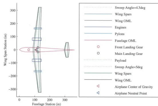
The UAV design evolved from a first-principles sizing routine [18] and Federal Aviation Regulation (FAR) 23 guidelines. As shown in Figure 3-1, the vehicle has a wing span of 55 ft. It is designed to cruise at 140 kn (240 ft/s) at an altitude of 25, 000 ft. The fuselage accommodates a payload of 500 lbs. The estimated range of the aircraft is 2500 nmi, corresponding to a flight duration of approximately 17.5 hrs. This allows for adequate operational capability to explore maneuverability as a function of the changing structural state of the vehicle.

100 200

Fuselage Station (in)

300 ... Sweep Angle=4.3deg Wing Spars Wing OML Engines Pylons Fuselage OML

o Front Landing Gear

o Main Landing Gear

Payload

. ... Sweep Angle=5deg

Wing Spars Wing OML

Airplane Center of Gravity Airplane Neutral Point

Figure 3-1: A realistic concept unmanned aerial vehicle established to estimate the effect of structural degradation on capability.

300 200 100 -0 0 100| -200 -300-0 -F

3.2

Aircraft Model

Aero-structural loads on the UAV are estimated using ASWING [19], a nonlinear aero-structural solver written in FORTRAN for flexible-body aircraft configura-tions of high to moderate aspect ratio. We use ASWING to predict internal wing stresses and deflections as a function of input aircraft kinematic states and estimates of damage to the nominal aircraft structure. Figure 3-2 shows the representation of our concept UAV in the ASWING framework. The ASWING model is a set of interconnected slender beams-one each for the wing, fuse-lage, horizontal stabilizer, and vertical stabilizer. Lifting surfaces (the wing and stabilizers) have additional cross-sectional lifting properties that are pre-specified.

Figure 3-2: The representation of our concept UAV within ASWING. The structure

is specified as a set of interconnected slender beams, where lifting surfaces have additional aerodynamic properties specified along their span.

3.2.1

Model configuration

ASWING is capable of static, dynamic, and modal analyses of airframes; how-ever, we only use its static analysis tools in this work. Specifically, we trim the aircraft to simulate "pull-up" maneuver conditions, where the nose is pitched upward to increase the wing angle-of-attack and wing load factor n = . This

maneuver is often used as a representative case of maximal structural loading conditions where, for a fixed airspeed, we can trim the aircraft to increasing values of n until either stall or structural failure occurs.

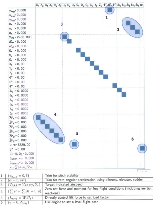
Figure 3-3 presents the internal ASWING constraint matrix used to configure the pull-up flight conditions. The user supplies a target value for the (indi-cated) airspeed, and then controls the trim load factor directly by specifying a target lift force in units of the aircraft gross weight.

3.2.2

Model validation

We validate the UAV representation in ASWING by trimming it to steady-level cruise conditions at a load factor n = 1 for a range of airspeeds above and below the nominal design cruise speed, and observing its response compared to expected behavior based on the (previously validated) aircraft design.

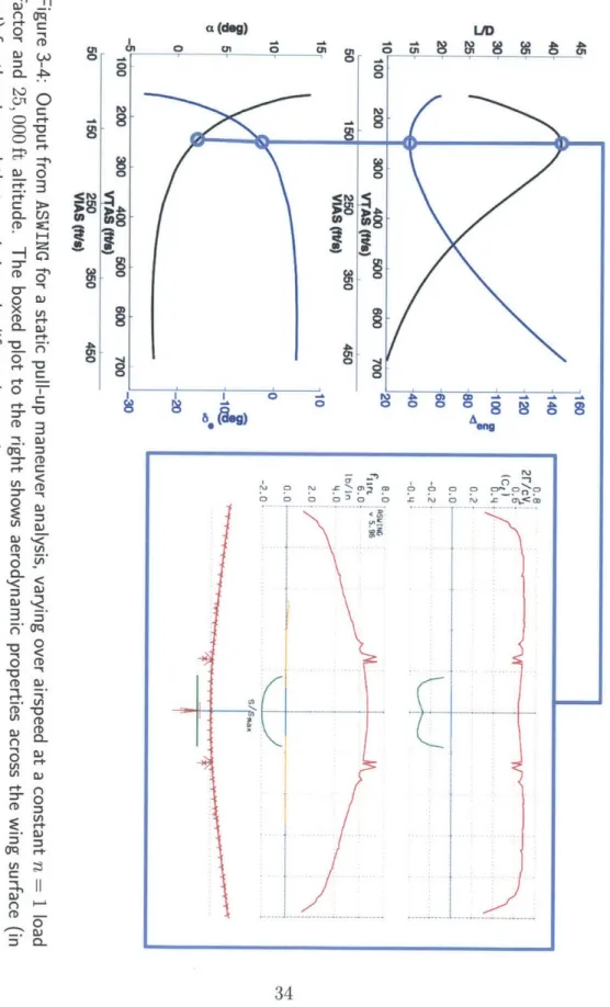
Figure 3-4 shows the lift-to-drag, engine setting, angle of attack, and eleva-tor setting obtained from this analysis, along with an example of the deflection profile across the wing surface in the blue-boxed callout (shown facing the front of the aircraft; the wing profile is drawn in red).

At cruise conditions, the airspeed that maximizes the UAV lift-to-drag is approximately 250 ft/s ~ 148 kn, which is a less-than- 6% change from the orig-inal design cruise speed of 140 kn. We consider this as acceptable agreement for continuing use of the ASWING model, especially given the UAV representa-tion in ASWING requires simplificarepresenta-tion of the geometry to interconnected beams with only 1-D span-wise lumped properties. We also attribute some error to some changes to the wing structure that were necessary to integrate with our high-fidelity beam model in VABS, described further on in Section 3.3.

After observing the n = 1 aircraft behavior, we fix the airspeed at the optimal cruise speed of 250 ft/s and observe the behavior of the model over increasing load factor n, shown in Figure 3-5. The aircraft is equipped with inboard high-lift flaps, that are activated to 150 to give an additional "bump" to the wing lift profile. This allows the aircraft to perform at higher load factors (in our case, this is quantified as in excess of 3G's) without stalling. Maneuvers at higher load factors are in the flight regime where the structural loading constraints become particularly important, so this regime is where we wanted to place our structural degradation analysis to have a relevant impact on the vehicle capability.

A a a a c y az UU Uz x () Oz XE YE ZE j $ 6F 6F₂6FN 6F a,, 0.000 az,, 0. 000 a. -0.000 aw -0.000 az -0.000 V1As -2438. 000 a**.r0. 000 0. -0.000 aw -0.000 Oz =0.000 XE =0.00 YE -0.00 ZE -0.00 $* -0.00 8* -0.00 *0 0.00 6FI 0.0000 6F2 -0000 6F3 0.0000 6r, =0.0000 6 F5 = 0. 0000 AEI -0.0000 Y-Fx -0. 000 0F -0. 000 =Fz -0. 000 =I .0.000 IMx- 0.000 MZ -0.000 LirL- 3229. 00 * -0.00 6Y -Ux 0Z -0. 000 Cuserj-u 0.000 Cuser2'u 0.000 mI n5 6-6, l/w 1 3

U..

\

5

6

1 (a. = 0, 0) Trim for pitch stability

2 (a = 0, F) Trim for zero angular acceleration using ailerons, elevator, rudder

3 (VrAs = VSPEC, U.) Target indicated airspeed

4 (E F = E M = 0, a) Zero net force and moment for free flight conditions (including inertial reactions)

5 (Ln=1 = W, Uz) Directly control lift force to set load factor

6 (y = 0, Aeng) Use engine to set a level flight path

Figure 3-3: Snapshot of the ASWING constraint configuration menu for a static pull-up maneuver analysis. ASWING attempts to satisfy the constraints given in the matrix to the left when trimming the aircraft. A turquoise box indicates the flight state variable in the corresponding row is constrained to its assigned value by the variable in the corresponding column. The table to the right gives additional

explanation for select groups of constraints in the matrix.

150 300 400 500 600 700 VTAS (ftM) 250 VIAS (fts) 160 140 120 100 60 40 350 460 100 200 300 400 500 600 700 VTAS "a) 50 150 250 350 ViAS (ftfs) 10 0 -20 -20 0.8 2r/cv 0.2--30 450 Figure 3-4: Output from ASWING for a static pull-up maneuver analysis, varying over airspeed at a constant n = 1 load factor and 25, 000 ft altitude. The boxed plot to the right shows aerodynamic properties across the wing surface (in red) for the airspeed that maximizes the lift-to-drag ratio. 45 40 35 25 20 15 In 100 200 50 15-10 -0.2--0.4. 5-0 I ~ ... .. ... ... LAMMERS= 0.0 01 4.0 2. 0.0o ASWING S. 96 max

1.4 1.8 2.2 2.6 Load Factor 3 3.4 10 5 0 -15 -20 -25 -30 2.0I 2r/c. (C .. 0.0 Lift "bump due to 0t5 L0_ activation of flaps 30.0 2D.0 _lb/In 10.0- 0.0. Figure 3-5: Output from ASWING for a static pull-up maneuver analysis, varying over load factor at a constant airspeed of 250 ft/s and a constant altitude of 25, 000 ft. The boxed plot to the right shows aerodynamic properties across the wing surface (in red) for n = 2, i.e., for a maneuver that loads the wing with twice the gross weight of the aircraft. 15 10 5 I I OF -5 ."1 I

max

ASWING SAG --- --

---3.2.3

Lumped damage representation

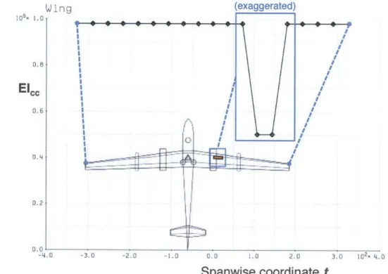
To modify the maneuvering capability of the aircraft, we represent tural degradation due to damage on the aircraft wing. The ASWING struc-tural members, as slender beams, consist of span-wise beam stiffness property distributions-one means of representing damage is by a reduction in these beam stiffness properties. Figure 3-6 demonstrates this in the case of the wing bending stiffness along an axis parallel to the wing chord, EIce (i.e. the wing bending stiffness that is related to "flapping" or the most visible U-shaped deflection of the wing); the reduction is greatly exaggerated in the figure for explanatory purposes. We leave the aerodynamic properties of the model un-touched by our damage representation; hence for a given trim condition the aerodynamic loading will change purely via coupling with the modified struc-tural properties. (exaggerated) 109 1.0 0.0 -4.0 -3.0 -2.0 -1.0 0.0 1.0 2.0 3.0 102x 4.0 Spanwise coordinate t

Figure 3-6: Illustration of how "lumped" damage effects could be represented in ASWING by reducing one-dimensional beam stiffness properties along their span.

ham-pers the wing's ability to carry structural loads through the affected region. However, it is too simplified-local damage to a wing structure will produce local stress raisers that are not visible to this lumped representation in ASWING. These local stress raisers are what we can directly compare to material allow-ables, to determine whether the damage causes unsustainable local stresses in the surrounding undamaged material. To account for these local stress raisers, we couple our ASWING model with a high-fidelity wing box representation. The next section describes the high-fidelity modeling technique and presents how we couple it with ASWING.

3.3

Wing Box Model

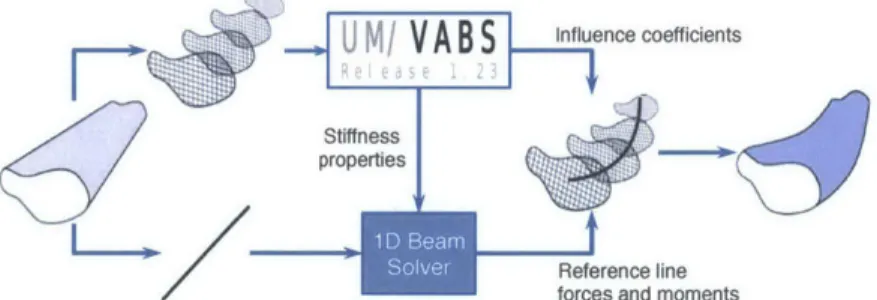
To resolve stiffness loss due to local damage on the aircraft wing, we need another technique to interface with the global ASWING aircraft model. In lieu of forming a three-dimensional finite element representation of the wing, we use Variational Asymptotic Beam Cross-Sectional Analysis (VABS) [20, 21], a powerful dimension reduction technique used in industry practice. A vi-sual representation of the VABS methodology is shown in Figure 3-7. To model a beam in VABS, the user first represents the beam as an array of two-dimensional cross-sectional finite element models. The cross-sections cap-ture the details of a multi-ply composite wing skin and local damage effects. VABS then computes lumped stiffness and inertial properties at a reference point in each cross section, forming a "global" line representation of the beam.

A one-dimensional beam solver can then find the global force and moment

distribution along this reference line given input forces and moments. Lastly, the user recovers the internal stress and strain fields using the reference line solutions and influence coefficients initially computed by VABS-the influence coefficients are linear transformations relating the reference line solution to the 3-dimensional stress and strain tensors in each element of the cross section.

In this work, we use the UM/VABS ri.31 implementation developed in FORTRAN by R. Palacios and C. Cesnik at the University of Michigan [22] (referred to hereon as VABS). Our beam of interest is the aircraft wing box, and ASWING manages the one-dimensional beam solution, computing loads in the wing box for specific flight conditions.

3.3.1

Local damage representation

Using VABS, we can represent structural modifications due to damage on a cross-sectional, two-dimensional finite element level. Each element in the

model represents a portion of composite material viewed through its thickness, containing material stiffness and angular orientation (i.e., ply angle) proper-ties. We represent damage as a reduction in the material stiffness properties of affected elements-the physical nature of this damage is general, as we do not do further detailed damage modeling (e.g., for crack propagation or composite delamination). However, our implementation is left open-ended to allow for future addition of higher-fidelity damage models that are compatible with the VABS technique.

As a first-order approximation, this damage representation allows us to observe the impact of local stiffness reduction on surrounding un-modified el-ements. The loss of stiffness in one region causes local stress raisers in nearby "healthy" elements, potentially causing premature failure in these nearby el-ements. We define whether a healthy element would fail under given loading conditions by looking at its internal failure indices, of the form cj /,qlowable

for i,

j

= 1, ... , 3; eij is the strain in the direction of material axis

j

on a

sur-face within the element whose normal points in the direction of material axis i, and 6qlowable is the corresponding allowable limit imposed by the material

properties. Thus, for each element there are 6 failure indices corresponding to failure in

* 3 directions due to normal strain failure (extensional or shear), and * 3 directions due to shear strain failure.

We then take a maximum over all the failure indices in every element of the cross section to obtain one single scalar value representing whether a failure would occur somewhere within the cross section. This is repeated for every cross section in the wing, and by taking another maximum we can obtain a

U M/ V AB

5

Influence coefficients

Stiff ness

properties

* - Reference line

forces and moments

Figure 3-7: Variational Asymptotic Beam Cross-Sectional Analysis (VABS) allows for dimensional reduction of an expensive three-dimensional beam solution into two-dimensional finite element models coupled with an external beam solver.

single scalar failure index representing whether failure would occur somewhere in the entire wing structure.

The material axes 1,2, and 3 are defined with respect to the fiber orien-tations in each of the material plies of the cross section, and hence they may not necessarily coincide with the axes system of the cross section (which by definition in UM/VABS ri.31 has its 1-axis point outward along the beam span, its 2-axis point to the right in the plane of the cross section, and its 3-axis point up in the plane of the cross section).

Figure 3-8 demonstrates this failure analysis on a cross section that is representative of a symmetric aircraft wing box (note that most wing boxes would have much thinner walls; this example has thicker ones for illustrative purposes). A damage event on the top surface causes an increase in the cross-sectional maximum failure index for a fixed loading condition (in this case, the loading is a pure moment about the Y-axis).

Undamaged IE REF I 0 2 4 6 8 Damaged dan Z

L

REF mage region R:0.975 CI UII W 0 2 4 6 8 Index

Figure 3-8: Output from VABS for an example cross section (with three plies oriented in a [00, 900, 00] stack) when under a pure Y-axis moment. Failure indices are plotted for both the undamaged and damaged cases-note that although no failure indices are computed in the damaged region, the material is still present in the FEM. 1 0.9 0.8 0.7 0.6 0.5 0.4 0.3 0.2 0.1 2 1 0 -1 -2 2 1 0 -1 -2

Higher failure indices on top surface because

material allowable is lower in compression than in tension 0" F: il r Local increase in failure indices in nearby undamaged material i , ftlffi 0.887

3.3.2 Integration of VABS with ASWING

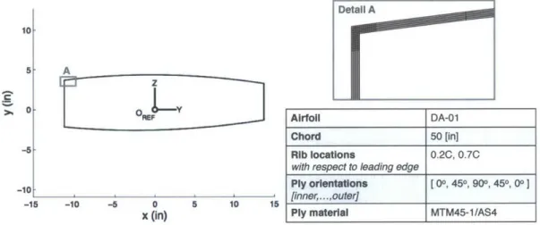
For integration with our aircraft model, we use a VABS cross-sectional FEM that matches the same airfoil shape as the ASWING model. For a given damage case, we run VABS to update the lumped mass and structural stiffness prop-erties for the wing representation in ASWING. Figure 3-9 shows the geometry of our VABS model for an undamaged configuration with a table of relevant properties. We only form a model of the wing box, as this carries the majority of the wing's structural loads (the ribs are at fixed locations with respect to the chord, and the top and bottom surfaces follow the airfoil outer contour).

Detail A 10-5- A 0 LY 5 - -10--15 -10 -5 0 5 10 15 x (In) Airfoil DA-01 Chord 50 [in] Rib locations 0.2C, 0.7C

with respect to leading edge

Ply orientations [00, 450, 900, 450, 00]

[inner,...,outer]

Ply material MTM45-1/AS4

Figure 3-9: Constant cross section finite element model used for VABS analysis, allowing refinement of stress raisers caused by local stiffness loss due to damage.

In addition, we use a constant cross section for our analysis to make the number of function calls to VABS computationally tractable. The chord length in the VABS model is an averaged value of the tapered chord distribution from the original ASWING model, while the tapered chord distribution was still re-tained in the ASWING model to provide realistic, efficient aerodynamic washout. However, this means the ASWING model uses a wing that (when undamaged) has constant structural properties but varying aerodynamic properties. The constant structural properties cause only a small change to the nominal aero-structural performance of the vehicle when compared to the initial design, as shown previously in Section 3.2.2.

Note that without the VABS technique, the aircraft model in ASWING would not be able to elicit a high-resolution material failure metric for a given damage condition, as the elevated material stresses are of a local nature. An alternative