Demographical Trajectories of European urban areas (1961-2011) (TRADEVE)

HAL Id: halshs-01311420

https://halshs.archives-ouvertes.fr/halshs-01311420

HAL is a multi-disciplinary open access archive for the deposit and dissemination of sci-entific research documents, whether they are pub-lished or not. The documents may come from teaching and research institutions in France or abroad, or from public or private research centers.

L’archive ouverte pluridisciplinaire HAL, est destinée au dépôt et à la diffusion de documents scientifiques de niveau recherche, publiés ou non, émanant des établissements d’enseignement et de recherche français ou étrangers, des laboratoires publics ou privés.

Demographical Trajectories of European urban areas

(1961-2011) (TRADEVE)

Anne Bretagnolle, Marianne Guérois, Antonin Pavard, Paul Gourdon, Natalia

Zdanowska, Liliane Lizzi

To cite this version:

Anne Bretagnolle, Marianne Guérois, Antonin Pavard, Paul Gourdon, Natalia Zdanowska, et al.. Demographical Trajectories of European urban areas (1961-2011) (TRADEVE). [Research Report] Université Paris 1 Panthéon-Sorbonne. 2016. �halshs-01311420�

Université

Paris 1

Panthéon-Sorbonne

(AAP 2014)

Anne Bretagnolle, Marianne Guérois, Antonin Pavard*, Paul Gourdon, Natalia Zdanowska, Liliane Lizzi UMR Géographie-cités, * Engineer in geomatics

Scientist Comittee : Emmanuèle Sabot-Cunningham, Sylvie Fol, Julia Salom, Manuel Wolff

Demographical Trajectories of

European urban areas

1

LIST OF AUTHORS

Anne Bretagnolle, University Paris 1 Panthéon-Sorbonne, UMR 8504 Géographie-Cités Marianne Guérois, University Paris-Diderot Paris 7, UMR 8504 Géographie-Cités

Antonin Pavard, Engineer in Geomatics (ant.pavard@gmail.com)

Paul Gourdon, University Paris 1 Panthéon-Sorbonne, UMR 8504 Géographie-Cités Natalia Zdanowska, University Paris 1 Panthéon-Sorbonne, UMR 8504 Géographie-Cités Liliane Lizzi, UMR 8504 Géographie-Cités

Contact

anne.bretagnolle@parisgeo.cnrs.fr

UMR 8504 Géographie-Cités Tel. (+ 33) 1 40 46 40 00

LIST OF SCIENTIFIC PARTNERS:

Emmanuèle Cunningham-Sabot, Ecole Normale Supérieure, Paris. Sylvie Fol, University Paris 1 Pantéhon-Sorbonne.

Julia Salom, University of Valencia, Spain

Manuel Wolff, Helmholtz-Zentrum für Umweltforschung (UFZ, Helmholtz center for environmental research), Leipzig, Germany

SCIENTIFIC COLLABORATION:

2

Table of Contents

I.

INTRODUCTION ... 5

II.

METHODOLOGY ... 6

A. Sources ... 6

1. Presentation of the different databases ... 6

2. Corrections of the LAU & Historical Populations Databases (1961-2011) ... 8

3. Adaptations of the LAU shapes 1961-2011 ... 10

B. Which models for following European urban areas on five decades? ... 11

1. Choice of an evolving delineation for European urban areas ... 11

2. Criteria and parameters for selecting urban building blocks ... 12

3. Construction of the task model ... 13

4. The resulting data model ... 14

C. Methodological implementation ... 15

1. Presentation of the tools ... 15

2. Rational choice of the 2000 inh. minimal threshold ... 17

D. Database validation ... 19

1. Spatial illustrations of evolving delineations ... 19

2. Statistical comparisons at national scale ... 20

3. Statistical comparisons at European scale... 22

III.

EXPLORATIONS OF THE RESULTING UMZ-TRADEVE DATABASE AT

THE EUROPEAN SCALE ... 22

A. Urbanization levels ... 22

1. North-Western Europe... 22

2. Atlantic and Mediterranean periphery ... 23

3. Central Europe ... 24

B. Urban growth ... 24

C. Urban hierarchy ... 30

D. Urban trajectories ... 33

IV.

URBAN TRAJECTORIES AT NATIONAL LEVEL FOR SELECTED

COUNTRIES ... 39

A. Germany ... 39

B. Romania ... 41

C. Spain ... 42

3

V.

FOCUS ON DECAY AND STAGNATION PATTERNS ... 44

VI.

CONCLUSION ... 45

VII.

REFERENCES ... 46

VIII.

ANNEXES ... 47

A. Historical Population Database: Computing specifications per country ... 47

B. Data Checking of the Historical Population database, per country ... 48

C. Minimal population threshold experiments ... 74

D. Minimal density threshold experiments ... 77

E. Total and urban Population (Tradeve-UMZ) per country ... 81

F. Inertia bar plots: How to cut the tree in the hierarchical cluster analysis on urban trajectories at European level ... 84

G. Hierarchical Cluster Analysis on Urban Trajectories of European Agglomerations presenting a decay or a stagnation profile ... 84

Figure II-1 : Dictionary of correspondence between LAU2 and UMZ 2000 ...7

Figure II-2 : Four models of time-integration in urban databases... 12

Figure II-3 : Four steps for constructing Tradeve urban areas ... 14

Figure II-4 : The TRADEVE data model ... 15

Figure II-5 : Extension of urban areas in Jutland (Denmark) ... 19

Figure II-6 : Extension of urban areas in Eastern Denmark (including Copenhagen) ... 19

Figure II-7 : Extension of Madrid (Spain) ... 19

Figure II-8 : Extension of Barcelona (Spain) ... 19

Figure II-9 : Extension of Lyon (France) ... 20

Figure II-10 : Extension of Paris (France) ... 20

Figure II-11 : Extension of urban areas in Czech republic ... 20

Figure II-12 : Rank-size graphs of French TRADEVE-UMZ and Unités urbaines... 21

Figure III-1 : Urbanization levels in North-Western Europe ... 23

Figure III-2 : Urbanization levels in Atlantic and Mediterranean countries... 23

Figure III-3 : Urbanization levels in Central Europe... 24

Figure III-4 : Population of urban areas in Europe (1961-2011, Tradeve-UMZ) ... 25

Figure III-5 : Average annual growth rate of Tradeve-UMZ (1961 to 2011) ... 26

Figure III-6 : Average annual growth rate of European urban areas between 1961 and 1971 . 27 Figure III-7 : Average annual growth rate of European urban areas between 1971 and 1981 . 28 Figure III-8 : Average annual growth rate of European urban areas between 1981 and 1991 . 29 Figure III-9 : Average annual growth rate of European urban areas between 1991 and 2001 . 29 Figure III-10 : Average annual growth rate of Tradeve-UMZ (2001-2011) ... 30

4

Figure II-13 : Degree of inequality of urban area sizes in Europe, Tradeve-UMZ (1961-2011)

... 31

Figure III-11 : Degree of inequality in urban area sizes, North-Western, Atlantic and Mediterranean Europe ... 32

Figure III-12 : Degree of inequality in urban area sizes, Central Europe ... 32

Figure III-13: Hierarchical cluster analysis on trajectories of Trdeve-UMZ (1961-2011) ... 33

Figure III-14: Relative weight of the four clusters ... 34

Figure III-15: Demographic trajectories of Tradeve-UMZ (1961-2011), urban surfaces ... 35

Figure III-16: Demographic trajectories of Tradeve-UMZ (1961-2011), urban patterns ... 36

Figure III-17: Demographic trajectories of Tradeve-UMZ (1961-2011), urban populations... 37

Figure IV-1: Demographic trajectories of German urban areas (1961-2011) (Hierarchical Cluster Analysis at the European level)... 40

Figure IV-2: Demographic trajectories of German urban areas (1961-2011) (Hierarchical Cluster Analysis at the national level) ... 40

Figure IV-3: Demographic trajectories of Romanian urban areas (1961-2011) (Hierarchical Cluster Analysis at the European level)... 41

Figure IV-4: Demographic trajectories of Romanian urban areas (1961-2011) (Hierarchical Cluster Analysis at the national level) ... 41

Figure IV-5: Demographic trajectories of Spanish urban areas (1961-2011) (Hierarchical Cluster Analysis at the European level)... 42

Figure IV-6: Demographic trajectories of Spanish urban areas (1961-2011) (Hierarchical Cluster Analysis at the national level) ... 42

Figure IV-7: Demographic trajectories of British urban areas (1961-2011) (Hierarchical Cluster Analysis at the European level)... 43

Figure IV-8: Demographic trajectories of British urban areas (1961-2011) (Hierarchical Cluster Analysis at the national level) ... 43

Figure V-1: Demographic trajectories and population 2011 of the European urban areas characterized by decay or stagnation (1961-2011)... 44

Tableau II-1 : Corrections added by the Tradeve project to Historical Population Database, per country (see files per country in Annex B for more details) ...8

Tableau II-2 : Total number of Tradeve-UMZ reconstructed for 2001 year according to different criteria and parameters ... 18

Tableau II-3 : Total number of Tradeve-UMZ per year according to different criteria and parameters ... 18

Tableau II-4 : Index of inequality sizes (absolute value of rank-size graph’s slope) ... 21

Tableau II-5 : Comparison between Tradeve-UMZ and Geopolis database (total number and inequality index) ... 22

Tableau III-1: Hierarchical Cluster Analysis outcomes by country (count) ... 38

5

I.

Introduction

TRADEVE project « demographical trajectories of European urban areas » (TRAjectoires DEmographiques des Villes Européennes) has been granted by University Paris 1 Panthéon-Sorbonne for the period 2014-2016. The aim of the project is to build a harmonized database on delineations and populations of European urban areas (defined by taking into account continuous build-up areas and minimal population threshold), from 1961 to 2011. More than 3900 urban areas (exactly 3946) are considered for 2011, for 29 countries (see the list in annexVIII.E). The different researchers that are involved in TRADEVE work specifically on urban geography and geomatics. Most of them have been involved in ESPON Database from 2008 to 2014.

In the TRADEVE project, we mobilised a harmonised database that allows studying small and medium urban areas, the Urban Morphological Zones (UMZ). Originally defined by the European Environment Agency from CORINE Land Cover images and continuous built-up areas criteria (Milego 2007), UMZ were poorly used for urban studies until they were enriched in the ESPON Database by other indicators, such as a name for each agglomeration and a correspondence dictionary with LAU2 that allows joining other statistical datasets. A population density grid from the Joint Research Centre (Gallego 2010) was used for attributing populations to these urban areas (Bretagnolle et al. 2016). This grid, with a resolution of 100 m, was constructed by using information from CORINE Land Cover in order to disaggregate LAU2 populations at a finer scale of observation (a weighting coefficient is attached to each category of land use and gives the share of the urban population to be reallocated). We also validated the use of the UMZ database by comparing urban populations or surfaces with those from national urban databases in Sweden, Denmark and France (Guérois et al. 2012). The UMZ database allows, in a comparable way, the study of all urban areas larger than 10 000 inhabitants. The Morphological Urban Areas (MUA) defined by Christian Vandermotten et al. (1999) are much less numerous, as their minimal threshold is 20 000 inhabitants: we find 1988 MUA instead of 3953 Tradeve-UMZ in 2000. The new Larger Urban Zones, delineated in a harmonised way by DG Regio, Urban Audit and OECD, are much fewer, using a minimal threshold of 50 000 inhabitants (Djijstra and Poelman 2012). Turok and Mykhnenko (2007) started from Cheshire’s database (1995) and tried to enlarge timespan, but only for cities larger than 200 000 inhabitants.

Section 2 focuses on the different methods that have been used for retropolating UMZ to 1961, by using and correcting for some countries the population data collections for the Local Administrative Units database on LAU2 population from Gloersen et al 2013 (Historical Population Database) and by populating the 2000 perimeter with 2011 data. In Section 3, different explorations of the resulting database are presented, for urban growth, urban hierarchy and demographic trajectories.

6

II.

Methodology

1. Presentation of the different databases Four different databases were used in the TRADEVE project :

(i) Local Administrative Units (EuroBoundaryMap, 2012 geometry) with Historical Populations Data for 1961, 1971, 1981, 1991, 2001 and 2011 (Gloersen et al. 2013).

(ii) Urban Morphological Zones 2000 (version v2) (see Bretagnolle et al. 2014)

(iii) Dictionary of correspondence LAU2/UMZ (restricted version, see Figure II-1) elaborated

in ESPON Database (see Bretagnolle et al. 2014) 1. It concerns UMZ 2000 and LAU2 (2012

geometry) and gives the different LAU2 that are linked to UMZ 2000.

1 _{Populations come from “Population density grid” estimated by Joint Research Centre (Gallego} 2010). When different UMZ are included inside one LAU2, they are aggregated.

7

Figure II-1 : Dictionary of correspondence between LAU2 and UMZ 2000

8

2. Corrections of the LAU & Historical Populations Databases (1961-2011)

The Historical Population database, constructed by Gloersen et al. (2013), can be downloaded on Eurostat website. This database has been constructed with fully detailed metadata which really facilitated its using. We first checked geometrical and statistical data and made different corrections, for instance by comparing results and extractions from national census boards (see below). Then we sent the final results to Erik Gloersen, who updated the datasets on Eurostat website.

The Historical Population database refers to LAU2 level, excepted for Greece, Portugal, Lithuania and Slovenia (LAU1). Data populations are computed for 1961, 1971, 1981, 1991, 2001 and 2001, in the 2012 administrative units. They have been interpolated at the 1st January of each reference year. The geometry generally comes from EuroBoundaryMap 2012, with some minor exceptions for Ireland and major exceptions for Greece (other sources, see Gloersen et al. 2013). Data have been processed by Erik Gloersen and Christian Lüer (Spatial Foresight) for 12 countries, and by national experts for the rest of the countries. Countries can be separated in 3 different groups, according to the kind of processing (Annex A).

Three kinds of data checking have been processed in the TRADEVE project (Annex B, one Table per country):

(i) Checking coherence of historical population data

(ii) Checking joining between GIS (shapes from Historical Population database) and statistical tables

(iii) Checking data by comparison with national census boards files (available on websites or ordered by email)

Results that are presented par country in Annex B can be summarized in Tableau II-1. Checking was not possible for Germany (data depend on the Länder level) and Great Britain (see Gloersen et al. 2013).

Tableau II-1 : Corrections added by the Tradeve project to Historical Population Database, per country (see files per country in Annex B for more details)

Country Checking coherence

of historical data

Checking join

GIS/tables

Checking data with national datasets from census boards

Austria ü üû ü Belgium ü ü ü Croatia ü ü üû 3 errors Estonia ü ü üû No possible comparison < 1991 Finland ü üû ü France ü üû üû 1 error

9

Hungry ü üû ü

Lichtenstein ü ü ü

Luxembourg ü û ü

Macedonia ü û û

Data duplicated between

2002 and 1994 + lagged data for 246 LAU2

Norway ü û ü

Sweden ü ü ü

Netherlands ü üû üû

Ok for 2001 and 2011. Difficult comparison for prior dates, according to the high number of adm. changes

Serbia ü û û

1 code error, 10 LAU2 data

switched, no possible

comparison 2002/2011

Italy ü üû üû

Ok for 2001 and 2011. Difficult comparison for prior dates according to the high number of adm. changes

Bulgaria ü üû üû

Difficult comparison

according to the high number of adm. changes. Moreover, original data are not provided in the file of the DB time-series.

Cyprus ü üû ü

Czech Republic ü ü ü

Island ü û ü

Malta ü ü üû

Some changes linked to adm. modifications Romania ü û û Demand Slovakia ü ü Demand Spain ü ü ü Ireland ü üû û

Many switched data between LAU2

Portugal ü ü ü

Slovenia ü üû û

(comparison not possible)

Denmark ü ü û

(comparison not possible)

Greece ü û û

10

Latvia ü ü üû

Ok for 2011. Comparison not possible for previous dates

3. Adaptations of the LAU shapes 1961-2011

Lithuania: the largest LAU2 were divided in different districts in the Historical Population

Database. We have aggregated these districts by using the ID codes (see the Vilnius example). The number of building blocks in Lithuania was reduced from 49 to 15.

Ireland and United-Kingdom: in these countries, LAU 2 correspond to electoral districts.

Urban sectors are divided in several units with populations smaller than one thousand inhabitants. The ID codes do not allow to reconstruct municipalities. Two solutions were adopted :

(i) For cases similar to Kilkenny (see the corresponding figure), the 3 electoral districts refer to Kilkenny (“Kilkenny N°1 Urban”, “Kilkenny N°2 Urban”, etc.). We have simply aggregated the different district into one entity.

(ii) For cases similar to Galway (see the corresponding figure), the names of the districts do not refer to Galway but to parks, streets or other, for instance Eyre Square, Wellpark, etc.. Consequently, we had to find information by using municipality websites, google map or Wikipedia for finding the municipality of each district. This operation took a considerable amount of time.

11

The number of building blocks in Ireland was reduced from 540 to 121 building blocks and in United-Kingdom from 6104 to 4230.

Portugal: in this country, as in Ireland and United-Kingdom, LAU2 are divided into several

units (parishes) with low population and ID codes do not allow to reconstruct municipalities (see Lisbon in the corresponding figure). Consequently, we had to find information by using municipality websites, google map or Wikipedia for finding the municipality of each district. The number of building blocks in Portugal was reduced from 539 to 434.

B. Which models for following European urban areas on five decades?

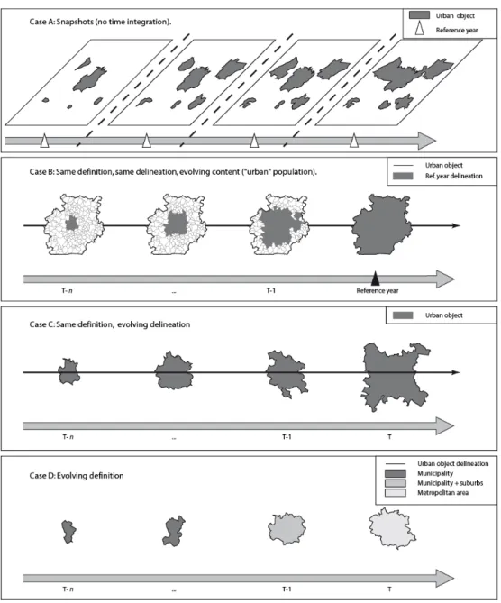
1. Choice of an evolving delineation for European urban areas Integrating time in urban databases depends first on a theoretical choice. Four different conceptual data models can be used for following urban objects through time (Bretagnolle et al. 2015 and Figure II-2). The choice depends on time span and quality of statistical and geometrical sources. For the TRADEVE project, we chose case B of Figure II-2, i.e. a

reconstruction of past delineations on the basis of present-day criteria. We applied the

same definition of urban areas through time (continuous built-up area, defined from Corine Land cover image and Urban Morphological Zones 2000), the same delineation (UMZ 2000) and an evolving content based on two different selection criteria applied to building blocks

12

(contiguity + constant minimum population threshold). When considered at different dates, these criteria enable the urban sprawl of a city to be followed by aggregating the surrounding villages that fulfill conditions at each date. This method has been applied from 1961 to 2001. For 2011, it was not possible to use the new UMZ built from Corine Land cover 2012 as population density grid which was used to build the dictionary of correspondence with LAU2 has not been updated since 2000. The 2011 LAU2 populations were then attributed to the 2000 perimeter.

Figure II-2 : Four models of time-integration in urban databases

Source: Bretagnolle et al. 2015

2. Criteria and parameters for selecting urban building blocks Two different criteria can be chosen in order to select urban building block at each date between 1961 and 2001: minimal density and minimal population. Both has been used

13

according to historical period or geographical region. For instance, the MUAs (Christian Vandermotten et al. 1999) are based on a minimal density threshold whereas the Geopolis database (Moriconi-Ebrard 1994) is based on a 200m distance and a minimal population threshold. We have then compared both methods and different parameters for each one (Annex C and D). We have finally chosen the minimal population methods and the 2000

threshold (discussion is presented in Section C.2).

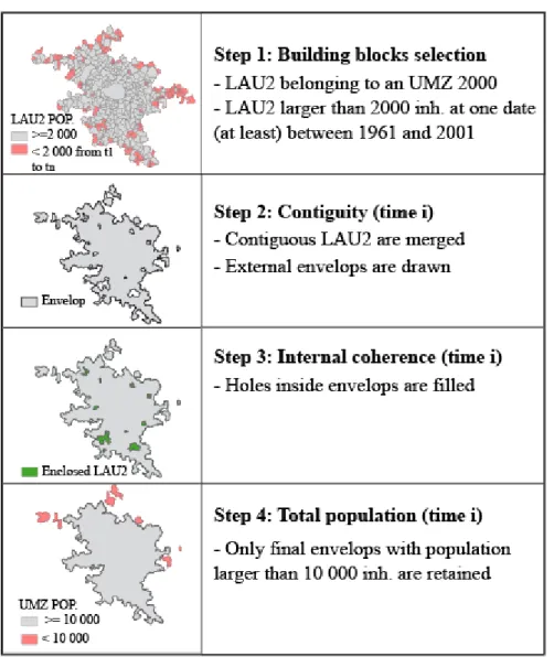
3. Construction of the task model

Four different steps2 were followed in order to apply the different criteria for the period 1961-2001. At the end of this operation, the UMZ 2000 are themselves reconstructed by the model. Consequently, their spatial coverage and total number are not the same than initially (Figure II-3).

2 _{In the Historical Population database (Gloersen et al. 2013), populations were attributed to LAU1 for} 4 different countries: Greece, Portugal, Lithuania and Slovenia (see II.A.2). For Greece and Slovenia, data were disaggregated at the LAU2 level by Gloersen et al. For Portugal and Lithuania, we used particular adaptations of LAU2 shapes (see II.A.3).

14

Figure II-3 : Four steps for constructing Tradeve urban areas

N-B: LAU2 are used for 25 countries and LAU1 for Greece, Portugal, Lithuania and Slovenia.

4. The resulting data model

The urban agglomerations that have been constructed in the TRADEVE project result from several databases (i.e. different statistical and geometrical sources), different types of relations (contiguity, administrative status at different levels of observation, etc.) and different parameters (thresholds, total figures etc.). A data model has been constructed in order to clarify the links between elements and the way they are evolving through time. This data-model is multi-level and dynamic (Figure II-4).

15

Figure II-4 : The TRADEVE data model

C. Methodological implementation 1. Presentation of the tools

We have used R© and Postgis in order to implement the methods described in the previous section. A new Postgis database has fist to be created (without any content), with a name and a password. The script Rpostgis is then used for uploading this Postgis database in R. At the beginning of the script, we indicate the path to the shape database and different parameters (see below). Information written in green color has to be fulfilled by the user.

Then the user indicated in the program the selection criteria (for instance, the 2000 inhabitants threshold).

16

Other criteria can be chosen by the user, for instance a density threshold (see below). In that case, the density variables have to be previously calculated.

In both cases population and density data have to be declared (for instance here: f2001pop, f1991pop, etc. ou f2001dens, f1991dens, etc.).

The next section of the program is dedicated to spatial processing. UMZ codes, LAU2 codes and population variables have to be declared (see below).

The last information that needs to be completed concerns the connection to the Postgis database.

17

The program is then executed. All the data are registered in the Postgis database and can be

easily and quickly accessed from Qgis by connecting Postgis and Qgis (see below).

This connection follows different steps described below.

2. Rational choice of the 2000 inh. minimal threshold

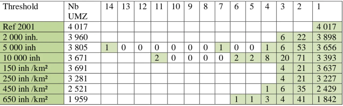
Results obtained for density and population are presented in Annex C and D (surface and population of LAU2 and Tradeve-UMZ). Tableau II-2 shows the total number of UMZ reconstructed for the year 2001.

18

Tableau II-2 : Total number of Tradeve-UMZ reconstructed for 2001 year according to different criteria and parameters

Threshold Nb UMZ 14 13 12 11 10 9 8 7 6 5 4 3 2 1 Ref 2001 4 017 4 017 2 000 inh. 3 960 6 22 3 898 5 000 inh 3 805 1 0 0 0 0 0 0 1 0 0 1 6 53 3 656 10 000 inh 3 671 2 0 0 0 0 2 2 8 20 71 3 393 150 inh /km² 3 691 4 21 3 637 250 inh /km² 3 281 4 21 3 227 450 inh /km² 2 521 1 6 35 2 429 650 inh /km² 1 959 1 1 3 4 41 1 842

The most restrictive thresholds lead to a more intense fragmentation of UMZ regarding the 2001 reference situation. Consequently, choosing the 2000 inh. or the 150 inh./km2 seems to be more appropriate.

Tableau II-3 shows the total number of Tradeve-UMZ according to the different criteria and parameters for each date.

Tableau II-3 : Total number of Tradeve-UMZ per year according to different criteria and parameters Seuil 2001 1991 1981 1971 1961 Abs. Rel. 2 000 inh 3 953 98,6% 3 877 3 775 3 548 3 248 5 000 inh 3 805 94,7% 3 699 3 571 3 345 3 044 10 000 inh 3 671 91,4% 3 593 3 491 3 284 2 995 150 inh /km² 3 691 91,9% 3 590 3 425 3 135 2 783 250 inh /km² 3 281 81,7% 3 135 2 946 2 648 2 265 450 inh /km² 2 521 62,8% 2 363 2 196 1 904 1 599 650 inh /km² 1 959 48,8% 1 837 1 708 1 480 1 200

Population thresholds better fit with the reference number of UMZ in 2001. For instance, when choosing the same density threshold than in the MUA database, i.e. 650 inh/km2, (Vandermotten et al. 1999), only 49% of the 2001 reference UMZ are kept. When choosing the 150 inh./km2 recommanded by OECE and used in several countries in Eastern Europe, the total number of reconstructed UMZ in 2001 is roughly the same than the one with the 10 000 inh. threshold. More specifically, the density threshold tends to reduce spatial coverage for countries characterized by large administrative units, and conversely tends to improve spatial coverage for countries with small units.

These different results favor the choice of the 2000 inh. population threshold. Validating the resulting database by comparison with other national or European databases confirm the relevance of this criteria.

19

D. Database validation

1. Spatial illustrations of evolving delineations

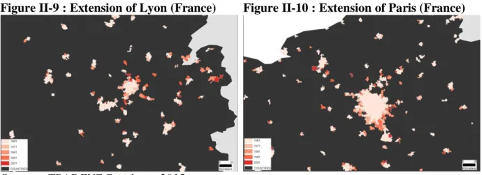
In North-Western Europe, large metropolises have known a major urban sprawl, with a spatial extent of suburbs and outer rings. Even if urban areas are not the most appropriate objects to capture peri-urbanisation, as they do not take into account commuting data, the methodology used in the TRADEVE project allows to follow the growth of some suburbs, for instance in western Denmark (Figure II-5), around Copenhagen (Figure II-6), Madrid (Figure II-7), Barcelona (Figure II-8), Paris (Figure II-10) or Lyon (Figure II-9). It confirms that measuring urban population and surface with evolving perimeters is most appropriate than considering a static delineation of urban areas.

Figure II-5 : Extension of urban areas in Jutland (Denmark)

Figure II-6 : Extension of urban areas in Eastern Denmark (including Copenhagen)

Sources: TRADEVE Database, 2015

Figure II-7 : Extension of Madrid (Spain) Figure II-8 : Extension of Barcelona (Spain)

20

Figure II-9 : Extension of Lyon (France) Figure II-10 : Extension of Paris (France)

Sources: TRADEVE Database, 2015

In Central Europe, such spatial extensions are less frequent, for two different reasons. First, urban sprawl due to automobile and rapid trains is more recent. Moreover, urban sprawl that began in the end of the 19th century throughout the construction of suburban railways was followed by successive annexations of surrounding LAU2 by the central municipality. Consequently, the size of the eponymous LAU2 (for instance Prague, or Budapest) was progressively enlarged, absorbing the new suburbs (see Prague on the Figure below, for instance). However, the Tradeve database allows to follow the rise of some new urban areas, as illustrated for instance in the north and east of Czech Republic (Figure II-11).

Figure II-11 : Extension of urban areas in Czech republic

Sources: TRADEVE Database, 2015

2. Statistical comparisons at national scale

We first compared the resulting Tradeve-UMZ and the French urban areas defined by national census board (INSEE) and named “unités urbaines” (Figure II-12).

21

For year 2000, we obtain 385 Tradeve UMZ and 455 Unités urbaines (1999 ref. year), covering respectively 30 606 km² and 51 302 km². Total urban population is 33 949 190 inh. and 37 321 923 inh. Only 2 Tradeve-UMZ are not corresponding to an Unité urbaine (Belleville, in the north of Lyon and Givet near the Belgium border). Conversely, 78 Unités urbaines do not correspond to a Tradeve-UMZ but are rather small (71 have a population lower than 15 000 inh. and 7 are between 15 000 and 25 000 inh.). In conclusion, the Tradeve-UMZ are less fragmented than the Unités urbaines (and consequently their total number is lower), which is easily understandable taking into account the method used by INSEE for constructing urban areas in France3.

When measuring indicators at a macro-level, such as an inequality index (slope in absolute value of a rank-size graph), results are very similar (Figure II-12 and Tableau II-4).

Figure II-12 : Rank-size graphs of French TRADEVE-UMZ and Unités urbaines

Tableau II-4 : Index of inequality sizes (absolute value of rank-size graph’s slope)

Tradeve-UMZ French Unités urbaines

1961/1962 1.03 0.98 1968/1971 1.06 1.03 1981/1982 1.06 1.05 1990/1991 1.06 1.06 1999/2001 1.06 1.06 2010/2011 1.05 1.07 3

This method is described in : « Composition communale des unités urbaines, Population et délimitation 1999, Nomenclatures et codes » ; INSEE, mars 1999. This is a method of construction of multi-commune “agglomerations” that is adapted to the fine scale of its LAU2. Morphological patches are first defined using the continuous built-up areas definitions, with the maximum distance between buildings of 200 meters (“zones bâties”). Then only LAU2 with more than 50% of their population laying in these “zones bâties” are retained in the urban area. Consequently, some of these building blocks may be very small, with a total population much lower than 2000 inhabitants.

y = 6E+06x-1,056 R² = 0,9904 10000 100000 1000000 10000000 1 10 100 1000 Population Rang

Tradeve-UMZ 2001 France

R² = 0,9932 10000 100000 1000000 10000000 1 10 100 1000 Population Rang

Unités Urbaines 1999

22

We also compared the resulting rank-size graphs for other European countries characterized by urban area definition based on continuous built-up areas: in 2001, in United-Kingdom we obtain 1.08 for Tradeve and 1.06 for national census, in Sweden we obtain 0,84 for Tradeve (but a R2=0.947) and 0.88 for national census. Results are rather similar.

3. Statistical comparisons at European scale

We used Geopolis database (Moriconi-Ebrard 1994) updated by Chatel 2012) for our comparisons (Tableau II-5 and Figure III-11).

Tableau II-5 : Comparison between Tradeve-UMZ and Geopolis database (total number and inequality index)

2011 2001 1991 1981 1971 1961

R² Slope R² Slope R² Slope R² Slope R² Slope R² Slope Rank-size Tradeve 0,992 0,94 0,991 0,94 0,991 0,948 0,992 0,951 0,994 0,954 0,996 0,945 Total number Tradeve 3 946 3 953 3 877 3 775 3 548 3 249 Rank-size Geopolis

R² Slope R² Slope R² Slope R² Slope R² Slope R² Slope 0.962*

Total number Geopolis

5426** 5453 5257 4942 4492

NB: The slope is presented in absolute value. Geopolis figures come from Chatel 2012. * This value was calculated including Turkey and Russia (Chatel, 2012, p. 503)

** (Chatel, 2012, p. 444)

III. Explorations of the resulting UMZ-T

database at the

European scale

In section III, IV and V, we explore some results of the UMZ-Tradeve database. As detailed in section II, this database is based on evolving urban perimeters.

A. Urbanization levels

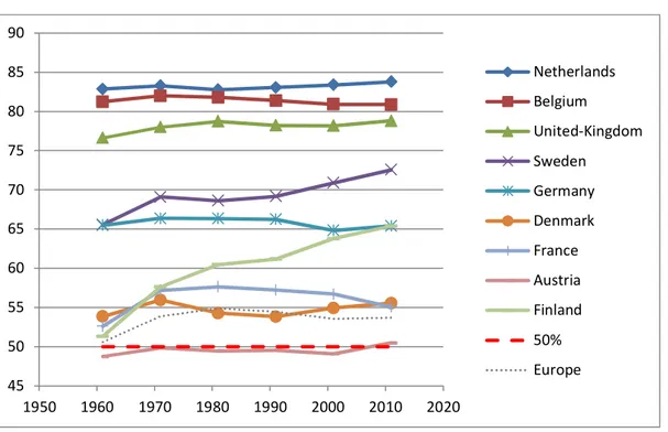
Luxembourg, Slovenia, Cyprus, Malta and Lichtenstein were removed, due to the weak number of UMZ. Plotting results for the 24 countries remaining on a same diagram would have given unreadable results. We decided to separate countries according to geographical criteria: those located in North-Western Europe, Atlantic and Mediterranean periphery and Central Europe.

1. North-Western Europe

All of these countries are in majority urban (urbanization level larger than 50%). However, urban dynamics are quite different. We observe a stagnation or even decline, for Germany, France and Belgium, probably due to the small perimeter of urban agglomerations that does not take into account commuting and peri-urbanization (Figure III-1). Austria seems to be very peripheral, as it is in reality if we consider its geographical position (she doesn’t belong

23

to north-western part of Europe). Urbanization level is growing in Nordic countries (Sweden and Finland).

Figure III-1 : Urbanization levels in North-Western Europe

2. Atlantic and Mediterranean periphery

We observe urban growth from 1961, stagnation after 1981/1991 except for Portugal, Greece and Finland (Figure III-2). In Ireland, demographic growth since 2001 is registered out of urban areas larger than 10 000 inh. (in rural or small settlements? Around large urban areas ?).

Figure III-2 : Urbanization levels in Atlantic and Mediterranean countries

45 50 55 60 65 70 75 80 85 90 1950 1960 1970 1980 1990 2000 2010 2020 Netherlands Belgium United-Kingdom Sweden Germany Denmark France Austria Finland 50% Europe 30 35 40 45 50 55 60 65 70 75 1950 1960 1970 1980 1990 2000 2010 2020 Italy Spain Greece Portugal Ireland 50% Europe

24

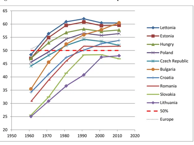
3. Central Europe

We observe a strong urban growth since 1961 then stagnation from 1991/2001, except for Bulgaria (total population decline) and Croatia (same) (Figure III-3).

Figure III-3 : Urbanization levels in Central Europe

B. Urban growth4

When mapped with circles proportional to their population (Figure III-4), using Tradeve-UMZ database, one can observe at each of the date the presence of the big metropolises of the European Megalopolis but also major large metropolises in the rest of Europe. Nevertheless urban growth has been even more remarkable in the Eastern part of Europe (Greece, socialist urban areas of Central and Eastern Europe with the exception of the Baltic ones) and in the Spanish coast. On the other side the last 20 years reveal a general tendency towards stagnation of this growth even though Paris, the most populated urban area has progressively reached a population above 10 000 000 inhabitants in this period (9 463 377 inhabitants in 1991 and 10 416 084 in 2011).

4 _{This section presents basic results obtained from a simple cartographic exploration of growth rates.} More sophisticated data processing is currently in progress in the framework of the ERC Geodivercity (Denise Pumain, Robin Cura et al.). For instance we question Gibrat model hypothesis (statistical independence between growth rates through time, statistical independence between growth rates and city sizes). Results should be published in 2016 or 2017.

20 25 30 35 40 45 50 55 60 65 1950 1960 1970 1980 1990 2000 2010 2020 Lettonia Estonia Hungry Poland Czech Republic Bulgaria Croatia Romania Slovakia Lithuania 50% Europe

25

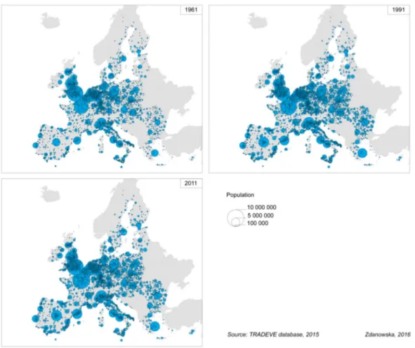
Figure III-4 : Population of urban areas in Europe (1961-2011, Tradeve-UMZ)

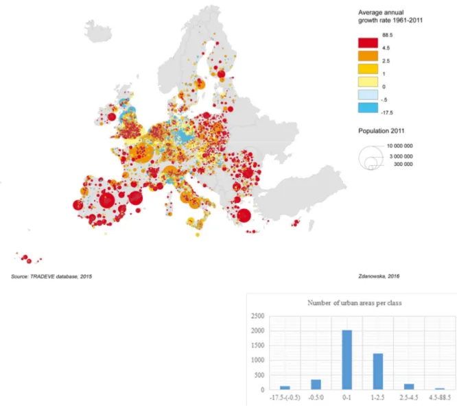
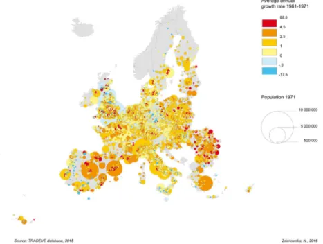
We also mapped average annual growth between 1961 and 2011 (Figure III-5). As the statistical distribution is highly dissymmetric (see the diagram below Figure III-5), we used a geometric progression in order to set the limits of the different classes. The map reveals that the majority of European urban areas have experienced positive urban growth in the last 50 years with the exception of German urban areas in the West and the East of the country, of urban areas in Northern Italy, Southern Hungary and the North of Great Britain (England and Scotland). Urban areas in Spain, Poland, Slovakia, Romania, Bulgaria and Greece have reached extremely highly annual growth rates (from 4.5 up to 88.5 percent) between 1961 and 2011. Medium size and small urban areas have also experienced important annual growth rates as it is the case of urban areas in France, in the Netherlands, in Southern England and Ireland.

26

Figure III-5 : Average annual growth rate of Tradeve-UMZ (1961 to 2011)

Table III-1 gives the evolution of the average annual growth rate for each period. Results show a progressive fall of growth between 1971 and 2001, with a recovery after 2001. We represented this evolution on 5 different maps (see below).

Table III-1: Average annual growth rate of European urban areas (Tradeve-UMZ) Period 1961-1971 1971-1981 1981-1991 1991-2001 2001-2011

European average annual growth rate (%)

0,014 0,008 0,004 0,002 0,004

In order to facilitate comparisons between the different periods, we used the same class limits for the 1961-2011 urban growth than for every decade inside this period. Urban annual growth of European urban areas has been mainly positive in the whole Europe (between 0 and 1 percent) in the period 1961-1971 (Figure III-6). However we can already point out at that time the decline of the population of urban areas in the Northern Europe (for example in large

27

urban areas of Great Britain) and a higher urban growth comparing to other urban areas in Spain, Greece and especially in Romania and Bulgaria.

Figure III-6 : Average annual growth rate of European urban areas between 1961 and 1971

In the period 1971-1981 (Figure III-7), the gap in terms of growth tendencies between Northern Europe and the other European countries has started to deepen. Indeed urban growth rates in Great Britain, Netherlands, Germany or Denmark have fallen comparing to the previous period to less than -0.5 percent. At the same time urban growth rates in Central and Eastern Europe and Spain have increased up to 4.5 percent or even more in the case of smaller urban areas of these regions.

28

Figure III-7 : Average annual growth rate of European urban areas between 1971 and 1981

The decade between 1981 and 1991 (Figure III-8) reveals a spread of negative urban growth throughout France, Northern Italy up to Rome and in a few large urban areas in Spain and Portugal (Barcelona and Lisbon). In addition, a decline of growth has taken place in very small urban areas of southern Hungary and in small sized urban areas in Bulgaria. Nevertheless in other Central Eastern European urban areas, the average annual growth rates have remained highly positive (especially in Romania).

29

Figure III-8 : Average annual growth rate of European urban areas between 1981 and 1991

Since 1991 (Figure III-9), Europe has passed through an equilibrations of urban growth rates and the tendencies have taken an opposite direction comparing to the previous period. Indeed Central and Eastern European urban areas have experienced slightly negative growth rates due to the spread of suburbanization. The growth rates in Western Europe have switched to slightly above zero (between 0 and 1 percent, and between 1 and 2.5 percent in the case of London). Moreover, urban areas with highest average urban growth rates have become exceptions (suburbs of Madrid, Barcelona, Paris, Athens and Klaipeda in Lithuania).

Figure III-9 : Average annual growth rate of European urban areas between 1991 and 2001

30

The beginning of the 21st century (Figure III-10) is marked by a certain recovery of urban growth in a few regions of Europe presenting average annual growth rates just above zero. It is the case of the whole United Kingdom, Central and Southern France, Belgium, the Netherlands, Denmark, Spain, Italy and Poland. Nevertheless, many urban areas in Germany, Hungary, Romania, Lithuania and Latvia have been still losing population as their annual growth rates were between -0.5 and -17.5 percent. An interesting point is that German central-eastern urban areas have never reached positive annual growth rates throughout the whole period 1961-2011, which confirms results from Figure III-4.

Figure III-10 : Average annual growth rate of Tradeve-UMZ (2001-2011)

C. Urban hierarchy

Rank-size graphs may be used for measuring urban concentration, when the regularity of the distribution of city size makes it possible to adjust the relationship between rank and urban population by way of a mathematical function. The slope of the adjustment, in absolute value, is an indicator of the degree of inequality of size among urban areas. When this degree increases over time, it means that the larger urban areas have a higher growth than average, leading to an urban concentration (or hierarchization).

Computed at the European level, the degree of inequality first increases, then declines during 30 years before increasing again (Figure III-11). We must however notice that these evolutions are very slight, the index oscillating between 0.94 and 0.95 for a period representing half a century. It means that the inequalities between city sizes are in fact very steady along this period.

31

Figure III-11 : Degree of inequality of urban area sizes in Europe, Tradeve-UMZ (1961-2011)

Only countries with a determination coefficient R2>= 0.96 at each date have been retained: Slovakia, Sweden, Greece, Ireland and the Netherlands were removed, also Hungry and Latvia in 1961, Portugal before 2001. Luxembourg, Slovenia, Cyprus, Malta, Estonia, Lithuania and Lichtenstein were removed, due to the weak number of UMZ.

In North-Western, Atlantic and Mediterranean Europe, urban concentration is rather high (Figure III-12), which can be explained by two different reasons. First, urban transition began in the 19th century and large urban areas have registered a relative growth higher than the average one since this period. Secondly, in some countries like Belgium, Netherlands or some regions in United-Kingdom, large conurbations are very frequent. For instance in Belgium, Brussels UMZ has a population of 4,38 million inhabitants as it includes Anvers. We can also notice that the urban concentration is generally decreasing, probably because the outer rings populated with commuters are not taken into account in the Tradeve definition of urban areas. With functional urban areas, it would be different and large entities would probably continue to register a higher growth than the average.

0,938 0,940 0,942 0,944 0,946 0,948 0,950 0,952 0,954 0,956 1950 1960 1970 1980 1990 2000 2010 2020

Europe

32

Figure III-12 : Degree of inequality in urban area sizes, North-Western, Atlantic and Mediterranean Europe

In Central Europe, urban concentration is generally growing then decreasing, except for Bulgaria and Romania where it is still increasing (Figure III-13).

Figure III-13 : Degree of inequality in urban area sizes, Central Europe

0,80 0,90 1,00 1,10 1,20 1,30 1,40 1,50 1950 1960 1970 1980 1990 2000 2010 2020 Belgium United-Kingdom Austria Spain France Italy Germany Finlande Portugal Europe 0,700 0,800 0,900 1,000 1,100 1,200 1,300 1950 1960 1970 1980 1990 2000 2010 2020 Europe Bulgaria Croatia Poland Czech Republic Romania Slovakia Hungry Latvia

33

D. Urban trajectories

The harmonized database Tradeve-UMZ is a useful tool to carry out comparative approach at the European level. Using the same morphological definition of urban areas allows us to perform some reliable statistical classifications. In this part we report the main outcomes of a hierarchical cluster analysis performed on demographic trajectories (between 1961 and 2011)

of 3962 Tradeve-UMZ5.

In order to conduct these data explorations, we applied the Ward method (which tends to minimize intra-class variance and to maximize inter-class variance) on a matrix (using Chi-2 distance), which was resulting of a correspondence analysis on the temporal population table. This methodology is convenient because it highlights the urban trajectory similarities and it understates stock effects.

Figure III-14: Hierarchical cluster analysis on trajectories of Trdeve-UMZ (1961-2011)

5

In order to avoid blanks in the database, we had to remove 20 small UMZ that had merged into larger agglomerations during the period 1961-2011 to execute the hierarchical cluster analysis.

34

We can identify four main clusters6 (Figure III-14). More than 60% of European UMZs show

an urban trajectory similar to Clusters 1 and 2: a certain growth of population during the whole period with a slight slowdown since 1991. Clusters 3 and 4 describe interesting trends. “Cluster 3” (representing more than 20% of all the UMZs) aggregates stagnation and decay profiles and includes some large urban areas (explaining the high value of the mean). “Cluster 4” is the smaller one (only 330 UMZs) and it shows a strong population growth profile. Taking a look at the clusters relative weight (Figure III-15) reveals that “Cluster 4” is a very specific one, concerning an important share of small and medium sized urban areas.

Figure III-15: Relative weight of the four clusters

Following this first exploration, we provide three cartographic representations of the previous clustering.

This first map (Figure III-16) shows Tradeve-UMZ envelops and the cluster typology. This kind of representation is useful to see trends in highly urbanized areas such as Belgium, Germany and Netherlands for example.

6

We have set up the hierarchical cluster analysis in 4 clusters using both dendrogram (Figure III-14) and bar plots about inertia explained (Annex VIII.F). Bar plots indicate that it is relevant to choose 3 or 4 nodes (meaning 4 or 5 clusters), but the dendrogram shows that Cluster 1 will be divided if we choose 5 clusters, bringing no relevant profile.

35

Figure III-16: Demographic trajectories of Tradeve-UMZ (1961-2011), urban surfaces

The second representation (Figure III-17) doesn’t take into account size and population of urban areas. It is convenient to identify spatial patterns and sizes of the four clusters. We can clearly see the East/West opposition with an important demographic dynamism for the eastern countries (Poland/ Czech Republic/ Romania/ Bulgaria) and a relative strong decay/stagnation patterns on former industrial western countries (Germany/ Northern Italy/ Eastern France). We can also identify a higher concentration of “Cluster 4 UMZs” (strong growth) located on the Mediterranean coastline (reflecting the “littoralization” process).

36

Figure III-17: Demographic trajectories of Tradeve-UMZ (1961-2011), urban patterns

The third representation (Figure III-18) is a classic one. We have used proportional circles to show size effects of demographic trajectories. We can identify the same patterns than with Figure III-17, but in addition we clearly see a North/South opposition with a strong decay/stagnation pattern in the Northern Europe (partly due to the aging population). Furthermore, we can notice that most of Cluster 4 small urban areas (strong demographic growth profiles) are located around large urban areas, reflecting some “metropolization“ processes in Western Europe.

37

Figure III-18: Demographic trajectories of Tradeve-UMZ (1961-2011), urban populations

Tableau III-1 and Tableau III-2 give the results by country. Red boxes indicate an overrepresentation of UMZ of clusters 3 or 4 (> Global mean + 0,5 Sd) and yellow boxes indicate an under-representation of UMZs of clusters 3 or 4 (< Global mean – 0,5 Sd). Apart from pointing out very small countries, these tables confirm some trends that we have seen on maps: for example, demographical trends of Irish and Spanish UMZs reflecting a more general population growth in these countries, and also the strong pattern of decay and stagnation for German UMZs.

38

Tableau III-1: Hierarchical Cluster Analysis outcomes by country (count)

Clusters Country 1 2 3 4 Total AT 11 22 18 1 52 BE 4 29 14 47 BG 42 10 17 69 CH 1 1 CY 5 5 CZ 44 48 13 1 106 DE 174 295 287 12 768 DK 18 15 11 4 48 EE 8 1 3 1 13 ES 150 52 22 76 300 FI 10 21 9 2 42 FR 123 104 114 33 374 GR 24 17 4 6 51 HR 20 6 3 3 32 HU 28 31 37 3 99 IE 12 3 10 25 IT 126 239 131 22 518 LT 7 2 3 12 LU 3 3 LV 13 1 7 1 22 MT 1 1 NL 87 57 16 20 180 PL 170 86 14 32 302 PT 22 24 13 5 64 RO 94 25 9 21 149 SE 12 36 29 6 83 SI 4 3 1 8 SK 42 3 1 19 65 UK 197 156 94 44 491 Total 1442 1288 870 330 3930

39

Tableau III-2: Hierarchical Cluster Analysis outcomes by country (share in percent)

IV. Urban trajectories at national level for selected countries

Hierarchical cluster analysis performed at the European level can be compared to results obtained at a national scale. We selected here a few examples.

A. Germany

In Germany, we can observe in the clustering at the European level an overrepresentation of “Cluster 3 UMZs” grouping both stagnation and decay profiles (Figure IV-1). The hierarchical cluster analysis performed at the national level only shows a more precise representation with three clusters: decay trends in blue (Cluster 3), stagnation trends in yellow (Cluster 1), light population growth in orange (Cluster 2). Figure IV-2 enlightens the East/West opposition with an obvious decay pattern for urban areas located in Saxony. It also appears that the only growing agglomerations are small and medium sized urban areas located around metropolitan regions and attesting a polycentric urban development.

Clusters Country 1 2 3 4 Total AT 21,2 42,3 34,6 1,9 1,3 BE 8,5 61,7 29,8 0,0 1,2 BG 60,9 14,5 24,6 0,0 1,8 CH 0,0 0,0 100,0 0,0 0,0 CY 0,0 0,0 0,0 100,0 0,1 CZ 41,5 45,3 12,3 0,9 2,7 DE 22,7 38,4 37,4 1,6 19,5 DK 37,5 31,3 22,9 8,3 1,2 EE 61,5 7,7 23,1 7,7 0,3 ES 50,0 17,3 7,3 25,3 7,6 FI 23,8 50,0 21,4 4,8 1,1 FR 32,9 27,8 30,5 8,8 9,5 GR 47,1 33,3 7,8 11,8 1,3 HR 62,5 18,8 9,4 9,4 0,8 HU 28,3 31,3 37,4 3,0 2,5 IE 48,0 12,0 0,0 40,0 0,6 IT 24,3 46,1 25,3 4,2 13,2 LT 58,3 0,0 16,7 25,0 0,3 LU 0,0 100,0 0,0 0,0 0,1 LV 59,1 4,5 31,8 4,5 0,6 MT 0,0 100,0 0,0 0,0 0,0 NL 48,3 31,7 8,9 11,1 4,6 PL 56,3 28,5 4,6 10,6 7,7 PT 34,4 37,5 20,3 7,8 1,6 RO 63,1 16,8 6,0 14,1 3,8 SE 14,5 43,4 34,9 7,2 2,1 SI 50,0 37,5 12,5 0,0 0,2 SK 64,6 4,6 1,5 29,2 1,7 UK 40,1 31,8 19,1 9,0 12,5 Total 36,7 32,8 22,1 8,4 100,0

40

Figure IV-1: Demographic trajectories of German urban areas (1961-2011) (Hierarchical Cluster Analysis at the European level)

Figure IV-2: Demographic trajectories of German urban areas (1961-2011) (Hierarchical Cluster Analysis at the national level)

41

B. Romania

Comparison between the two kinds of classification is very useful to understand Romanian demographic trends. Indeed, the hierarchical cluster analysis at the European scale (Figure IV-3) provides a good summary of growth trends between 1961 and 1991 but it does not adequately take “post-1990 situations” into account. Figure IV-4 presents a more accurate representation of recent demographic trends. We can see that since 1991 and later when the Soviet Union dissolved, urban growth just stopped and a phase of decay started (there are several explanation to this phenomenon, particularly the combination of two factors: a strong emigration to Western Europe and a lower birth rate).

Figure IV-3: Demographic trajectories of Romanian urban areas (1961-2011) (Hierarchical Cluster Analysis at the European level)

Figure IV-4: Demographic trajectories of Romanian urban areas (1961-2011) (Hierarchical Cluster Analysis at the national level)

42

C. Spain

Spanish demographic trends show a general population growth pattern. Both clustering at European and Spanish levels present the same trends: a stable population growth during the whole period with a light slowdown in the past decade (Figure IV-5 and Figure IV-6). The latter figure shows that slowing population growth mainly concerns large urban areas. We can also identify urban sprawl patterns around large metropolitan agglomerations because small urban areas next to larger ones are experiencing the strongest growth.

Figure IV-5: Demographic trajectories of Spanish urban areas (1961-2011) (Hierarchical Cluster Analysis at the European level)

Figure IV-6: Demographic trajectories of Spanish urban areas (1961-2011) (Hierarchical Cluster Analysis at the national level)

43

D. United Kingdom

Figure IV-7 and Figure IV-8 almost enlighten the same urban dynamics. The latter shows that “Cluster 1” (in blue) represents a light decay of population between 1971 and 1991, and a very light regrowth since that date. This trend concerns the large urban areas and it reveals two different things: in the London’s case it means that urban growth takes place in outer suburbs and not in the core city, whereas in the North it represents some consequences of the deindustrialization processes.

Figure IV-7: Demographic trajectories of British urban areas (1961-2011) (Hierarchical Cluster Analysis at the European level)

Figure IV-8: Demographic trajectories of British urban areas (1961-2011) (Hierarchical Cluster Analysis at the national level)

44

V.

Focus on Decay and Stagnation Patterns

As seen before, the hierarchical cluster analysis at the European level produces 4 clusters. “Cluster 3”, gathering stagnation and decay profiles, is particularly interesting (Figure III-14). In order to distinguish different trends, we selected the 883 urban areas that belong to this cluster and we carried out another hierarchical cluster analysis (using the same method)7. As result, there are 4 clusters, and we choose to remove one of them (“Cluster 4”) representing only two Italian urban areas8 (Figure V-1).

We can identify three main urban trajectories. “Cluster 1” (blue) represents actual decay trends during the whole period (1961-2011). Relative stagnation profiles, with some slow re-growth since 1991, are represented by “Cluster 2” (yellow). And finally, “Cluster 3” (rose) gathers urban areas that have known a certain population growth between 1961 and 1981, following by a phase of decay since 1981.

Figure V-1: Demographic trajectories and population 2011 of the European urban areas characterized by decay or stagnation (1961-2011)

7

For sure, we can achieve the same result by increasing the number of clusters in the first cluster analysis but it is less readable because dendrogram (Figure III-14) indicates that clusters 1 and 4 will be divided first.

8

45

VI. Conclusion

We described in this TRADEVE report the different steps that were followed for constructing a harmonized longitudinal database giving delineations and populations of urban areas at the European level (29 countries), from 1961 to 2011 (5 dates). These urban areas are defined by taking into account continuous build-up areas (from Urban Morphological Zones database, produced by EEA and enriched by ESPON Database 2008-2014) and minimal population threshold (2000 inhabitants for building blocks and 10 000 inhabitants for urban areas). Populations come from Historical Population Database (Gloersen et al 2013) with corrections from the TRADEVE project. Our methods give 3946 urban areas in 2011, and 3249 in 1961. We presented in section 2 the different methods that have been used for retropolating UMZ to 1961, by using and correcting for some countries and by populating the 2000 perimeter with 2011 data. In Section 3, we presented different explorations of the resulting database, at the European level, for urban growth, urban hierarchy and demographic trajectories. Section 4 presents results two Hierarchical Cluster Analysis (European level and national level) for a few selected countries: Germany, Spain, Romania and United-Kingdom.

These results are very promising and invite us to invest deeper in two different directions. First by expertizing results at national scale for other countries that those covered by the Tradeve experts, for instance in Scandinavia, Central Europe, Italy, Greece, Portugal, Netherlands etc. Of course, Tradeve-UMZ database does not pretend to replace national databases, that are based on a long historical tradition of census boards and researchers expertize, but to give another point of view, based on a top-down definition applied in the same way in all European countries (at least those for which we have UMZ and Population density grid data). Some people may think that results tend to minimize urbanization process in some countries (for instance in Slovenia), due to the high minimal population level (10 000 inhabitants), but we assume that one of the main interests of Tradeve-UMZ are precisely to give another point of view, in order to complete (and not replace) the national one.

The second direction will consist to invest construction of Functional Urban Areas around Tradeve-UMZ by using methods proposed in ESPON Database 2008-2014 and based on accessibility isochrones (including speed parameters) (see Guérois et al. 2014 and 2016). We are fully aware that working on European urban areas implies to take into account functional perimeters and not only perimeters based on continuous built-up areas. This is a real challenge and we hope that Tradeve-UMZ will be associated in the future to functional urban areas designed around them. But we also want to recall the importance and interest of urban areas database, that allow to work on small entities: if the majority of European inhabitants live in urban areas (58% according to Tradeve-UMZ database in 2001), nearly half live in medium and small size ones, populated by less than 50 000 inhabitants.

46

VII. References

Bretagnolle A., Delisle F., Mathian H., Vatin G. (2015), « Urbanization of the United States over two centuries: an approach based on a long-term database (1790-2010)”, in International Journal of Geographical Information Science, vol. 29, issue 15, pp. 850-857.

Bretagnolle A., Guérois M., Le Nechet F., Mathian H., Pavard A. (2016), « La ville à l’échelle de l’Europe : Apports du couplage et de l’expertise de bases de données issues de l’imagerie satellitale », Revue Internationale de Géomatique.

Bretagnolle A., Guérois M., Mathian H., Pavard A. (2014), UMZ: a data base now operational for urban studies (M4D improvements). Technical report, 30 June 2014,

downloadable from ESPON Database website

http://database.espon.eu/db2/resource?idCat=31, 33 pages.

Cheshire P. (1995), A new phase of urban development in western Europe? The evidence for the 1980s’. Urban Studies 32(7):1045–1063.

Dijkstra L., Poelman H. (2012), Cities in Europe. The new OECD-EC definition. Regional Focus, RF 01/2012, Regional and Urban Policy, 15 pages.

Gallego F. J. (2010), A Population density grid of the European Union, Population and Environment, vol. 31, n°6, pp. 460-473.

Gloersen E., Lüer C. (2013), Population Data Collection for European Local Administrative Units from 1960 onward. Final Report – Data are available on Eurostat’s website:

http://ec.europa.eu/eurostat/web/nuts/local-administrative-units

Guérois M., Bretagnolle A., Giraud T., Mathian H. (2012), "A new database for the cities of Europe? Urban Morphological Zones (CLC2000) confronted to three national databases of urban agglomerations (Denmark, France Sweden)", Environment and Planning B, vol. 39 (3), pages 439-458.

Guérois M., Bretagnolle A., Mathian H., Pavard A. (2014), Functional Urban Areas (FUA) and European harmonization : A feasibility study from the comparison of two approaches: commuting flows and accessibility isochrones. Technical report, 30 June 2014, downloadable

from ESPON Database website http://database.espon.eu/db2/resource?idCat=31, 36 pages.

Guérois M., Bretagnolle A., Mathian H., Pavard A. (2016, accepted), « Les temps de transport pour délimiter des aires urbaines fonctionnelles ? Une investigation critique à partir de trois métropoles européennes », Belgeo, Revue Belge de Géographie, to be published in 2016. Milego R. (2007), Urban Morphological Zones, Definition and procedural steps, Report, Copenhagen: European Environment Agency, European Topic Centre Terrestrial Environment, 9 p.

47

Turok Ivan, Mykhnenko Vlad (2007), “The trajectories of European Cities, 1960-2005”, in Cities, vol. 24 n°3, pp.165-182.

Vandermotten Christian, Vermoesen Frank, De Lannoy Walter, De Corte Stefan (1999), « Villes d’Europe. Cartographie comparative », in Bulletin du Crédit Communal, Trimestriel, 53ème année, n°207-208, 407 pages.

VIII. Annexes

A. Historical Population Database: Computing specifications per country

Group 1 Group 2 Group 3

Interpolation realized by National census boards

Interpolation realized by Foresight team Using other limits

than EBM 2012 Austria Belgium Croatia * Estonia Finland France Hungry Lichtenstein Luxembourg Macedonia * Norway Sweden Netherlands Serbia * Bulgaria Cyprus Czech Republic

Germany (according to landers) Island Malta Romania Slovakia Spain Specificities

Italy : data population

for 1961-91 have been recalculated according to 1991 limits. For 2000-11, limits are 2012 ones. An estimation has been produced by for the

whole period by

covering 1991 units with 2012 ones.

North Ireland: Data are available in a grid

format 1km/1km for 1971-2001. Previous data are available according to the 1851 electoral divisions.

Poland: geolocation in 1975 limits of the

1960 and 1970

demographic data. For the following years,

minimizing bias

induced by limits

variations by creating specific base maps.

Ireland Republic: Fusion of LAU2

(electoral districts) for certain dates due to statistical secret (national census have to diffuse aggregated data for some districts). Data for 1961, 71 and 81 are diffused in different geometries. An estimation has been realized by associating residential address and recent limits.

Portugal: high variation of LAU2 limits

through time and large number of unitsà LAU1 units.

Lithuania: LAU1

data, but not in a

vector format à

digitalization of the limits.

Slovenia: 1994 reform lead to LAU2

48

been kept and gave LAU1 à LAU1 units.

Denmark: Territorial reform in 2007 (the

276 LAU2 were divided into 2116 parishes). LAU2 populations for years prior to 2007 have been calculated from a spatial interpolation between new LAU2 and parishes (point data).

United-Kingdom:

high number of local limit changes.

Greece : Data prior to 1991 were not

available in a numeric format. Base map that has been used is a national one.

Leetonia and Romania: Territorial reform

that lead to LAU2 divisions. For prior dates: aggregation of LAU2.

* All the demographic data for Serbia, Croatia and Macedonia after 1990 are contested. ** Kosovo is not classified in one of the 3 groups. No specific information.

B. Data Checking of the Historical Population database, per country

Autriche

Méthode Interpolation des données pour obtenir les données au 1er janvier

1961 / 1971 / 1981 / 1991 / 2001.

Les données ont été calculées dans le découpage géographique de 2012. Particularité du RP De Jure *** Dates Recensements 01/06/1951 21/03/1961 12/05/1971 12/05/1081 15/05/1991 15/05/2001 Calculs effectués par Statistika Austria

Droit d’utilisation Diffusion autorisée. Utilisation à des fins commerciales interdites.

Mention de la source obligatoire : Source: Population censuses 1951-2001 (Volkszählungen 1951 bis 2001).

Unités dans la base harmonisée

2357

Identifiées par le code commune Statistika Austria. Couche LAU2 2001 Couche LAU2 2008 Couche LAU2 2010 2359 2358 2357

Données nationales Populations communales 1869 à 2001.

Données récupérées sur le site de l’ONS

Dans les délimitations 2001. Harmonisées aux délimitations 2012. Vérif data rétropolées

Eurostat ü

Vérification d’absence de valeurs adhérentes (croisement des populations observées et populations calculées). Exemple : Création d’un