HAL Id: hal-01807468
https://hal.archives-ouvertes.fr/hal-01807468
Submitted on 13 Nov 2020
HAL is a multi-disciplinary open access
archive for the deposit and dissemination of
sci-entific research documents, whether they are
pub-lished or not. The documents may come from
teaching and research institutions in France or
abroad, or from public or private research centers.
L’archive ouverte pluridisciplinaire HAL, est
destinée au dépôt et à la diffusion de documents
scientifiques de niveau recherche, publiés ou non,
émanant des établissements d’enseignement et de
recherche français ou étrangers, des laboratoires
publics ou privés.
The Sloan Digital Sky Survey Quasar Catalog:
Fourteenth data release
Isabelle Pâris, Patrick Petitjean, Éric Aubourg, Adam D. Myers, Alina
Streblyanska, Brad W. Lyke, Scott F. Anderson, Éric Armengaud, Julian
Bautista, Michael R. Blanton, et al.
To cite this version:
Isabelle Pâris, Patrick Petitjean, Éric Aubourg, Adam D. Myers, Alina Streblyanska, et al.. The Sloan
Digital Sky Survey Quasar Catalog: Fourteenth data release. Astron.Astrophys., 2018, 613, pp.A51.
�10.1051/0004-6361/201732445�. �hal-01807468�
Astronomy
&
Astrophysics
https://doi.org/10.1051/0004-6361/201732445
© ESO 2018
The Sloan Digital Sky Survey Quasar Catalog:
Fourteenth data release
?
Isabelle Pâris
1, Patrick Petitjean
2, Éric Aubourg
3, Adam D. Myers
4, Alina Streblyanska
5,6, Brad W. Lyke
4,
Scott F. Anderson
7, Éric Armengaud
8, Julian Bautista
9, Michael R. Blanton
10, Michael Blomqvist
1,
Jonathan Brinkmann
11, Joel R. Brownstein
9, William Nielsen Brandt
12,13,14, Étienne Burtin
8, Kyle Dawson
9,
Sylvain de la Torre
1, Antonis Georgakakis
15, Héctor Gil-Marín
16,17, Paul J. Green
18, Patrick B. Hall
19,
Jean-Paul Kneib
20, Stephanie M. LaMassa
21, Jean-Marc Le Goff
8, Chelsea MacLeod
18, Vivek Mariappan
9,
Ian D. McGreer
22, Andrea Merloni
15, Pasquier Noterdaeme
2, Nathalie Palanque-Delabrouille
8,
Will J. Percival
23, Ashley J. Ross
24, Graziano Rossi
25, Donald P. Schneider
12,13, Hee-Jong Seo
26,
Rita Tojeiro
27, Benjamin A. Weaver
28, Anne-Marie Weijmans
27, Christophe Yèche
8,
Pauline Zarrouk
8, and Gong-Bo Zhao
29,23 (Affiliations can be found after the references) Received 10 December 2017 / Accepted 14 January 2018ABSTRACT
We present the data release 14 Quasar catalog (DR14Q) from the extended Baryon Oscillation Spectroscopic Survey (eBOSS) of the Sloan Digital Sky Survey IV (SDSS-IV). This catalog includes all SDSS-IV/eBOSS objects that were spectroscopically targeted as quasar candidates and that are confirmed as quasars via a new automated procedure combined with a partial visual inspection of spectra, have luminosities Mi[z= 2] < −20.5 (in a ΛCDM cosmology with H0 = 70 km s−1Mpc−1,ΩM= 0.3, and ΩΛ= 0.7), and
either display at least one emission line with a full width at half maximum larger than 500 km s−1or, if not, have interesting/complex
absorption features. The catalog also includes previously spectroscopically-confirmed quasars from SDSS-I, II, and III. The catalog contains 526 356 quasars (144 046 are new discoveries since the beginning of SDSS-IV) detected over 9376 deg2(2044 deg2having new
spectroscopic data available) with robust identification and redshift measured by a combination of principal component eigenspectra. The catalog is estimated to have about 0.5% contamination. Redshifts are provided for the MgIIemission line. The catalog identifies 21 877 broad absorption line quasars and lists their characteristics. For each object, the catalog presents five-band (u, g, r, i, z) CCD-based photometry with typical accuracy of 0.03 mag. The catalog also contains X-ray, ultraviolet, near-infrared, and radio emission properties of the quasars, when available, from other large-area surveys. The calibrated digital spectra, covering the wavelength region 3610–10 140 Å at a spectral resolution in the range 1300 < R < 2500, can be retrieved from the SDSS Science Archiver Server.
Key words. catalogs – surveys – quasars: general
1. Introduction
Since the identification of the first quasar redshift bySchmidt
(1963), each generation of spectroscopic surveys has enlarged
the number of known quasars by roughly an order of magnitude:
the Bright Quasar Survey (Schmidt & Green 1983) reached the
100 discoveries milestone, followed by the Large Bright Quasar
Survey (LBQS; Hewett et al. 1995) and its 1000 objects, then the
∼25 000 quasars from the 2dF Quasar Redshift Survey (2QZ; Croom et al. 2004), and the Sloan Digital Sky Survey (SDSS; York et al. 2000) with over 100 000 new quasars (Schneider et al.
2010). Many other surveys have also significantly contributed
to increase the number of known quasars (e.g.Osmer & Smith
1980;Boyle et al. 1988;Storrie-Lombardi et al. 1996).
Each iteration of SDSS has pursued different science goals, and hence set different requirements for their associated quasar target selection.
SDSS-I/II (York et al. 2000) aimed to observe ∼105quasars;
The final quasar list was presented in the SDSS data release 7
?http://www.sdss.org/dr14/algorithms/qso_catalog
(DR7) quasar catalog (Schneider et al. 2010). The main science
driver was studies of the quasar population through the
measure-ment of their luminosity function (e.g. Richards et al. 2006)
and clustering properties (e.g. Hennawi et al. 2006;Shen et al.
2007). The quasar program of SDSS-I/II also led to the
discov-ery of a significant sample of z > 5 quasars (e.g. Fan et al. 2006; Jiang et al. 2008), large samples of broad absorption line (BAL)
quasars (e.g. Reichard et al. 2003; Trump et al. 2006;Gibson
et al. 2008), type 2 candidates (Reyes et al. 2008) or samples of objects with peculiar properties such as weak emission lines (Diamond-Stanic et al. 2009). Quasar target selection algorithms
for SDSS-I/II are fully detailed in Richards et al. (2002) and
Schneider et al.(2010).
The main motivation to observe quasars with
SDSS-III/BOSS (Eisenstein et al. 2011; Dawson et al. 2013) was to
constrain the Baryon Acoustic Oscillation (BAO) scale at z ∼ 2.5
using the HI located in the intergalactic medium (IGM) as a
tracer of large scale structures. About 270 000 quasars, mostly in the redshift range 2.15–3.5 for which at least part of the Lyman-α forest lies in the spectral range, have been discovered by SDSS-III/BOSS. The measurement of the auto-correlation
A51, page 1 of17
function of the Lyman-α forest (e.g. Bautista et al. 2017) and the cross-correlation of quasars and the Lyman-α forest (e.g. du Mas des Bourboux et al. 2017) have provided unprecedented cosmological constraints at z ∼ 2.5. This sample was also used
to study the luminosity function of quasars (Ross et al. 2013;
Palanque-Delabrouille et al. 2013), moderate-scale clustering of
z ∼ 2.5 quasars (e.g. Eftekharzadeh et al. 2015). Repeat
spec-troscopic observations of BAL quasars have been performed to
constrain the scale and dynamics of quasar outflows (Filiz Ak
et al. 2012, 2013, 2014). Peculiar population of quasars have been also identified in this enormous sample such as z > 2
type 2 quasar candidates (Alexandroff et al. 2013) or extremely
red quasars (Ross et al. 2015; Hamann et al. 2017). In order
to maximize the number of z > 2 quasars, the target selection for SDSS-III/BOSS used a variety of target selection algorithms (Bovy et al. 2011, 2012; Kirkpatrick et al. 2011; Yèche et al. 2010; Palanque-Delabrouille et al. 2011;Richards et al. 2004).
The overall quasar target selection strategy is described inRoss
et al.(2012).
Quasar observation in SDSS-IV is driven by multiple scien-tific goals such as cosmology, understanding the physical nature of X-ray sources and variable sources.
SDSS-IV/eBOSS aims to constrain the angular-diameter
dis-tance dA(z) and the Hubble parameter H (z) in the redshift range
0.6–3.5 using four different tracers of the underlying density
field over 7500 deg2: 250 000 new luminous red galaxies (LRG)
at 0.6 < z < 1.0, 195 000 new emission line galaxies (ELG) at 0.7 < z < 1.1, 450 000 new quasars at 0.9 < z < 2.2, and the Lyman-α forest of 60 000 new z > 2.2 quasars.
SDSS-IV/SPIDERS (SPectroscopic IDentification of
ERosita Sources) investigates the nature of X-ray emitting
sources, including active galactic nuclei (Dwelly et al. 2017)
and galaxy clusters (Clerc et al. 2016). Initially, SPIDERS
targets X-ray sources detected mainly in the ROSAT All Sky
Survey (Voges et al. 1999, 2000) which has recently been
reprocessed (Boller et al. 2016). In late 2018, SPIDERS plans to
begin targeting sources from the eROSITA instrument on board
the Spectrum Roentgen Gamma satellite (Predehl et al. 2010;
Merloni et al. 2012). About 5% of eBOSS fibers are allocated to SPIDERS targets. A total of 22 000 spectra of active galactic nuclei are expected by the end of the survey, about 5000 of them being also targeted by SDSS-IV/eBOSS.
Finally, SDSS-IV/TDSS (Time Domain Spectroscopic Sur-vey) that aims to characterize the physical nature of time-variable sources, primarily on sources detected to be variable in
Pan-STARRS1 data (PS1; Kaiser et al. 2010) or between SDSS
and PS1 imaging, has been allocated about 5% of eBOSS fibers (Morganson et al. 2015; MacLeod et al. 2017). The targets identified in PS1 are a mix of quasars (about 60%) and stel-lar variables (about 40%). It will lead to the observation of about 120 000 quasars with a majority of them also targeted by SDSS-IV/eBOSS.
This paper presents the SDSS-IV/eBOSS quasar cata-log, denoted DR14Q, that compiles all the spectroscopically-confirmed quasars identified in the course of any of the SDSS iterations and released as part of the SDSS
Four-teenth data release (Abolfathi et al. 2017). The bulk of the
newly discovered quasars contained in DR14Q arise from the
main SDSS-IV/eBOSS quasar target selection (Myers et al.
2015). The rest were observed by ancillary programs (83 430
quasars not targeted by the SDSS-IV/eBOSS main quasar
survey; see Dawson et al. 2013; Ahn et al. 2014; Alam
et al. 2015), and TDSS and SPIDERS (27 547 and 1090, respectively).
We summarize the target selection and observations in
Sect.2. We describe the visual inspection process and describe
the definition of the DR14Q parent sample in Sect.3. We discuss
the accuracy of redshift estimates in Sect.4and present our
auto-mated detection of BAL quasars in Sect.5. General properties of
the DR14Q sample are reviewed in Sects.6and7, and the
for-mat of the catalog is described in Sect.8. Finally, we conclude
in Sect.9.
In the following, we use a ΛCDM cosmology with H0
= 70 km s−1Mpc−1, ΩM = 0.3, Ω
Λ = 0.7 (Spergel et al.
2003). We define a quasar as an object with a luminosity
Mi[z= 2] < −20.5 and either displaying at least one emission
line with a full-width at half maximum (FWHM) > 500 km s−1
or, if not, having interesting/complex absorption features. Indeed, a few tens of objects have weak emission lines but the
Lyman-α forest is clearly visible in their spectra (
Diamond-Stanic et al. 2009), and thus they are included in the DR14Q catalog. About 200 quasars with unusual BALs are also included
in our catalog (Hall et al. 2002) even though they do not
formally meet the requirement on emission-line width. All mag-nitudes quoted here are point spread function (PSF) magmag-nitudes (Stoughton et al. 2002) and are corrected for Galactic extinction (Schlafly & Finkbeiner 2011).
2. Survey outline
In this section, we focus on imaging data used to perform the target selection of SDSS-IV quasar programs and new spectro-scopic data obtained since August 2014.
2.1. Imaging data
Three sources of imaging data have been used to target quasars in
SDSS-IV/eBOSS (full details can be found inMyers et al. 2015):
updated calibrations of SDSS imaging, the Wide-Field Infrared
Survey (WISE; Wright et al. 2010), and the Palomar Transient
Factory (PTF; Rau et al. 2009;Law et al. 2009).
SDSS imaging data were gathered using the 2.5 m wide-field
Sloan telescope (Gunn et al. 2006) to collect light for a camera
with 30 2k × 2k CCDs (Gunn et al. 1998) over five broad bands
– ugriz (Fukugita et al. 1996). A total of 14 555 unique square
degrees of the sky were imaged by this camera, including
con-tiguous areas of ∼7500 deg2 in the North Galactic Cap (NGC)
and ∼3100 deg2in the SGC that comprise the uniform “Legacy”
areas of the SDSS (Aihara et al. 2011). These data were acquired
on dark photometric nights of good seeing (Hogg et al. 2001).
Objects were detected and their properties were measured by the photometric pipeline (Lupton et al. 2001;Stoughton et al. 2002) and calibrated photometrically (Smith et al. 2002;Ivezi´c et al. 2004;Tucker et al. 2006;Padmanabhan et al. 2008), and
astro-metrically (Pier et al. 2003). Targeting for eBOSS is conducted
using SDSS imaging that is calibrated to theSchlafly et al.(2012)
Pan-STARRS solution (Finkbeiner et al. 2016). These imaging
data were publicly released as part of SDSS-DR13 (Albareti et al.
2016).
The quasar target selection for SDSS-IV/eBOSS also makes use of the W1 and W2 WISE bands centered on 3.4 and 4.6 µm. The “unWISE” coadded photometry is applied to sources
detected in the SDSS imaging data as described inLang(2014).
This approach produces photometry of custom coadds of the WISE imaging at the position of all SDSS primary sources.
Imaging data from PTF is also used to target quasars using variability in SDSS-IV/eBOSS. Starting from the individual
calibrated frames available from IPAC (Infrared Processing &
Analysis Center; Laher et al. 2014), a customized pipeline is
applied to build coadded PTF images on a timescale adapted to quasar targeting, i.e. typically 1–4 epochs per year, depending on the cadence and total exposure time within each field. A stack of all PTF imaging epochs is also constructed to create a catalog of PTF sources. Finally, light curves are created using coadded PTF images to perform the selection of quasar candidates.
2.2. Target selection
In order to achieve a precision of 2.8% on dA(z) and 4.2% on
H(z) measurement with the quasar sample, it is necessary to
achieve a surface density of at least 58 quasars with 0.9 < z < 2.2
per square degree (Dawson et al. 2016). The SDSS-IV/eBOSS
“CORE” sample is intended to recover sufficient quasars in this specific redshift range and additional quasars at z > 2.2 to sup-plement SDSS-III/BOSS. The CORE sample homogeneously targets quasars at all redshifts z > 0.9 based on the XDQSOz
method (Bovy et al. 2012) in the optical and a WISE-optical
color cut. To be selected, it is required that point sources have a XDQSOz probability to be a z > 0.9 quasar larger than 0.2
and pass the color cut mopt− mWISE ≥(g − i) + 3, where mopt
is a weighted stacked magnitude in the g, r and i bands and
mWISEis a weighted stacked magnitude in the W1 and W2 bands.
Quasar candidates have g < 22 or r < 22 with a surface density
of confirmed new quasars (at any redshifts) of ∼70 deg−2.
SDSS-IV/eBOSS also selects quasar candidates over a wide range of redshifts using their photometric variability measured from the PTF. In the following we refer to this sample as the “PTF” sample. These targets have r > 19 and g < 22.5 and provide an additional 3–4 z > 2.1 quasars per deg2.
In addition, known quasars with low quality SDSS-III/BOSS spectra (0.75 < S /N per pixel < 3)1 or with bad spectra are re-observed.
Finally, quasars within 100 of a radio detection in the FIRST
point source catalog (Becker et al. 1995) are targeted.
A fully detailed description of the quasar target selection in SDSS-IV/eBOSS and a discussion of its performance can be found inMyers et al.(2015).
TDSS targets point sources that are selected to be variable
in the g, r and i bands using the SDSS-DR9 imaging data (Ahn
et al. 2012) and the multi-epoch Pan-STARRS1 (PS1) photome-try (Kaiser et al. 2002,2010). The survey does not specifically target quasars in general but a significant fraction of targets
belong to this class (Morganson et al. 2015). Furthermore, there
are smaller sub-programs (comprising 10% of the main TDSS
survey) that target quasars specifically (MacLeod et al. 2017).
Therefore, these quasars are included in the parent sample for the quasar catalog.
Finally, the AGN component of SPIDERS targets X-ray sources detected in the concatenation of the Bright and Faint
ROSAT All Sky Survey (RASS) catalogs (Voges et al. 1999,
2000) and that have an optical counterpart detected in the DR9
imaging data (Ahn et al. 2012). Objects with 17 < r < 22 that lie
within 10of a RASS source are targeted. Details about the AGN
target selection are available inDwelly et al.(2017). 2.3. Spectroscopy
Spectroscopic data for SDSS-IV are acquired in a similar
man-ner as for SDSS-III (Dawson et al. 2016). Targets identified by
1 This measurement refers to the standard SDSS spectroscopic
sam-pling of 69 km s−1per pixel.
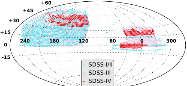
Fig. 1.Distribution on the sky of the SDSS-DR14/eBOSS spectroscopy in J2000 equatorial coordinates (expressed in decimal degrees). Cyan dots correspond to the 1462 plates observed as part of SDSS-I/II. The purple area indicates the 2587 plates observed as part of SDSS-III/BOSS. The red area represents to the 496 new plates observed as part of SDSS-IV (i.e. with MJD ≥ 56 898).
the various selection algorithms are observed with the BOSS spectrographs whose resolution varies from ∼1300 at 3600 Å to
2500 at 10 000 Å (Smee et al. 2013). Spectroscopic
observa-tions are obtained in a series of at least three 15-min exposures. Additional exposures are taken until the squared signal-to-noise
ratio (S/N)2 per pixel reaches the survey-quality threshold for
each CCD. These thresholds are (S /N)2 ≥ 22 at i-band
magni-tude for the red camera and (S /N)2 ≥ 10 at g-band magnitude
for the blue camera (Galactic extinction-corrected magnitudes). The spectroscopic reduction pipeline for the BOSS spectra is
described inBolton et al.(2012). SDSS-IV uses plates covered
by 1000 fibers that have a field of view of approximately 7 deg2. The plates are tiled in a manner which allows them to overlap (Dawson et al. 2016). Figure1shows the locations of observed plates. The total area covered by the DR 14 of SDSS-IV/eBOSS
is 2044 deg2. Figure2presents the number of spectroscopically
confirmed quasars with respect to their observation date.
3. Construction of the DR14Q catalog
Unlike the SDSS-III/BOSS quasar catalogs (Pâris et al. 2012,
2014,2017), the SDSS-IV quasar catalog also contains all the
quasars observed as part of SDSS-I/II/III. This decision is driven by one of the scientific goals of SDSS-IV/eBOSS to use quasars
as the tracers of large scale structures at z ∼ 1.5 (see Dawson
et al. 2016;Blanton et al. 2017): quasars observed as part of the first two iterations of SDSS with a high-quality spectrum, i.e. a spectrum from which one can measure a redshift, were not
re-observed as part of SDSS-IV (see Myers et al. 2015, for further
details).
3.1. Definition of the superset
The ultimate goal of the SDSS quasar catalog is to gather all the quasars observed as part of any of the stages of SDSS (York et al. 2000;Eisenstein et al. 2011;Blanton et al. 2017). To do so, we need to create a list of quasar targets as complete as possible that we refer to as the superset. Its definition for the DR14Q catalog depends on the iteration of the SDSS during which a quasar was observed:
– SDSS-I/II: we use the list of confirmed quasars in the SDSS-DR7 quasar catalog that contains all
spectroscopi-cally confirmed quasars from SDSS-I/II (Schneider et al.
2010). A total of 79 487 quasars with no re-observation in
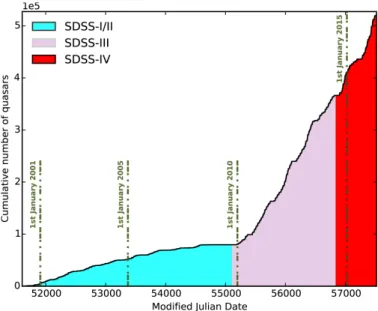
Fig. 2. Cumulative number of quasars as a function of observation date during all the iterations of SDSS (York et al. 2000;Eisenstein et al. 2011;
Blanton et al. 2017). Vertical lines show the equivalence between mod-ified Julian dates and usual calendar dates. A total of 526 356 quasars have been spectroscopically confirmed. The “flat portions” in this figure correspond to annual summer shutdown for the telescope maintenance.
– SDSS-III/IV: we follow the definition of the superset as in Pâris et al.(2017). Our input list of quasar targets is com-posed of all quasar targets as defined by their target selection bits. The full list of programs targeting quasars and associ-ated references is given in Table1. This set contains objects targeted as part of the legacy programs but also all the ancil-lary programs that targeted quasars for specific projects (see e.g. Dawson et al. 2013, for examples of ancillary pro-grams). A total of 819 611 quasar targets are identified using target selection bits described in Table1.
The superset we obtain contains 899 098 objects to be classified. 3.2. Automated classification
Given the increase of the number of quasar targets in IV, the systematic visual inspection we performed in SDSS-III/BOSS (e.g. Pâris et al. 2012) is no longer feasible. Since the
output of the SDSS pipeline (Bolton et al. 2012) cannot be fully
efficient to classify quasar targets, we adopt an alternate strategy: starting from the output of the SDSS pipeline, we identify SDSS-IV quasar targets for which it is likely the identification and redshifts are inaccurate. This set of objects is visually inspected
following the procedure described in Sect.3.3.
The spectra of quasar candidates are reduced by the SDSS
pipeline2, which provides a classification (QSO, STAR or GALAXY)
and a redshift. This task is accomplished using a library of stellar templates and a principal component analysis (PCA) decomposition of galaxy and quasar spectra are fitted to each spectrum. Each class of templates is fitted in a given range
of redshift: galaxies from z = −0.01 to 1.00, quasars from
z = 0.0033 to 7.00, and stars from z = −0.004 to 0.004
(±1200 km s−1). For each spectrum, the fits are ordered by
increasing reduced χ2; the overall best fit is the fit with the lowest reduced χ2.
2 The software used to reduce SDSS data is called idlspec2d. Its DR14
version is v5_10_0.
We start with the first five identifications, i.e.
identifica-tions corresponding to the five lowest reduced χ2, redshifts and
ZWARNING. The latter is a quality flag. Whenever it is set to 0, its classification and redshift are considered reliable. We then apply the following algorithm:
1. if the first SDSS pipeline identification is STAR, then the resulting classification is STAR;
2. if the first SDSS pipeline identification is GALAXY with zpipeline< 1, then the resulting classification is GALAXY; 3 if the first SDSS pipeline identification is GALAXY with
zpipeline ≤ 1 and at least two other SDSS pipeline
iden-tifications are GALAXY, then the resulting classification is GALAXY;
4. if the first SDSS pipeline identification is QSO with ZWARNING = 0, then the resulting classification is QSO, except if at least two other SDSS pipeline identifications are STAR. In such a case, the resulting identification is STAR;
5. if the first pipeline identification is QSO with ZWARNING > 0 and at least two alternate SDSS pipeline identifications are STAR, then the resulting identification is STAR.
At this stage, the redshift measurement we consider for automat-ically classified objects is the redshift estimate of the overall best fit of the SDSS pipeline, except if the automated identification is STAR. In that case, we set the redshift to 0. If an object does not pass any of these conditions, the resulting classification is UNKNOWN and it is added to the list of objects that require visual inspection (see Sect.3.3).
In order to achieve the expected precision on the dA(z) and
H(z) measurements, it is required (i) to have <1% of actual
quasars lost in the classification process and (ii) to have <1% of contaminants in the quasar catalog. We tested this algorithm against the result of the full visual inspection of the “SEQUELS” pilot survey of SDSS-IV/eBOSS that contains a total of 36 489 objects (see Myers et al. 2015;Pâris et al. 2017, for details) to ensure that these requirements are fulfilled.
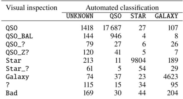
Out of these 36 489 objects, 2393 (6.6% of the whole sam-ple) cannot be classified by the automated procedure, 18 799 are classified as QSO, 10 001 as STAR, and 5288 as GALAXY. For objects identified as QSO by the algorithm, 98 are wrongly classified. This represents a contamination of the quasar sam-ple of 0.5%. A total of 158 actual quasars, i.e. identified in the course of the full visual inspection, are lost which represents 0.8% of the whole quasar sample. The latter number includes 12 objects identified as QSO_Z? by visual inspection because their identification is not ambiguous. Detailed results for the com-parison with the fully visually inspected sample are provided in Table2.
The performance of this algorithm depends on the SDSS pipeline version and the overall data quality. To ensure that this performance does not change significantly, we fully visu-ally inspect randomly picked plates regularly and test the quality of the output.
3.3. Visual inspection process
Depending on the iteration of SDSS, different visual inspection strategies have been applied.
3.3.1. Systematic visual inspection of SDSS-III quasar candidates
As described in Pâris et al. (2012), we visually inspected all
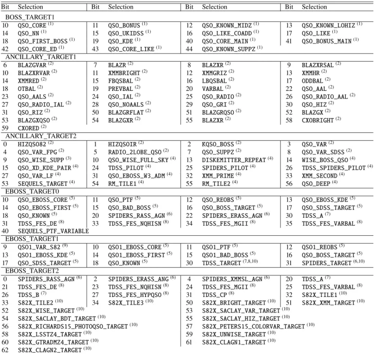
Table 1. Programs from SDSS-III/BOSS (Eisenstein et al. 2011;Dawson et al. 2013) and SDSS-IV (Dawson et al. 2016;Blanton et al. 2017) targeting quasars and taken as inputs to build up the SDSS-DR14 quasar catalog.
Bit Selection Bit Selection Bit Selection Bit Selection
BOSS_TARGET1
10 QSO_CORE(1) 11 QSO_BONUS(1) 12 QSO_KNOWN_MIDZ(1) 13 QSO_KNOWN_LOHIZ(1)
14 QSO_NN(1) 15 QSO_UKIDSS(1) 16 QSO_LIKE_COADD(1) 17 QSO_LIKE(1) 18 QSO_FIRST_BOSS(1) 19 QSO_KDE(1) 40 QSO_CORE_MAIN(1) 41 QSO_BONUS_MAIN(1)
42 QSO_CORE_ED(1) 43 QSO_CORE_LIKE(1) 44 QSO_KNOWN_SUPPZ(1)
ANCILLARY_TARGET1
6 BLAZGVAR(2) 7 BLAZR(2) 8 BLAZXR(2) 9 BLAZXRSAL(2)
10 BLAZXRVAR(2) 11 XMMBRIGHT(2) 12 XMMGRIZ(2) 13 XMMHR(2)
14 XMMRED(2) 15 FBQSBAL(2) 16 LBQSBAL(2) 17 ODDBAL(2)
18 OTBAL(2) 19 PREVBAL(2) 20 VARBAL(2) 22 QSO_AAL(2)
23 QSO_AALS(2) 24 QSO_IAL(2) 25 QSO_RADIO(2) 26 QSO_RADIO_AAL(2)
27 QSO_RADIO_IAL(2) 28 QSO_NOAALS(2) 29 QSO_GRI(2) 30 QSO_HIZ(2) 31 QSO_RIZ(2) 50 BLAZGRFLAT(2) 51 BLAZGRQSO(2) 52 BLAZGX(2) 53 BLAZGXQSO(2) 54 BLAZGXR(2) 55 BLAZXR(2) 58 CXOBRIGHT(2)
59 CXORED(2)
ANCILLARY_TARGET2
0 HIZQSO82(2) 1 HIZQSOIR(2) 2 KQSO_BOSS(2) 3 QSO_VAR(2)
4 QSO_VAR_FPG(2) 5 RADIO_2LOBE_QSO(2) 7 QSO_SUPPZ(2) 8 QSO_VAR_SDSS(2)
9 QSO_WISE_SUPP(3) 10 QSO_WISE_FULL_SKY(4) 13 DISKEMITTER_REPEAT(4) 14 WISE_BOSS_QSO(4)
15 QSO_XD_KDE_PAIR(4) 24 TDSS_PILOT(4) 25 SPIDERS_PILOT(4) 26 TDSS_SPIDERS_PILOT(4)
27 QSO_VAR_LF(4) 31 QSO_EBOSS_W3_ADM(4) 32 XMM_PRIME(4) 33 XMM_SECOND(4)
53 SEQUELS_TARGET(4) 54 RM_TILE1(4) 55 RM_TILE2(4) 56 QSO_DEEP(4) EBOSS_TARGET0
10 QSO_EBOSS_CORE(5) 11 QSO_PTF(5) 12 QSO_REOBS(5) 13 QSO_EBOSS_KDE(5) 14 QSO_EBOSS_FIRST(5) 15 QSO_BAD_BOSS(5) 16 QSO_BOSS_TARGET(5) 17 QSO_SDSS_TARGET(5)
18 QSO_KNOWN(5) 20 SPIDERS_RASS_AGN(6) 22 SPIDERS_ERASS_AGN(6) 30 TDSS_A(7)
31 TDSS_FES_DE(8) 33 TDSS_FES_NQHISN(8) 34 TDSS_FES_MGII(8) 35 TDSS_FES_VARBAL(8)
40 SEQUELS_PTF_VARIABLE EBOSS_TARGET1
9 QSO1_VAR_S82(9) 10 QSO1_EBOSS_CORE(5) 11 QSO1_PTF(5) 12 QSO1_REOBS(5) 13 QSO1_EBOSS_KDE(5) 14 QSO1_EBOSS_FIRST(5) 15 QSO1_BAD_BOSS(5) 16 QSO_BOSS_TARGET(5)
17 QSO_SDSS_TARGET(5) 18 QSO_KNOWN(5) 30 TDSS_TARGET(7,8,10) 31 SPIDERS_TARGET(6,10)
EBOSS_TARGET2
0 SPIDERS_RASS_AGN(6) 2 SPIDERS_ERASS_ANG(6) 4 SPIDERS_XMMSL_AGN(6) 20 TDSS_A(7)
21 TDSS_FES_DE(8) 23 TDSS_FES_NQHISN(8) 24 TDSS_FES_MGII(8) 25 TDSS_FES_VARBAL(8)
26 TDSS_B(7) 27 TDSS_FES_HYPQSO(8) 31 TDSS_CP(8) 32 S82X_TILE1(10)
33 S82X_TILE2(10) 34 S82X_TILE3(10) 50 S82X_BRIGHT_TARGET(10) 51 S82X_XMM_TARGET(10) 52 S82X_WISE_TARGET(10) 53 S82X_SACLAY_VAR_TARGET(10) 54 S82X_SACLAY_BDT_TARGET(10) 55 S82X_SACLAY_HIZ_TARGET(10) 56 S82X_RICHARDS15_PHOTOQSO_TARGET(10) 57 S82X_PETERS15_COLORVAR_TARGET(10) 58 S82X_LSSTZ4_TARGET(10) 59 S82X_UNWISE_TARGET(10) 60 S82X_GTRADMZ4_TARGET(10) 61 S82X_CLAGN1_TARGET(10) 62 S82X_CLAGN2_TARGET(10)
References.(1)Ross et al.(2012).(2)Dawson et al.(2013).(3)Ahn et al.(2014).(4)Alam et al.(2015).(5)Myers et al.(2015).(6)Dwelly et al.(2017). (7)Morganson et al.(2015).(8)MacLeod et al.(2017).(9)Palanque-Delabrouille et al.(2016).(10)Abolfathi et al.(2017).
2011;Dawson et al. 2013). The idea was to construct a quasar catalog as complete and pure as possible (this was also the approach adopted by SDSS-I/II catalogs). Several checks dur-ing the SDSS-III/BOSS survey have shown that completeness (within the given target selection) and purity are larger than 99.5%.
After their observation, all the spectra are automatically
clas-sified by the SDSS pipeline (Bolton et al. 2012). Spectra are
divided into four categories based on their initial classification by the SDSS pipeline: low-redshift quasars (i.e. z < 2), high-redshift quasars (i.e. z ≥ 2), stars and others. We perform the
visual inspection plate by plate through a dedicated website: all spectra for a given category can be validated at once if their identification and redshift are correct. If an object requires fur-ther inspection or a change in its redshift, we have the option to go to a detailed page on which not only the identification can be changed but also BALs and DLAs can be flagged and the
redshift can be adjusted. When possible the peak of the MgII
emission line was used as an estimator of the redshift (see Pâris
et al. 2012), otherwise the peak of CIV was taken as the indi-cator in case the redshift given by the pipeline was obviously in error.
Table 2. Comparison between the automated classification scheme based on the output of the SDSS pipeline (Bolton et al. 2012) and visual inspection of our training set.
Visual inspection Automated classification
UNKNOWN QSO STAR GALAXY
QSO 1418 17 687 27 107 QSO_BAL 144 946 4 8 QSO_? 79 27 6 26 QSO_Z? 120 41 5 7 Star 213 11 9804 189 Star_? 61 5 54 29 Galaxy 74 37 23 4623 ? 115 15 34 95 Bad 169 30 44 204
3.3.2. Residual visual inspection of SDSS-IV quasar candidates
For SDSS-IV/eBOSS, we visually inspect only the objects the automated procedure considers ill-identified. Most of the corre-sponding spectra are, unsurprisingly, of low S/N. A number of ill-identified sources have good S/N but show strong absorption lines which confuse the pipeline. These objects can be strong BALs but also spectra with a strong DLA at the emission redshift (Finley et al. 2013;Fathivavsari et al. 2017). A few objects have very unusual continua. The visual inspection itself proceeds as for the SDSS-III/BOSS survey. However, we no longer visually flag BALs and we change redshifts only in case of catastrophic failures of the SDSS pipeline.
3.4. Classification result
Starting from the 899 098 unique objects included in the DR14Q
superset, we run the automated procedure described in Sect.3.2.
A total of 42 729 quasar candidates are classified as UNKNOWN by the algorithm. Identification from the full visual inspection of SDSS-I/II/III quasar targets was already available for 625 432 objects, including 32 621 identified as UNKNOWN by the auto-mated procedure. The remaining 10 108 quasar candidates with no previous identification from SDSS-I/II/III have been visually inspected. After merging all the already existing identifications, 635 540 objects are identified through visual inspection and 263 558 are identified by the automated procedure.
A total of 526 356 quasars are identified, 387 223 from visual inspection and 139 133 from the automated classification.
Results are summarized in Table3.
4. Redshift estimate
Despite the presence of large and prominent emission lines, it is frequently difficult to estimate accurate redshifts for quasars. Indeed, the existence of quasar outflows create systematic shifts in the location of broad emission lines leading to not fully
con-trolled errors in the measurement of redshifts (e.g. Shen et al.
2016). Accuracy in this measurement is crucial to achieve the
scientific goals of SDSS-IV/eBOSS. As stated in the Sect. 5.2 ofDawson et al.(2016), we mitigate this problem by using two different types of redshift estimates: one based on the result of a principal component analysis and another one based on the
location of the maximum of the peak of the MgIIemission line.
4.1. Automated redshift estimates
Various studies have shown that the MgIIemission line is the
quasar broad emission line that is the least affected by systematic shifts (e.g. Hewett & Wild 2010;Shen et al. 2016). In the BOSS spectral range, this feature is available in the redshift range 0.3– 2.5, which covers most of our sample.
To measure the MgIIredshift (Z_MGII), we first perform a
principal component analysis (PCA) on a sample of 8986
SDSS-DR7 quasars (Schneider et al. 2010) using input redshifts from
Hewett & Wild(2010). The detailed selection of this sample is
explained in Sect. 4 of Pâris et al. (2012). With the resulting
set of eigenspectra, we fit a linear combination of five princi-pal components and measure the location of the maximum of
the MgIIemission line. This first step produces a new redshift
measurement that can be used to re-calibrate our reference sam-ple. We then perform another PCA with Z_MGII and derive a new set of principal components. In this second step it is not necessary to have Z_MGII but this step is mandatory to
derive PCA redshifts calibrated to use the MgIIemission as a
reference.
Finally, to measure Z_PCA, we fit a linear combination of four eigenspectra to all DR14Q spectra. The redshift estimate is an additional free parameter in the fit. During the fitting process, there is an iterative removal of absorption lines in order to limit
their impact on redshift measurements; Details are given inPâris
et al.(2012).
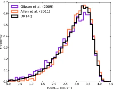
4.2. Comparison of redshift estimates provided in DR14Q In the present catalog, we release four redshift estimates: Z_PIPE, Z_VI, Z_PCA, and Z_MGII. As explained in the
pre-vious section, the MgIIemission line is the least affected broad
emission line in quasar spectra. In addition, this emission line is available for most of our sample. We use it as the reference red-shift to test the accuracy of our three other redred-shift estimates. For this test, we select all the DR14Q quasars for which we have the four redshift estimates. Among these 178 981 objects, we also select 151 701 CORE quasars only to test the behavior of our estimates on this sample for which redshift accuracy is cru-cial. Figure3displays the distribution of the velocity differences between Z_VI, Z_PIPE, Z_PCA and Z_MGII for the full sample having the four redshift estimates available (left panel) and CORE
quasars only (right panel). Table4gives the systematic shift for
each of the distributions and the dispersion of these quantities, expressed in km s−1, for both samples.
As explained in Sect.3.3, the visual inspection redshift Z_VI
is set to be at the location of the maximum of the MgII
emis-sion line when this line is available. With this strategy, the
systematic shift with respect to the MgIIemission line is
lim-ited by the accuracy of the visual inspection. Although it is a time-consuming approach, this redshift estimate produces an extremely low number of redshift failures (<0.5%), leading to a low dispersion around this systematic shift.
The SDSS pipeline redshift estimate, Z_PIPE, is the result of a principal component analysis performed on a sample of visually-inspected quasars. Hence, Z_PIPE is expected to have a similar systematic shift as Z_VI. On the other hand, Z_PIPE is subject to more redshift failures due to peculiar objects or low S/N spectra and thus the larger dispersion of the velocity difference distribution seen in Fig.3and Table4.
Z_PCA is also the result of a principal component analysis but, unlike Z_PIPE, the reference sample has been carefully cho-sen to have an automated redshift corresponding to the location
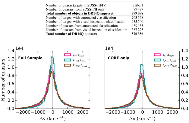
Table 3. Result of our classification process, split between automated and visual inspection classifications.
Number of quasar targets in SDSS-III/IV 819 611
Number of quasars from SDSS-I/II only 79 487
Total number of objects in DR14Q superset 899 098
Number of targets with automated classification 263 558
Number of targets with visual inspection classification 635 540
Number of quasars from automated classification 139 133
Number of quasars from visual inspection classification 387 223
Total number of DR14Q quasars 526 356
Fig. 3.Left panel: distribution of velocity differences between Z_VI (magenta histogram), Z_PIPE (brown histogram), Z_PCA (dark cyan histogram) and Z_MGII. These histograms are computed using 178 981 quasars that have all the four redshift estimates available in DR14Q. Right panel: same as left panel restricted to the 151 701 CORE quasars for which we have the four redshift estimates available in DR14Q. In both panels, the histograms are computed in bins of∆v = 50 km s−1and the vertical grey line marks∆v = 0 km s−1.
of the maximum of the MgIIemission line. Therefore, a
system-atic shift smaller than 10 km s−1was expected when compared
to Z_MGII. In addition, Z_PCA takes into account the possible presence of absorption lines, even broad ones, and it is trained to ignore them. Z_PCA is thus less sensitive to peculiarities in quasar spectra, which explains the reduced dispersion of redshift errors when compared to Z_PIPE.
A similar analysis performed on a sample of 151 701 CORE quasars for which we have the four redshift estimates leads to similar results for redshift estimates. These exercises demon-strate that there is no additional and significant systematics for the redshift estimate of the CORE quasar sample.
5. Broad absorption line quasars
In SDSS-III/BOSS, we performed a full visual inspection of all quasar targets. During this process, we visually flagged spectra displaying BALs. With this catalog, it is no longer possible to visually inspect all BALs and we now rely on a fully automated detection of BALs.
As for the previous SDSS quasar catalogs, we automatically search for BAL features and report metrics of common use in the
community: the BALnicity Index (BI; Weymann et al. 1991) of
the CIVabsorption troughs. We restrict the automatic search to
quasars with z ≥ 1.57 in order to have the full spectral coverage
of CIV absorption troughs. The BALnicity Index (Col. #32) is
Table 4. Median shift and dispersion of velocity differences between Z_VI, Z_PIPE, Z_PCA and Z_MGII for the full DR14Q sample and the CORE sample only.
Median∆v σ∆v
(km s−1) (km s−1)
Full sample (178 981 quasars)
zVI− zMgII −59.7 585.9
zPIPE− zMgII −54.8 697.2
zPCA− zMgII −8.8 586.9
CORE sample (151 701 quasars)
zVI− zMgII −61.7 581.0
zPIPE− zMgII −57.9 692.1
zPCA− zMgII −9.3 577.4
Notes. These numbers are derived from a subsample of 178 981 quasars from DR14Q for which we have the four redshift estimates available. We also restrict this analysis to 151 701 CORE quasars for which we also have the four different redshift estimates. See Fig.3for the full distributions.
computed bluewards of the CIVemission line and is defined as:
BI= − Z 3000 25 000 " 1 − f(v) 0.9 # C(v)dv, (1)
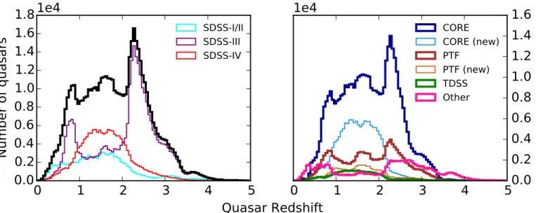
Fig. 4. Distribution of the logarithm of the CIVBALnicity Index for BAL quasars in DR14Q (black histogram), (Gibson et al. 2009, violet histogram) and (Allen et al. 2011, orange histogram). All the histograms are normalized to have their sum equal to one. Histograms have bin widths of log BICIV= 0.1.
where f (v) is the normalized flux density as a function of velocity displacement from the emission-line center. The quasar continuum is estimated using the linear combination of four
prin-cipal components as described in Sect. 4.1. C(v) is initially set
to 0 and can take only two values, 1 or 0. It is set to 1 when-ever the quantity 1 − f (v)/0.9 is continuously positive over an
interval of at least 2000 km s−1. It is reset to 0 whenever this
quantity becomes negative. CIVabsorption troughs wider than
2000 km s−1are detected in the spectra of 21 877 quasars.
The distribution of BI for CIVtroughs from DR14Q is
pre-sented in Fig.4(black histogram) and is compared to previous
works by Gibson et al.(2009, purple histogram) performed on
DR5Q (Schneider et al. 2007) and byAllen et al.(2011, orange
histogram) who searched for BAL quasars in quasar spectra
released as part of SDSS-DR6 (Adelman-McCarthy et al. 2008).
The three distributions are normalized to have their sum equal to one. The overall shapes of the three distributions are similar.
The BI distribution fromGibson et al.(2009) exhibits a slight
excess of low-BI values (log BICIV< 2) compared toAllen et al.
(2011) and this work. The most likely explanation is the
differ-ence in the quasar emission modeling.Allen et al. (2011) used
a non-negative matrix factorization (NMF) to estimate the unab-sorbed flux, which produces a quasar emission line shape akin to
the one we obtain with PCA.Gibson et al.(2009) modeled their
quasar continuum with a reddened power-law and strong emis-sion lines with Voigt profiles. Power-law like continua tend to underestimate the actual quasar emission and hence, the result-ing BI values tend to be lower than the one computed when the quasar emission is modeled with NMF or PCA methods.
6. Summary of the sample
The DR14Q catalog contains 526 356 unique quasars, of which 144 046 are new discoveries since the previous release. This dataset represents an increase of about 40% in the number of SDSS quasars since the beginning of SDSS-IV.
Spectro-scopic observations of quasars were performed over 9376 deg2
for SDSS-I/II/III. New SDSS-IV spectroscopic data are available over 2044 deg2. The average surface density of 0.9 < z < 2.2
quasars prior to the beginning of SDSS-IV is 13.27 deg−2, and
reaches 80.24 deg−2in regions for which SDSS-IV spectroscopy
is available. The overall quasar surface density in regions with
SDSS-IV spectroscopy is 125.03 deg−2, which corresponds to an
increase by a factor of 2.4 times compared to the previous quasar catalog release.
The redshift distribution of the full sample is shown in Fig.5 (left panel; black histogram). Redshift distributions of quasars observed by each phase of SDSS are also presented in the left
panel of Fig. 5: SDSS-I/II in cyan, SDSS-III in purple and
SDSS-IV in red. SDSS-I/II has observed quasars in the red-shift range 0–5.4 with an almost flat distribution up to z ∼ 2.5, and then a steep decrease. SDSS-III has focused on z ≥ 2.15 quasars in order to access the Lyman-α forest. The two peaks at
z ∼0.8 and z ∼ 1.6 are due to known degeneracies in the
asso-ciated quasar target selection (see Ross et al. 2012, for more
details). SDSS-IV/eBOSS mostly aims to fill in the gap between
z ∼0.8 and z ∼ 2. It should be noted that some quasars have
been observed multiple times throughout the 16 yr of the sur-vey, thus the cumulative number in each redshift bin is larger than the number of objects in each redshift bin for the full sam-ple. The right panel of Fig.5shows the redshift distributions for each of the sub-programs using different target selection
crite-ria (Myers et al. 2015). The thick blue histogram indicates the
redshift distribution of the CORE sample taking into account pre-vious spectroscopic observations from SDSS-I/II/III. The light blue histogram is the redshift distribution of new SDSS-IV CORE quasars, i.e. those that have been observed later than July 2014. The thick brown histogram displays the redshift distribution of all the variability-selected quasars, i.e. including quasars that were spectroscopically confirmed in SDSS-I/II/III. The orange histogram represents the redshift distribution of newly confirmed variability-selected quasars by SDSS-IV. The green histogram represents the redshift distribution of quasars that were targeted
for recent spectra as TDSS variables (Morganson et al. 2015;
MacLeod et al. 2017). Further discussion of the redshift
distri-bution of TDSS-selected quasars can be found in Ruan et al.
(2016) All the quasars selected by other programs, such as ancil-lary programs in SDSS-III or special plates, have their redshift distribution indicated in pink.
A similar comparison is done for the Galactic-extinction
cor-rected r-band magnitudes of DR14Q quasars in Fig.6using the
same color code as in Fig.5. The left panel of Fig.6shows the r-band magnitude (corrected for Galactic extinction) distributions of quasars observed by each iteration of SDSS. The right panel
of Fig.6displays the r-band magnitude distribution for each of
the subsamples (CORE, variability-selected quasars, TDSS and ancillary programs).
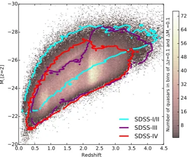
Finally, we present a density map of the DR14Q quasars in
the L − z plane in Fig.7. The area covered in this plane by each
phase of SDSS is also displayed. SDSS-I/II (cyan contour) has observed the brightest quasars at all redshifts. SDSS-III (purple contour) has observed up to two magnitudes deeper than SDSS-I/II, mostly at z > 2. SDSS-IV (red contour) is observing at the same depth as for SDSS-III but at lower redshift, i.e. focusing on the redshift range 0.8–2.2.
7. Multi-wavelength cross-correlation
We provide multi-wavelength matching of DR14Q quasars to
several surveys: the FIRST radio survey (Becker et al. 1995),
the Galaxy Evolution Explorer (GALEX, Martin et al. 2005)
Fig. 5. Left panel: redshift distribution of DR14Q quasars (black thick histogram) in the range 0 ≤ z ≤ 5. The redshift distribution of quasars observed as part of SDSS-I/II is shown with a cyan histogram. The redshift distributions of quasars observed as part of SDSS-III (purple his-togram) and SDSS-IV (red hishis-togram) are also displayed. Right panel: redshift distributions of all CORE quasars that are part of DR14Q (dark blue histogram), CORE quasars observed as part of SDSS-IV/eBOSS (light blue histogram), all PTF quasars (brown histogram), PTF quasars observed as part of SDSS-IV/eBOSS (orange histogram), SDSS-IV/TDSS quasars (green histogram) and quasars observed as part of ancillary programs (pink histogram). Some quasars can be selected by several target selection algorithms, hence the cumulative number of quasars in a single redshift bin can exceed the total number in that bin. The bin size for both panels is∆z = 0.05.
Fig. 6. Left panel: distribution of r-band magnitude corrected for Galactic extinction using theSchlafly & Finkbeiner(2011) dust maps for all DR14Q quasars (thick black histogram), quasars observed during SDSS-I/II (cyan histogram), SDSS-III (purple histogram) and SDSS-IV (red histogram). Right panel: distribution of r-band magnitude corrected for Galactic extinction for all CORE quasars (dark blue histogram), CORE quasars observed as part of SDSS-IV only (light blue histogram), all PTF quasars (brown histogram), PTF quasars observed as part of SDSS-IV only (orange histogram), SDSS-IV/TDSS quasars (green histogram), and quasars selected as part of ancillary programs (pink histogram). A given quasar can be selected by several target selection algorithms, hence the cumulative number of quasars in a r-band magnitude bin can exceed the total number of objects in it. The bin size for both panels is∆r = 0.1.
(Cutri et al. 2003; Skrutskie et al. 2006), the UKIRT Infrared
Deep Sky Survey (UKIDSS;Lawrence et al. 2007), the WISE
(Wright et al. 2010), the ROSAT All-Sky Survey (RASS;Voges et al. 1999, 2000), and the seventh data release of the Third
XMM-NewtonSerendipitous Source Catalog (Rosen et al. 2016).
7.1. FIRST
As for the previous SDSS-III/BOSS quasar catalogs, we matched the DR14Q quasars to the latest FIRST catalog (December 2014;
Becker et al. 1995) using a 200 matching radius. We report the flux peak density at 20 cm and the S/N of the detection. Among the DR14Q quasars, 73 126 lie outside of the FIRST footprint and have their FIRST_MATCHED flag set to −1.
A total of 18 273 quasars have FIRST counterparts in DR14Q. We estimate the fraction of chance superpositions
by offsetting the declination of DR14Q quasars by 20000. We
then re-match to the FIRST source catalog. We conclude that there are about 0.2% of false positives in the DR14Q-FIRST matching.
Fig. 7. Density map of the DR14Q quasars in the L − z plane. The color map indicates the number of DR14Q quasars in bins of∆z = 0.1 and ∆Mi[z= 2] = 0.1. Colored contours correspond to the envelope in the
L − zplane for each iteration of SDSS. The absolute magnitudes assume H0= 70 km s−1Mpc−1and the K-correction is given byRichards et al.
(2006), who define K (z= 2) = 0.
7.2. GALEX
As for DR12Q, GALEX (Martin et al. 2005) images are
force-photometered (from GALEX DR 5) at the SDSS-DR8 centroids (Aihara et al. 2011), such that low S/N PSF fluxes of objects not detected by GALEX are recovered, for both the FUV (1350– 1750 Å) and NUV (1750–2750 Å) bands when available. A total of 382 838 quasars are detected in the NUV band, 304 705 in the FUV band and 515 728 have non-zero fluxes in both bands. 7.3. 2MASS
We cross-correlate DR14Q with the All-Sky data release Point
Source catalog (Skrutskie et al. 2006) using a matching radius
of 200. We report the Vega-based magnitudes in the J, H and
K-bands and their error together with the S/N of the detections. We also provide the value of the 2MASS flag rd_flg[1], which defines the peculiar values of the magnitude and its error for each band3.
There are 16 427 matches in the catalog. This number is quite small compared with the number of DR14Q quasars because the sensitivity of 2MASS is much less than that of SDSS. Applying
the same method as described in Sect.7.1, we estimate that 0.8%
of the matches are false positives. 7.4. WISE
We matched the DR14Q to the AllWISE Source Catalog4
(Wright et al. 2010;Mainzer et al. 2011). Our procedure is the
same as in DR12Q, with a matching radius of 2.000. There are
401 980 matches from the AllWISE Source Catalog. Following the procedure described in Sect.7.1, we estimate the rate of false positive matches to be about 2%, which is consistent with the findings ofKrawczyk et al.(2013).
3 seehttp://www.ipac.caltech.edu/2mass/releases/allsky/ doc/explsup.htmlfor more details.
4 http://wise2.ipac.caltech.edu/docs/release/allwise/
We report the magnitudes, their associated errors, the S/N of the detection and reduced χ2of the profile-fitting in the four WISE bands centered at wavelengths of 3.4, 4.6, 12 and 22 µm. These magnitudes are in the Vega system, and are measured with profile-fitting photometry. We also report the WISE catalog con-tamination and confusion flag, cc_flags, and their photometric quality flag, ph_qual. As suggested on the WISE “Cautionary
Notes” page5, we recommend using only those matches with
cc_flags = “0000” to exclude objects that are flagged as spu-rious detections of image artifacts in any band. Full details about quantities provided in the AllWISE Source Catalog can be found on their online documentation6.
7.5. UKIDSS
As for DR12Q, near infrared images from the UKIRT Infrared
Deep Sky Survey (UKIDSS; Lawrence et al. 2007) are
force-photometered.
We provide the fluxes and their associated errors, expressed
in W m−2Hz−1, in the Y, J, H and K bands. The conversion to
the Vega magnitudes, as used in 2MASS, is given by the formula:
magX = −2.5 × log fX
f0,X× 10−26, (2)
where X denotes the filter and the zero-point values f0,X are
2026, 1530, 1019 and 631 for the Y, J, H and K bands respec-tively.
A total of 112 012 quasars are detected in at least one of the four bands Y, J, H or K. 111 083 objects are detected in the Y band, 110 691 in the J band, 110 630 in H band, 111 245 in the K band and 108 392 objects have non-zero fluxes in the four bands. Objects with zero fluxes lie outside the UKIDSS footprint. The UKIDSS limiting magnitude is K ∼ 18 (for the Large Area Sur-vey) while the 2MASS limiting magnitude in the same band is ∼15.3. This difference in depth between the two surveys explains the large difference in the numbers of matches with DR14Q. 7.6. ROSAT
As was done for the previous SDSS-III/BOSS quasar catalogs, we matched the DR14Q quasars to the ROSAT all sky survey Faint (Voges et al. 2000) and Bright (Voges et al. 1999) source
catalogs with a matching radius of 3000. Only the most reliable
detections are included in our catalog: when the quality detec-tion is flagged as potentially problematic, we do not include the match. A total of 8655 quasars are detected in one of the RASS catalogs. As for the cross-correlations described above, we esti-mate that 2.1% of the RASS-DR14Q matches are due to chance superposition.
7.7. XMM-Newton
DR14Q was cross-correlated with the seventh data release of the
Third XMM-Newton Serendipitous Source Catalog (Rosen et al.
2016)7 (3XMM-DR7) using a standard 5.000 matching radius.
For each of the 14 736 DR14Q quasars with XMM-Newton counterparts, we report the soft (0.2–2 keV), hard (4.5–12 keV)
5 http://wise2.ipac.caltech.edu/docs/release/allsky/ expsup/sec1_4b.html#unreliab 6 http://wise2.ipac.caltech.edu/docs/release/allsky/ expsup/sec2_2a.html 7 http://xmmssc.irap.omp.eu/Catalogue/3XMM-DR7/3XMM_ DR7.html
and total (0.2–12 keV) fluxes, and associated errors, that were computed as the weighted average of all the detections in the three XMM-Newton cameras (MOS1, MOS2, PN). Correspond-ing observed X-ray luminosities are computed in each band and are not absorption corrected. All fluxes and errors are expressed
in erg cm−2s−1and luminosities are computed using the redshift
value Z from the present catalog.
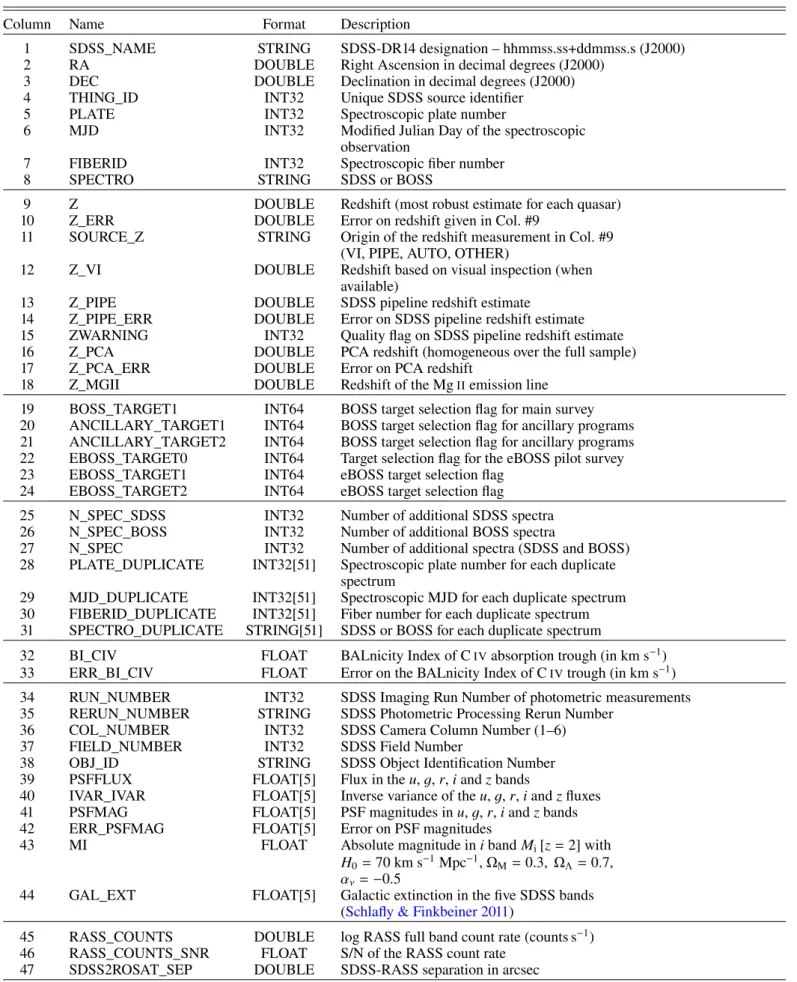
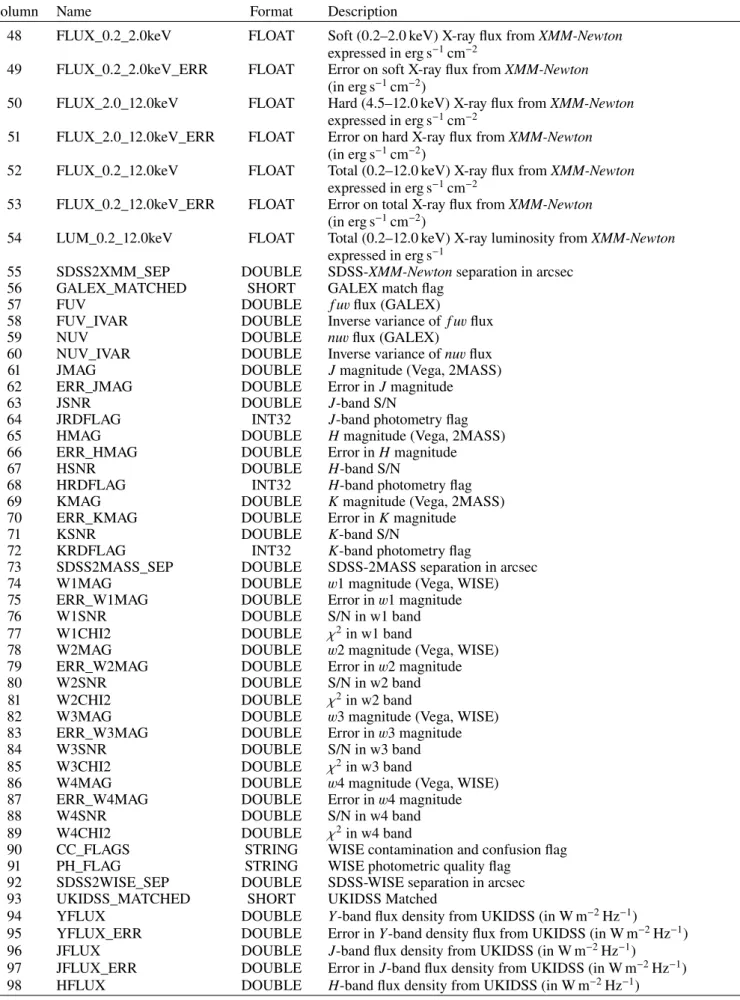
8. Description of the DR14Q catalog
The DR14Q catalog is publicly available on the SDSS public
website8as a binary FITS table file. All the required
documenta-tion (format, name, unit for each column) is provided in the FITS
header. It is also summarized in TableA.1.
Notes on the catalog columns:
1. The DR14 object designation, given by the format SDSS Jhhmmss.ss+ddmmss.s; only the final 18 characters are listed in the catalog (i.e. the character string “SDSS J” is dropped). The coordinates in the object name follow IAU convention and are truncated, not rounded.
2–3. The J2000 coordinates (Right Ascension and Decli-nation) in decimal degrees. The astrometry is from SDSS-DR14 (Abolfathi et al. 2017).
4. The 64-bit integer that uniquely describes the objects that are listed in the SDSS (photometric and spectroscopic) catalogs (THING_ID).
5–7. Information about the spectroscopic observation (Spec-troscopic plate number, Modified Julian Date, and spectro-scopic fiber number) used to determine the characteristics of the spectrum. These three numbers are unique for each spec-trum, and can be used to retrieve the digital spectra from the public SDSS database. When an object has been observed more than once, we selected the best quality spectrum as defined by the SDSS pipeline (Bolton et al. 2012), i.e. with SPECPRIMARY = 1.
8. DR14Q compiles all spectroscopic observations of quasars, including SDSS-I/II spectra taken with a different spectrograph. For spectra taken with the SDSS
spectro-graphs, i.e. spectra released prior to SDSS-DR8 (Aihara
et al. 2011), SPECTRO is set to “SDSS”. For spectra taken
with the BOSS spectrographs (Smee et al. 2013), SPECTRO
is set to “BOSS”.
9–11. Quasar redshift (Col. #9) and associated error (Col. #10). This redshift estimate is the most robust for quasar cataloging purposes and it is used as a prior for refined redshift measurements. Values reported in Col. #9 are from different sources: the outcome of the automated
procedure described in Sect. 3.2, visual inspection or the
BOSS pipeline (Bolton et al. 2012). The origin of the redshift value is given in Col. #11 (AUTO, VI and PIPE respectively). 12. Redshift from the visual inspection, Z_VI, when avail-able. All SDSS-I/II/III quasars have been visually inspected. About 7% of SDSS-IV quasars have been through this process (see Sect.3.2for more details).
13–15. Redshift (Z_PIPE, Col. #13), associated error (Z_PIPE_ERR, Col. #14) and quality flag (ZWARNING,
8 http://www.sdss.org/dr14/algorithms/qso_catalog
Col. #15) from the BOSS pipeline (Bolton et al. 2012).
ZWARNING > 0 indicates uncertain results in the redshift-fitting code.
16–17. Automatic redshift estimate (Z_PCA, Col. #16) and associated error (Z_PCA_ERR, Col. #17) using a linear
com-bination of four principal components (see Sect. 4 for
details). When the velocity difference between the automatic PCA and visual inspection redshift estimates is larger than 5000 km s−1, this PCA redshift and error are set to −1.
18. Redshifts measured from the MgIIemission line from a
linear combination of five principal components (see Pâris
et al. 2012). The line redshift is estimated using the posi-tion of the maximum of each emission line, contrary to Z_PCA (Col. #16) which is a global estimate using all the information available in a given spectrum.
19–24. The main target selection information for SDSS-III/BOSS quasars is tracked with the BOSS_TARGET1 flag
bits (Col. #19; see Table 2 in Ross et al. 2012, for a
full description). SDSS-III ancillary program target selec-tion is tracked with the ANCILLARY_TARGET1 (Col. #20) and ANCILLARY_TARGET2 (Col. #21) flag bits. The bit values and the corresponding program names are listed in Dawson et al. (2013), and Alam et al. (2015). Tar-get selection information for the SDSS-IV pilot survey
(SEQUELS; Dawson et al. 2016; Myers et al. 2015) is
tracked with the EBOSS_TARGET0 flag bits (Col. #22). Finally, target selection information for SDSS-IV/eBOSS, SDSS-IV/TDSS and SDSS-IV/SPIDERS quasars is tracked with the EBOSS_TARGET1 and EBOSS_TARGET2 flag bits. All the target selection bits, program names and associated
references are summarized in Table1.
25–31. If a quasar in DR14Q was observed more than once by SDSS-I/II/III/IV, the number of additional SDSS-I/II spectra is given by N_SPEC_SDSS (Col. #25), the number of additional SDSS-III/IV spectra by N_SPEC_BOSS (Col. #26), and the total number by N_SPEC (Col. #27). The asso-ciated plate (PLATE_DUPLICATE, MJD (MJD_DUPLICATE), fiber (FIBERID_DUPLICATE) numbers, and spectrograph information (SPECTRO_DUPLICATE) are given in Cols. #28, 29, 30 and 31 respectively. If a quasar was observed N times in total, the best spectrum is identified in Cols. #5– 7, the corresponding N_SPEC is N − 1, and the first
N −1 columns of PLATE_DUPLICATE, MJD_DUPLICATE,
FIBERID_DUPLICATE, and SPECTRO_DUPLICATE are filled with relevant information. Remaining columns are set to −1.
32–33. BALnicity Index (BI;Weymann et al. 1991; Col. #32)
for CIVtroughs, and associated error (Col. #33), expressed
in km s−1. See definition in Sect.5. The BALnicity Index is measured for quasars with z > 1.57 only, so that the trough enters into the BOSS wavelength region. In cases with poor fits to the continuum, the BALnicity Index and its error are set to −1.
34. The SDSS Imaging Run number (RUN_NUMBER) of the photometric observation used in the catalog.
35–38. Additional SDSS processing information: the photo-metric processing rerun number (RERUN_NUMBER, Col. #35); the camera column (1–6) containing the image of the object (COL_NUMBER, Col. #36), the field number of the run con-taining the object (FIELD_NUMBER, Col. #37), and the object
identification number (OBJ_ID, Col. #38; see Stoughton et al. 2002, for descriptions of these parameters).
39–40. DR14 PSF fluxes, expressed in nanomaggies9, and
inverse variances (not corrected for Galactic extinction) in the five SDSS filters.
41–42. DR14 PSF AB magnitudes (Oke & Gunn 1983) and
errors (not corrected for Galactic extinction) in the five SDSS filters. These magnitudes are Asinh magnitudes as defined inLupton et al.(1999).
43. The absolute magnitude in the i band at z= 2 calculated
using a power-law (frequency) continuum index of −0.5. The
K-correction is computed using Table 4 fromRichards et al.
(2006). We use the SDSS primary photometry to compute
this value.
44. Galactic extinction in the five SDSS bands based on Schlafly & Finkbeiner(2011).
45. The logarithm of the vignetting-corrected count rate
(photons s−1) in the broad energy band (0.1–2.4 keV) from
the ROSAT All-Sky Survey Faint Source Catalog (Voges
et al. 2000) and the ROSAT All-Sky Survey Bright Source
Catalog (Voges et al. 1999). The matching radius was set to
3000(see Sect.7.6).
46. The S/N of the ROSAT measurement.
47. Angular separation between the SDSS and ROSAT All-Sky Survey locations (in arcsec).
48–49. Soft X-ray flux (0.2–2 keV) from XMM-Newton matching, expressed in erg cm−2s−1, and its error. In the case of multiple observations, the values reported here are the weighted average of all the XMM-Newton detections in this band.
50–51. Hard X-ray flux (4.5–12 keV) from XMM-Newton
matching, expressed in erg cm−2s−1, and its error. In the
case of multiple observations, the reported values are the weighted average of all the XMM-Newton detections in this band.
52–53. Total X-ray flux (0.2–12 keV) from the three
XMM-Newton CCDs (MOS1, MOS2 and PN), expressed in
erg cm−2s−1, and its error. In the case of multiple
XMM-Newtonobservations, only the longest exposure was used to
compute the reported flux.
54. Total X-ray luminosity (0.2–12 keV) derived from the
flux computed in Col. #52, expressed in erg s−1. This value
is computed using the redshift value reported in Col. #9 and is not absorption corrected.
55. Angular separation between the XMM-Newton and SDSS-DR14 locations, expressed in arcsec.
56. If a SDSS-DR14 quasar matches with GALEX pho-tometering, GALEX_MATCHED is set to 1, 0 if no GALEX match.
9 See http://www.sdss.org/dr14/algorithms/magnitudes/ #nmgy
57–60. UV fluxes and inverse variances from GALEX, aperture-photometered from the original GALEX images in the two bands FUV and NUV. The fluxes are expressed in nanomaggies.
61–62. The J magnitude and error from the Two Micron All
Sky Survey All-Sky data release Point Source Catalog (Cutri
et al. 2003) using a matching radius of 2.000(see Sect.7.3). A non-detection by 2MASS is indicated by a “0.000” in these columns. The 2MASS measurements are in Vega, not AB, magnitudes.
63–64. S/N in the J band and corresponding 2MASS jr_d flag that gives the meaning of the peculiar values of the magnitude and its error10.
65–68. Same as 61–64 for the H-band. 69–72. Same as 61–64 for the K-band.
73. Angular separation between the SDSS-DR14 and 2MASS positions (in arcsec).
74–75. The w1 magnitude and error from the Wide-field
Infrared Survey Explorer (WISE; Wright et al. 2010)
All-WISE data release Point Source Catalog using a matching radius of 200.
76–77. S/N and χ2in the WISE w1 band.
78–81. Same as 74–77 for the w2-band. 82–85. Same as 74–77 for the w3-band. 86–89. Same as 74–77 for the w4-band. 90. WISE contamination and confusion flag. 91. WISE photometric quality flag.
92. Angular separation between SDSS-DR14 and WISE positions (in arcsec).
93. If a SDSS-DR14 quasar matches UKIDSS aperture-photometering data, UKIDSS_MATCHED is set to 1, it is set to 0 if UKIDSS match.
94–101. Flux density and error from UKIDSS, aperture-photometered from the original UKIDSS images in the four bands Y (Cols. #94–95), J (Cols. #96–97), H (Cols. #98–99) and K (Cols. #100–101). The fluxes and errors are expressed in W m−2Hz−1.
102. If there is a source in the FIRST radio catalog
(ver-sion December 2014) within 2.000of the quasar position, the
FIRST_MATCHED flag provided in this column is set to 1, 0 if not. If the quasar lies outside of the FIRST footprint, it is set to −1.
103. The FIRST peak flux density, expressed in mJy. 104. The S/N of the FIRST source whose flux is given in Col. #103.
105. Angular separation between the SDSS-DR14 and FIRST positions (in arcsec).
10 seehttp://www.ipac.caltech.edu/2mass/releases/allsky/ doc/explsup.html