HAL Id: hal-03210218
https://hal.archives-ouvertes.fr/hal-03210218
Submitted on 28 Apr 2021
HAL is a multi-disciplinary open access
archive for the deposit and dissemination of
sci-entific research documents, whether they are
pub-lished or not. The documents may come from
teaching and research institutions in France or
abroad, or from public or private research centers.
L’archive ouverte pluridisciplinaire HAL, est
destinée au dépôt et à la diffusion de documents
scientifiques de niveau recherche, publiés ou non,
émanant des établissements d’enseignement et de
recherche français ou étrangers, des laboratoires
publics ou privés.
measurements in the UTLS – Part 1: Method
description and application at Payerne, Switzerland
J. Staufer, J. Staehelin, R. Stübi, T. Peter, F. Tummon, V. Thouret
To cite this version:
J. Staufer, J. Staehelin, R. Stübi, T. Peter, F. Tummon, et al.. Trajectory matching of ozonesondes
and MOZAIC measurements in the UTLS – Part 1: Method description and application at
Pay-erne, Switzerland. Atmospheric Measurement Techniques, European Geosciences Union, 2013, 6 (12),
pp.3393-3406. �10.5194/amt-6-3393-2013�. �hal-03210218�
www.atmos-meas-tech.net/6/3393/2013/ doi:10.5194/amt-6-3393-2013
© Author(s) 2013. CC Attribution 3.0 License.
Atmospheric
Measurement
Techniques
Trajectory matching of ozonesondes and MOZAIC measurements in
the UTLS – Part 1: Method description and application at Payerne,
Switzerland
J. Staufer1,*, J. Staehelin1, R. Stübi2, T. Peter1, F. Tummon1, and V. Thouret3
1Institute for Atmospheric and Climate Science, ETH Zurich, Zurich, Switzerland 2Federal Office of Meteorology and Climatology MeteoSwiss, Aerological Station,
Payerne, Switzerland
3Laboratoire d’Aérologie, Université de Toulouse, CNRS, Toulouse, France
*now at: Laboratoire des Sciences du Climat et de l’Environnement, CEA-CNRS-UVSQ, IPSL, Gif-sur-Yvette, France
Correspondence to: J. Staufer (johannes.staufer@lsce.ipsl.fr)
Received: 2 June 2013 – Published in Atmos. Meas. Tech. Discuss.: 1 August 2013 Revised: 24 October 2013 – Accepted: 8 November 2013 – Published: 9 December 2013
Abstract. With the aim of improving ozonesonde
observa-tions in the upper troposphere/lower stratosphere (UTLS), we use three-dimensional forward and backward trajectories, driven by ERA-Interim wind fields to match and compare ozonesonde measurements at Payerne (Switzerland) with ob-servations from the MOZAIC aircraft program from 1994– 2009. The uncertainties associated with the sonde–MOZAIC match technique were assessed using “self-matches”, i.e. matches of instruments of the same type, such as MOZAIC– MOZAIC. Despite strong vertical gradients of ozone at the tropopause, which render the match approach difficult, the method provides excellent results, showing mean differ-ences between different MOZAIC aircraft of ±2 % (typi-cally with a few hours between the up- and downstream match points). Matches between MOZAIC aircraft and Pay-erne ozonesondes show an agreement of ±5 % for sondes equipped with electrochemical concentration cells (ECC) and between < 5 % (not scaled to total ozone) and < 10 % (scaled) for the Brewer–Mast (BM) sondes after 1998. Prior to 1998, BM sondes show an offset of around 20 % (scaled). No break can be identified through the change from the BM to ECC sonde types in September 2002. A comparison of BM sondes with ozone measurements from the NOXAR B747 project for the period 1995–1996 show a smaller offset of around 15 % (scaled), which may indicate a small drift in the MOZAIC calibration.
1 Introduction
Ozone (O3) in the upper troposphere/lower stratosphere
(UTLS) is an important element of the climate system. Per-turbations in the O3distributions in this region have strongest
impact on surface temperatures when they are introduced around the tropopause (Lacis et al., 1990; Forster and Shine, 1997). Furthermore, modeling studies project greenhouse-gas-induced cooling of the stratosphere and an accelera-tion of stratospheric circulaaccelera-tion (Brewer–Dobson circulaaccelera-tion) (e.g. Shepherd, 2008), which could, in addition to the recov-ery of the O3 layer due to declining halogen abundances,
significantly increase extra-tropical UTLS O3over the 21st
century (Hegglin and Shepherd, 2009). The documentation of possible long-term changes in UTLS O3 is therefore
vi-tal, but the complex dynamics and chemistry of the UTLS mean that observations need to have high vertical and hori-zontal spatial resolution, as well as high temporal resolution, to allow good comparison with numerical simulations.
Different in-situ techniques for measuring UTLS O3
con-centrations, such as balloon-borne ozonesondes, are avail-able. Although originally designed for measuring O3 for
large-scale stratospheric dynamical studies (e.g. Smit, 2002), they have become invaluable for measuring changes in the vertical distribution of O3. In particular, their high
verti-cal resolution provides observations of the pronounced ver-tical ozone gradients in the UTLS. A typical sonde ascent rate is about 4–6 m s−1 leading to an altitude resolution
of 100–200 m. The low O3 concentrations below the
tropopause, however, remain challenging. Special emphasis needs to be placed on data quality and consistency, since ev-ery sounding is made with a new instrument and a number of modifications, such as the use of different sensor types and radiosondes, or changing preflight or post flight data pro-cessing procedures, may have affected ozonesonde records (Smit et al., 2007).
Representative, high quality in-situ O3measurements can
also be obtained from regular aircraft measurements, for ex-ample, from the MOZAIC programme (Measurements of ozone, water vapour, carbon monoxide and nitrogen oxides by in-service Airbus aircraft, Marenco et al., 1998; Thouret et al., 1998a, b, 2006). The MOZAIC programme, in opera-tion since August 1994, equipped commercial airliners with an accurate UV photometer to measure ozone concentrations. Cruise altitude of the aircraft range between 9–13 km, co-inciding with tropopause heights at mid-latitudes. Recently, MOZAIC has become a part of the IAGOS (In-service Air-craft for a Global Observing System, http://www.iagos.org) programme. IAGOS observations additionally include cloud droplets (number and size) and optionally either CO2 and
CH4, aerosols, NOxor NOy. Long-term, global scale
obser-vations will be provided by a fleet of 10–20 long-range in-service aircraft operated by several international airlines.
Regular aircraft measurements of ozone and nitrogen ox-ides were also provided by the NOXAR (Nitrogen Ox-ides and Ozone along Air Routes project) programme us-ing a Swissair B747 as a measurus-ing platform (Brunner et al., 2001) in 1995–1997.
To assess the performance and quantify systematic differ-ences between different types of ozonesondes and ozoneson-des from different manufacturers, the environmental sim-ulation facility at the Juelich Research center was estab-lished as the World Meteorological Organization’s (WMO) World Calibration Center for ozonesondes (Smit et al., 2007). The facility allows simulation of flight conditions of ozone soundings up to 35 km by controlling pressure, temperature and O3 concentrations. Up to four
sound-ings can be simultaneously compared with an accurate UV-photometer. Detailed specifications of the environment chamber capabilities and measurements have been described by Smit et al. (2000, 2007).
Experiments performed during the Juelich Ozone Sonde Intercomparison Experiment (JOSIE 1996–2000, Smit and Kley, 1998; Smit and Straeter, 2004a, b; Smit et al., 2007) show that ECC (Electrochemical concentration cell) son-des have a positive bias of 5–10 % compared to the UV photometer, at conditions corresponding to 5–15 km. Some dependence on preflight preparation, manufacturer, elec-trochemical sensing solution strength, and data process-ing was also observed (Smit et al., 2007). Conversely, the BM (Brewer–Mast) sondes show a negative bias of −3 % at altitudes between 5–15 km, but a much higher scatter (Smit and Kley, 1998).
Generally, uncertainties of simulation chamber results are determined by randomly selecting sondes either from stocks or directly from the manufactures or the sounding sites. How-ever, results may not necessarily reflect their performance un-der operational field conditions (Smit and Kley, 1998). A dif-ferent approach was used by Bodeker et al. (1998), who ap-plied a Monte Carlo error analysis to estimate the overall un-certainties of ECC sondes. They derived an uncertainty of 5–10 % at mid-latitude tropopause altitudes, depending on sonde manufacturers. Earlier intercomparison of ozoneson-des with an UV photometer (e.g. Hilsenrath et al., 1986) es-timated measurement accuracies of 10 % in the troposphere and 5 % in the stratosphere up to 10 hPa.
The quality of the ozonesonde time series’ is, however, problematic. This is especially the case when data from the UTLS are used for long-term trend analysis, given the high variability in this region. Furthermore, the use of data may also strongly depend on data selection criteria, for exam-ple, criteria with respect to the correction factor (CF) (Logan et al., 1999). By comparing UTLS ozone climatologies with measurements from the 1970s commercial aircraft Global Atmospheric Sampling Programme (GASP) and MOZAIC observations from the 1990s, Schnadt Poberaj et al. (2009) showed that the irregular behaviour of the European BM son-des led to differences in the long-term changes of ozone over Europe. Recently, Logan et al. (2012) compared monthly-mean time series’ from European sounding sites with time series’ from both neighbouring Alpine surface measurements and MOZAIC observations at nearby airports. They report large biases between MOZAIC and the BM sondes from 1994–1996 in the free troposphere, and conclude that “BM sonde data are not useful for deriving reliable tropospheric trends prior to about 1998”.
The aim of this paper is to examine the feasibility of us-ing trajectory analysis to allow systematic comparisons of O3soundings with commercial aircraft measurements at
al-titudes between 4–14 km, and to compare both instrument types over the entire period for which MOZAIC observa-tions are available. Since both these types of ozone mea-surements are commonly used to investigate short- and long-term ozone changes (e.g. Tarasick et al., 2005; Thouret et al., 2006; Schnadt Poberaj et al., 2009; Logan et al., 2012), as well as to validate chemistry climate models, and remote-sensing instruments (e.g. Law et al., 2000; Brunner et al., 2003; Liu et al., 2006), it is crucial to understand the degree of consistency between both datasets.
We make use of the “MATCH technique”, an approach that matches two sets of observations by searching for air parcels sampled by both observations over the course of a few days using particular match criteria. Conceptually, this approach is derived from the MATCH technique ap-plied to estimate ozone loss rates in the Arctic polar vor-tex (Rex et al., 1998; Morris et al., 2005, and references therein). A similar concept is “trajectory hunting”, as used by Danilin et al. (2000, 2002a, b), which refers to the fact
that trajectories originating from one platform are “hunted” for matches by other observation platforms.
This approach can be applied to any ozonesonde series provided that enough commercial aircraft measurements are available for comparison. For this work we use ozonesonde data from Payerne, Switzerland, to serve as an introduction and test of this method. Typically, 2–3 ozonesondes per week are launched at Payerne and in September 2002 BM sondes were replaced by ECC sondes. In this paper, we assess the reliability and consistency of the Payerne ozonesonde time series, checking and evaluating the data with MOZAIC mea-surements for the eight years available before and after the BM-ECC transition. In Staufer et al. (2013), the same method is applied to other ozonesonde sites.
2 Methodology and measurements
2.1 Ozone measurements from regular aircraft
2.1.1 MOZAIC
The MOZAIC programme, which begun in 1994, was es-tablished to obtain a large experimental data base of ozone and water vapour observations utilising automatic instru-ments installed on five commercial long-range Airbus airlin-ers (Marenco et al., 1998). The ozone instrument is described in detail by Thouret et al. (1998a). Here we briefly summarise the main aspects. The MOZAIC ozone analysers are dual-beam UV absorption instruments from Thermo Environment. They have a response time of 4 s, a detection limit of 2 ppbv, and an accuracy of ±2 %. The uncertainty has been estimated at ±[2 % + 2 ppbv]. For O3=100 ppbv, this means an
un-certainty of ±4 ppbv. Quality assurance and control proce-dures have not changed since 1994 and involve a periodi-cal (about 12 months) laboratory periodi-calibration with a reference analyser at the National Institute of Standards and Technol-ogy, in France, as well as an in-flight check with a built-in ozone generator to detect any drift in instrument efficiency.
The MOZAIC data used here were downloaded in March 2010. At this time data were available until March 2009 and comprised 31 534 flights from August 1994 to March 2009. We used data integrated over 1 min. At cruise altitude, which approximately coincides with tropopause al-titude in the mid-laal-titudes (9–13 km), this corresponds to a horizontal resolution of about 15 km.
2.1.2 NOXAR
Within the framework of the Swiss NOXAR (Nitrogen Ox-ides and Ozone along Air Routes) project (Brunner et al., 2001) a commercial airliner (B-747-357 Combi operated by Swissair) was equipped with a fully automated system (ECO PHYSICS CLD 780 TR) for measuring NO, NO2, and O3in
the Northern Hemisphere UTLS. Measurements were made from May 1995 to May 1996 and from August to
Novem-ber 1997, when the NOXAR airliner participated in the Eu-ropean POLINAT-2 (Pollution from Aircraft Emissions in the North Atlantic Flight Corridor) project.
Similar to MOZAIC, the ozone analyser uses the UV-absorption of O3 at 253.7 nm. The response time of the
analyser is 4 s with a total accuracy of ±6 % (Dias-Lalcaca et al., 1998). NOXAR data were obtained from the
ETH-meg database (http://www.ETH-megdb.ethz.ch), from which 2 min
averages are available (Brunner et al., 2003). One quasi-simultaneous flight of MOZAIC and NOXAR aircraft over the North Atlantic on 20 December 1995 revealed excellent agreement for the observed range of O3 concentrations
be-tween 40 and 400 ppbv (Dias-Lalcaca et al., 1998).
2.2 Ozone measurements from balloon-borne ozonesondes
2.2.1 Measurement principles
Several types of ozonesondes have been developed, two of which have coexisted over the last 40 yr and which are still in use: the BM sonde (Brewer and Milford, 1960) and the ECC sonde (Komhyr, 1969). Although the measurement principle of both electrochemical sonde types is similar – namely the titration of O3in a potassium iodide (KI) sensing solution –
at present, the ECC sonde type dominates the global monitor-ing network, since they are less sensitive to preflight prepara-tions and manufacturing aspects than BM sondes (Smit and Kley, 1998). Overall errors and uncertainties in the sound-ings are thought to originate from the background current of electrochemical cells, degrading of the pump efficiency with lower ambient pressures and inaccurate pump tempera-ture measurements. Whereas the degrading of the pump effi-ciency predominantly affects the upper part of the profile, the background current produces the largest deviation below the tropopause and in the tropical troposphere when O3
concen-tration is low. The background signal depends strongly on the sonde preparation, especially for ECC sondes (e.g. Vömel and Diaz, 2010).
2.2.2 Data processing methods at Payerne
The BM sondes at Payerne were prepared and processed following WMO (World Meteorological Organization) stan-dardized operating procedures (SOP), as described by Claude et al. (1987). However, the pump temperature was set to 280 K instead of 300 K because the packages specially de-signed for the Swiss meteorological sondes did not protect the BM pump in the same way as the original BM-VIZ pack-ages (Jeannet et al., 2007; Stübi et al., 2008). The SOP in-clude scaling the whole profile to a near-by independent to-tal ozone measurement which reduces the sonde variabil-ity and corrects for the low bias of the BM’s ozone col-umn. The procedure also requires an estimation of the O3
O3measurements has been debated (e.g. SPARC/IOC/GAW,
1998; De Backer et al., 1998; Thouret et al., 1998a), since the scaling depends primarily on stratospheric O3and the
as-sumptions made to estimate the ozone column above burst al-titude. Any errors in the column measurement therefore can be carried over into the whole profile, in particular since (un-scaled) BM sondes tend to underestimate ozone in the strato-sphere more strongly than in the UTLS (see Stübi et al., 2008, their Fig. 8).
The total ozone normalization at Payerne is based on daily averages from Dobson spectrophotometer measurements at Arosa (200 km east of Payerne, 1860 m a.s.l.), or, if Dob-son data are not available, on satellite measurements (Jean-net et al., 2007). For the calculation of the correction factor the height difference between Payerne and Arosa is taken into account using only ozonesonde measurements above the Arosa height. Strong horizontal ozone gradients between Payerne and Arosa can occasionally occur, but are expected to cancel out in the mean values (see also Jeannet et al., 2007).
Arosa total ozone columns, together with many other ground-based Dobson stations, have recently been used by Labow et al. (2013) for comparison with reprocessed SBUV, BUV and SBUV-2 data. Typically, their time series’ agree within 1 % over the past 40 yr (see, for example, their Figs. 6 and 7). Over the last decade, the bias even approaches zero.
Since September 2002, ECC ozonesondes (model type ENSCI-2Z, 0.5 % KI half-buffered sensing solution) have been operated at Payerne. The preparation and processing of the ECC sondes is described in detail by Stübi et al. (2008). Essentially, the background current is measured at ground level prior to launch and is assumed to be constant during the ascents. The thermistor for measuring pump temperature during flight is placed inside the Teflon block close to the piston. The pump efficiency correction was selected accord-ing to the manufacturer’s recommendations (Komhyr et al., 1995). ECC sondes are usually not scaled to column ozone.
2.3 Comparison method
This study is based on the concept of identifying air masses which have been sampled for O3 measurements by both
ozonesondes and MOZAIC aircraft. For our comparison, the signal of the ozonesonde, ozone partial pressure, is converted to molecule number density using pressure information from the radiosonde. Longitude and latitude position along the bal-loon flight track are usually not reported to archives, hence, we reconstruct the balloon’s pathway if wind speed and di-rection were reported. If unavailable, a purely vertical as-cent was assumed. For each launch we calculate the thermal tropopause defined as the lowest height of an at least 2 km thick layer, in which the temperature lapse rate 0 = −∂T /∂z is less than 2 K km−1 (World Meteorological Organization, 1957). Subsequently, we define the UTLS as the region cen-tred ±125 hPa around the local tropopause. Beginning from
the bottom of the UTLS up to its top, fully three-dimensional trajectories (both forward and backward) are initialised at 5 hPa intervals from the bottom to the top of the UTLS using the trajectory tool LAGRANTO (Wernli and Davies, 1997) to trace the air masses in each direction for 144 h (6 days).
LAGRANTO has performed well in several other studies focusing on the UTLS (e.g. Wernli and Bourqui, 2002; Cui et al., 2009). For our study, it is driven by 6 hourly wind fields from ECMWF’s ERA-Interim reanalysis with a horizontal resolution of 1◦longitude ×1◦latitude and 61 hybrid verti-cal levels. Although there are several numeriverti-cal models with better spatio-temporal resolution, we use ERA-Interim to en-sure that the results are independent of changes in the under-lying model. The temporal index for the tracing output is set to one minute to be consistent with MOZAIC observations.
Trajectories are then searched for matches with MOZAIC using match criteria that specify the maximum horizontal and vertical distance between trajectory and aircraft. Poten-tial temperature 2 is used for the vertical distance. See below for the match criteria used.
Matches are of different quality since trajectory errors typically accumulate with time (i.e. the further the aircraft observation is in time from the ozonesonde observation). A weighting is therefore introduced to account for the re-duced accuracy of the trajectories. Along each trajectory we collect all MOZAIC observations satisfying the match cri-teria, calculate the weighted mean and compare it to the point measurement of the sonde at initialization of the tra-jectory. We use the time lag between the MOZAIC observa-tions and the sounding for the weights, giving more weight to MOZAIC observations that are closer to the soundings. Thus, for each trajectory the weighted mean y is calculated according to y = PM i=1wiyi PM i=1wi , (1)
where M is the number of matches along one trajectory. wi is the weight of the individual aircraft observation yi and is obtained by
wi=
|t∗−1t |
t∗ , (2)
where t∗is the duration of the trajectories, 144 h, and 1t the time lag between aircraft observation and the sonde.
We assume that O3behaves as a passive tracer for the
du-ration of the trajectories. This is a critical assumption, but justified because the lifetime of Ox in the free troposphere
varies from days to months, depending on season and ambi-ent NOxconcentrations (Liu et al., 1987). In the lower
strato-sphere the photochemical lifetime is even longer, i.e. sev-eral months. Any trajectories that descend or ascend more than 450 hPa within six or less days are excluded. This ex-cludes deep stratospheric intrusions and avoids sampling pol-luted air masses transported in warm conveyor belts. Such
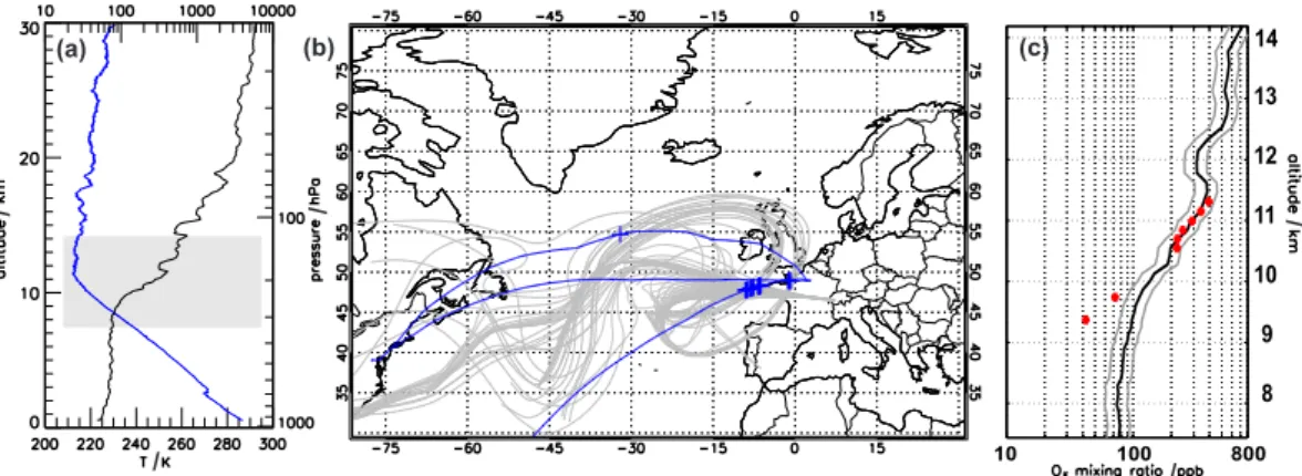
Fig. 1. (a) Ozone (black) and temperature (blue) profiles measured at Payerne on 18 April 1995. The gray
area indicates the UTLS (±125 hPa above and below the tropopause). (b) Plot of the 6 day backward trajectories. The blue solid lines denote the flight paths of three MOZAIC aircraft for which matches were found. Matches are denoted by blue plus signs. (c) UTLSO3as a function of altitude, as observed
by the sonde. Gray solid lines denote the 20 % uncertainty range of the soundings. Each red dot denotes the weighted mean (y) of the aircraft observations along respective trajectories.
26
Fig. 1. (a) Ozone (black) and temperature (blue) profiles measured at Payerne on 18 April 1995. The gray area indicates the UTLS (±125 hPa
above and below the tropopause). (b) Plot of the 6 day backward trajectories. The blue solid lines denote the flight paths of three MOZAIC aircraft for which matches were found. Matches are denoted by blue plus signs. (c) UTLS O3as a function of altitude, as observed by the sonde. Gray solid lines denote the 20 % uncertainty range of the soundings. Each red dot denotes the weighted mean (y) of the aircraft observations along respective trajectories.
air parcels likely mix strongly with surrounding air, resulting in changes to the air parcels’ chemical composition (Stohl, 2001). Roughly 6 % of all trajectories calculated for each sounding site are dismissed by this criterion.
Finally, we bin all data as a function of a vertical coor-dinate (e.g. altitude, pressure, 2 or relative to tropopause height, see below) measured by the sonde at the initializa-tion of the trajectories. If a certain bin contains more than one matched trajectory from the same sounding, the median of all sonde–MOZAIC differences (median of all y’s) is used. For the statistical analysis, each sounding contributes at most one specific value to a bin.
Morris et al. (2000) and Danilin et al. (2002b) suggested combining forward and backward trajectories to compensate for possible changes in O3along the trajectories due to
mix-ing or chemistry. To this end, double matches of the kind “Airbus–sonde–Airbus” would be useful, i.e. an aircraft ob-servation (not necessarily the same aircraft) upstream and downstream of the sonde. Unfortunately, few such matches were obtained (94 out of 3924 matched trajectories, or, 2 %). However, we have ample matches upstream and (separately) downstream. Although they are analysed independently, both contribute their median differences to each altitude bin. In this sense, we attempt to statistically compensate for dif-ferences between the unidirectional trajectories (which typi-cally differ by 5 %).
The same method is also applied to “self-compare” ozone measurements from different MOZAIC flights, thus provid-ing an indication of the uncertainty of the matchprovid-ing technique introduced by trajectory errors and the finite matching crite-ria. Finally, we use NOXAR measurements to check the con-sistency of O3observations between the two aircraft projects.
3 Results
3.1 Illustration of method
The method is illustrated in Fig. 1 for a BM sonde launched at 11:21 UTC at Payerne on 18 April 1995. The tropopause is at 10 km altitude, with a temperature of 218 K, marking the transition into a nearly isothermal stratosphere. O3increases
sharply across the tropopause (Fig. 1a). Backward trajecto-ries calculated from this Payerne ozonesonde launch match MOZAIC aircraft observations obtained over the Atlantic Ocean. Figure 1b shows matches using a match area with radius r = 75 km in the horizontal, and potential temperature difference 12 = ±0.6 K in the vertical (see Sect. 3.2). The weighted mean (see Eq. 1) is calculated for each trajectory and compared to the ozone sounding measurements at initial-ization of the respective trajectory (Fig. 1c). Measurements above 10 km agree fairly well, whereas the two points be-low show pronounced differences. The aircraft observations for these two points are found over western France (around 40 ppbv) and southeast of Greenland (around 70 ppbv), re-spectively. This result indicates that matches in the tropo-sphere are more difficult than those above the tropopause, a topic that is investigated in more detail below.
3.2 Optimization of match criteria
To find appropriate matching criteria values and to obtain an estimate of the accuracy of the matching approach, we carry out a “self-match”, i.e. applying the analysis to data from the same instrument. Danilin et al. (2002b) termed this test “self-hunting”. Zero differences would be expected if the trajecto-ries were noise-free, the observed species is a passive tracer, and if the uncertainties of the measurements were negligible.
0 50 100 150 200 250 300 350 400 450 500 20 25 30 35 40 rms error in % r /km ∆Θ=±0.10K ∆Θ=±0.25K ∆Θ=±0.50K ∆Θ=±1.00K ∆Θ=±2.00K ∆Θ=±4.00K ∆Θ=±6.00K
Fig. 2. Statistical uncertainty (RMSE) of the trajectory matching technique as a function of match criteria,
∆Θ and r, averaged over all matched backward trajectories as deduced from MOZAIC–MOZAIC self-matches (see text for details).
27
Fig. 2. Statistical uncertainty (RMSE) of the trajectory matching
technique as a function of match criteria, 12 and r, averaged over all matched backward trajectories as deduced from MOZAIC– MOZAIC self-matches (see text for details).
Every 60 min, we initialize 6 day backward trajecto-ries from every MOZAIC aircraft flight path between 4– 13 km altitude for the year 2000, which is the year with most MOZAIC flights. In contrast to the comparison with ozonesondes, here we also allow matches outside of the
±125 hPa pressure difference from the local tropopause. For our analysis we use only trajectories originating between 30 and 60◦N, and only matches between two different air-craft are allowed. For each trajectory we gradually increased the horizontal match radius r and the vertical criterion 12, the difference in potential temperature between trajectory and aircraft. The root-mean-square of the relative ozone dif-ferences (RMSE) is calculated for a set of trajectories and plotted in Fig. 2 as function of r for different 12. The RMSE reaches a minimum of 25 % at around 50–100 km for 12 = 0.25–1 K and gradually increases with increasing
rand 12. This value is substantially larger than the errors found by Rex et al. (1998), since their study considers only stratospheric air masses whereas our study also encompasses the more dynamically varying tropopause region. An error of 25 % still, however, appears to be reasonable given the pro-nounced vertical and horizontal O3 gradients in the UTLS.
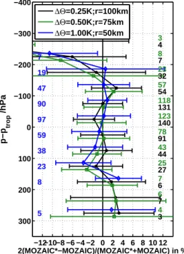
For r < 50 km and 12 < 0.25 K, the small sample size pre-vents drawing concise conclusions, since outliers are heav-ily weighted in the RMSE calculation. Optimal matching criteria are therefore r = 50–100 km and 12 = 0.25–1 K. The comparison is rather robust with respect to the exact match criteria. As shown in Fig. 3, the median of the rela-tive differences as well as the corresponding error bars show a very similar pattern and no statistically significant differ-ence could be identified at the 10 % level (90 % confiddiffer-ence). Match criteria of 12 ≤ ±0.6 K and r ≤ 75 km are chosen for the comparison of aircraft and ozonesondes. Furthermore, we also dismiss all matched trajectories where the weighted (Eq. 2) standard deviation of the matches along a trajectory is ≥ 10 %. We attribute such large variability to either mixing
−12−10−8 −6 −4 −2 0 2 4 6 8 10 12 −400 −300 −200 −100 0 100 200 300 p−p trop /hPa 2(MOZAIC*−MOZAIC)/(MOZAIC*+MOZAIC) in % 3 7 6 27 44 91 140 131 54 32 7 4 4 6 7 25 43 78 123 118 57 23 8 3 5 8 23 38 59 97 90 47 19 7 ∆Θ=0.25K;r=100km ∆Θ=0.50K;r=75km ∆Θ=1.00K;r=50km
Fig. 3. Quality of MOZAIC self-matches depending on match criteria. Differences are grouped into
50hPa bins from the tropopause pressure at 2 PVU obtained at initialization of the trajectories. The hor-izontal bars show the 90 % confidence interval of the median of the relative differences. Numbers denote the number of matched trajectories per bin. MOZAIC* denotes the ozone concentration at initialization of the trajectories. Symbols are slightly shifted to prevent overlap.
28
Fig. 3. Quality of MOZAIC self-matches depending on match
cri-teria. Differences are grouped into 50 hPa bins from the tropopause pressure at 2 PVU obtained at initialization of the trajectories. The horizontal bars show the 90 % confidence interval of the median of the relative differences. Numbers denote the number of matched trajectories per bin. MOZAIC* denotes the ozone concentration at initialization of the trajectories. Symbols are slightly shifted to pre-vent overlap.
along the trajectory, errors in their locations or ozone lami-nae in the profile that remain unresolved in the 1 min aircraft observations. Using these criteria excludes around 6 % of the matched trajectories from the statistical analysis.
3.3 Testing consistency of trajectory matches
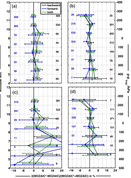
Figure 4a and b reports the results of a self-matching test for 6 day trajectories launched in January, April, July and Oc-tober 2000 and from January to December 2001 as function of altitude and scaled to the tropopause. Since the height of the thermal tropopause cannot be calculated from MOZAIC aircraft observations, we apply a dynamical definition of the tropopause at 2 PVU (potential vorticity unit, 1 PVU = 10−6m2s−1K kg−1, obtained from ERA-Interim fields). In
addition to data for the year 2001, four months from 2000 are used to represent all four seasons and to increase sample size. The error bars in Fig. 4a encompass the 0 % line at all altitude layers, except in the middle troposphere, where the number of matches was small. The vast majority of matched tra-jectories originate between 10–12 km altitude, i.e. at cruise level in the mid-latitudes. Below 10 km altitude the sample size is much smaller. Above 10 km, the mean of the rela-tive differences is around 0 %, however, in contrast, below
Fig. 4. Upper panels (a and b): Sensitivity analysis of self-matching results based on 6 day trajectories
for MOZAIC observations. Difference using only backward trajectories (black), difference using only
forward trajectories (blue) and combination of both, forward- and backward trajectories (green).
Dif-ferences are grouped in 1
km wide altitude layers (a). Differences grouped in 100 hPa bins from the
tropopause pressure at 2 PVU (b). Horizontal bars indicate the 90 % confidence interval of the median
of the relative differences. Black and blue numbers show the number of matched backward and forward
trajectories per bin, respectively. MOZAIC* denotes the ozone concentration at initialization of the
tra-jectories. Symbols are shifted to prevent overlap. Lower panels (c and d): same as in (a) and (b), but
excluding matches from the first 24
h of each trajectory.
29
Fig. 4. Upper panels (a and b): Sensitivity analysis of self-matching results based on 6 day trajectories for MOZAIC observations. Difference
using only backward trajectories (black), difference using only forward trajectories (blue) and combination of both, forward- and backward trajectories (green). Differences are grouped in 1 km wide altitude layers (a). Differences grouped in 100 hPa bins from the tropopause pressure at 2 PVU (b). Horizontal bars indicate the 90 % confidence interval of the median of the relative differences. Black and blue numbers show the number of matched backward and forward trajectories per bin, respectively. MOZAIC* denotes the ozone concentration at initialization of the trajectories. Symbols are shifted to prevent overlap. Lower panels (c and d): same as in (a) and (b), but excluding matches from the first 24 h of each trajectory.
10 km, the mean relative differences range between 2–4 %. These noisier levels may be attributable to the higher sensi-tivity of the match criteria lower down in the troposphere, to the smaller sample size and to lower ozone concentrations. There are small differences between the application of for-ward and backfor-ward trajectories, which are on the order of 2–8 % at lower levels below 10 km altitude, but which are statistically insignificant. The bias of one instrument vs. an-other is slightly higher for backward than forward trajecto-ries, possibly indicating that ozone production occurs in the sampled air masses.
For both forward and backward trajectories, the mean time between a match and the starting point of a trajectory is 1 1/2 days. This time is shorter than for matches with most sounding sites. We therefore also check results from self-matching test against the length of the trajectories. Figure 4c and d shows the results after eliminating all matches within the first 24 h of each trajectory. Results are smoother when they are relative to tropopause pressure, since the represen-tation as a function of geometric altitude suffers from hav-ing only very few matches in the lower four bins, and thus a correspondingly large statistical uncertainty. As expected, the exclusion of the first 24 h leads to substantially larger
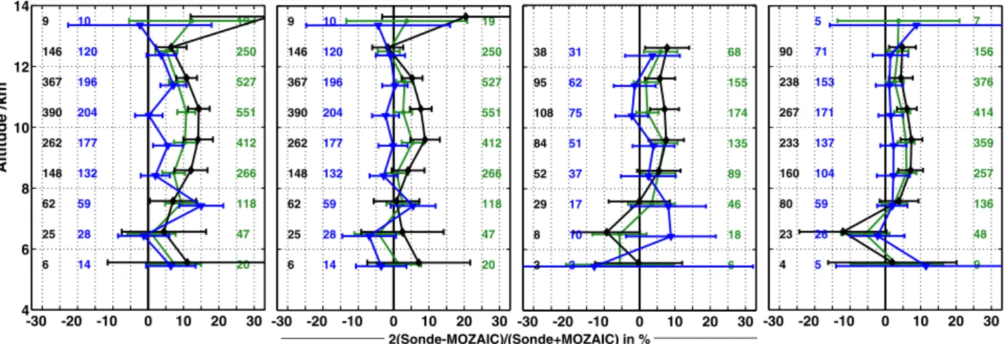
Fig. 5. Median of the relative differences from 6 day trajectories between Payerne ozonesondes and
MOZAIC
O
3measurements averaged over the period 1994–2009. Black: difference using backward
tra-jectories. Blue: difference using forward tratra-jectories. Green: difference using both forward and backward
trajectories. Differences are grouped into 1
km altitude bins. Horizontal bars: 90 % confidence interval
of the median, with number of soundings (N ) per bin. Only data with N > 2 are displayed. The symbols
are slightly shifted vertically for clarity. (First column) Both, BM and ECC profiles are scaled to Arosa
ozone column measurements. (Second column) No column scaling is applied. (Third column) Only 1 day
trajectories are used and sondes not scaled to ozone column. (Fourth column) as for third column but with
four additional trajectories each displaced by 0.5
◦in latitude and longitude from the central trajectory’s
starting position (see text).
30
Fig. 5. Median of the relative differences from 6 day trajectories between Payerne ozonesondes and MOZAIC O3measurements averaged
over the period 1994–2009. Black: difference using backward trajectories. Blue: difference using forward trajectories. Green: difference using both forward and backward trajectories. Differences are grouped into 1 km altitude bins. Horizontal bars: 90 % confidence interval of the median, with number of soundings (N ) per bin. Only data with N > 2 are displayed. The symbols are slightly shifted vertically for clarity. (First column) Both, BM and ECC profiles are scaled to Arosa ozone column measurements. (Second column) No column scaling is applied. (Third column) Only 1 day trajectories are used and sondes not scaled to ozone column. (Fourth column) as for third column but with four additional trajectories each displaced by 0.5◦in latitude and longitude from the central trajectory’s starting position (see text).
error bars at low altitudes (i.e. below 9 km altitude or below 200 hPa from the tropopause) since trajectory errors typically increase with the trajectory length (Stohl, 1998) and because of the significantly reduced sample size. We therefore ex-clude these altitudes by limiting the UTLS to ±125 hPa from the tropopause. This reduces the differences between either including or not including the 24 h to ±3 %. The evidence provided here suggests that three-dimensional trajectories produced using the ERA-Interim reanalysis are suitable for linking different instrumentation platforms to validate ozone measurements. As a result of the larger uncertainty seen in the UTLS when using this technique, a fairly large sample size is required to compensate for statistical errors.
3.4 Comparison of the Payerne ozone soundings with MOZAIC (1994–2009)
The method outlined above allows the determination of av-erage ozone profile differences between the UV photome-ter technique employed by MOZAIC and the routinely flown ozonesondes at Payerne. It also allows a comprehensive anal-ysis of the performance of the ozonesondes over different pe-riods, including changes in sensor types, and an evaluation of the influence of different data processing methods.
The overall mean differences for 1994–2009 are presented in Fig. 5 as a function of sounding altitude at initialization of the trajectories. In total, 1220 soundings can be compared with MOZAIC, i.e. 55 % of the 2247 sondes launched at Pay-erne between August 1994 and March 2009. Most matches are obtained from trajectories that originate between altitudes of 8–12 km. Figure 6 shows the spatial distribution of the matches for Payerne summed up over a 3◦×3◦ grid, with
Fig. 6. Spatial distribution of matches of MOZAIC aircraft observations with (a) backward trajectories and (b) forward trajectories initialized at Payerne. The color bar shows the total number of matches summed up over a3◦× 3◦grid.
31
Fig. 6. Spatial distribution of matches of MOZAIC aircraft
obser-vations with (a) backward trajectories and (b) forward trajectories initialized at Payerne. The colour bar shows the total number of matches summed up over a 3◦×3◦grid.
most matches found over Western and Central Europe. This feature is also reflected in the temporal distribution of the matches, with the majority of matches occurring within the first two days. The geographical distribution of forward and backward trajectory matches differs. The highest number of matches, however, lie to the west of Switzerland for both for-ward and backfor-ward trajectories.
On average, the soundings measure 10 % higher ozone mixing ratios than the UV photometers employed by MOZAIC. This value could be reduced to 5 % if the scal-ing of the whole profile to the Arosa ozone column was not applied (Fig. 5). The differences between forward and back-ward trajectories are 5–10 %, which is substantially higher than expected from the MOZAIC self-matching test. The ozonesondes are significantly higher compared to MOZAIC
(a) (b)
Fig. 7. Sensitivity of relativeO3differences with respect to trajectory starting position. Line style shows
position (see insert). (a) Differences in∆O3when either only forward (∆O3 F
) or only backward tra-jectories (∆O3
B
) are used. (b) Mean deviations between sonde and MOZAIC using both forward and backward trajectories.
32
Fig. 7. Sensitivity of relative O3differences with respect to
trajec-tory starting position. Line style shows position (see insert). (a) Dif-ferences in 1O3when either only forward (1O3F) or only
back-ward trajectories (1O3B) are used. (b) Mean deviations between sonde and MOZAIC using both forward and backward trajectories.
when just back trajectories are used, suggesting that O3 is
produced along the trajectories, and thus violating the as-sumption of O3 being a passive tracer. However, an offset,
although less, is still present in case of 1 day trajectories, a period with much reduced O3production (Fig. 5c).
3.4.1 Sensitivity analysis
Wind speed and direction are not always available at every pressure level for each sounding and thus the reconstructed path of the balloon ascent path may not necessarily be cor-rect. The starting positions of the trajectories may therefore be poorly defined, or possibly wrong in space and/or time. In addition, the spatio-temporal interpolation from the regu-lar numerical model grid to the actual trajectory position can also be critical for complex flows (Stohl et al., 1995). Hence, as sensitivity analysis, four additional trajectories are calcu-lated for every trajectory starting position, each displaced by 0.5◦ latitude and longitude from the central trajectory’s starting position. We initialize these surrounding trajectories with the same O3 concentrations as the central trajectory.
The sensitivity to the different trajectory starting positions in terms of differences in 1O3obtained from backward-only
and forward-only trajectories is shown in Fig. 7a. Although the differences in 1O3between the unidirectional
trajecto-ries amount to 10 % in particular altitude bins (Fig. 7a), the results using combined trajectories are very robust and give similar 1O3 profiles (Fig. 7b). Below 9 km the results are
more sensitive to the starting positions as a result of both the smaller ozone concentrations and smaller sample size in the troposphere, in particular below 7 km. Furthermore, the re-sults from the combined method are hardly affected by the
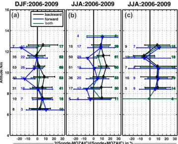
Fig. 8. Similar to Fig. 5. Results for 2006–2009 are plotted using 6 day trajectories for (a) DJF and (b) JJA, as well as using 1 day trajectories for (c) JJA. Sonde profiles are scaled to an independent ozone column.
33
Fig. 8. Similar to Fig. 5. Results for 2006–2009 are plotted using
6 day trajectories for (a) DJF and (b) JJA, as well as using 1 day trajectories for (c) JJA. Sonde profiles are scaled to an independent ozone column.
use of either 1 day or 6 day trajectories (Fig. 5d) emphasis-ing its robustness with respect to the length of the trajecto-ries. For the rest of this analysis we use all trajectories (the central point plus the four displaced trajectories) because of the robust results of combined trajectories, the better agree-ment between forward and backward trajectories in both the 1 day and the 6 day case, and the larger sample size. The sample size now comprises 1899 sondes, 83 % of the sondes launched at Payerne during MOZAIC’s operational phase (1994–2009).
Figure 8 shows 1O3 profiles as a function of altitude
for winter and summer averaged over the period 2006– 2009. Backward trajectories systematically indicate that the ozonesondes have a higher bias to MOZAIC for both sea-sons, typically on the order of 5 %. For most bins the dif-ferences are, however, statistically insignificant. The largest offset between forward and backward trajectory directions is obtained in summer, and is also more pronounced at lower altitudes (reaching up to 15–20 %). This is qualitatively con-sistent with tropospheric summer smog chemistry along the 6 day trajectories in the troposphere, since the 1 day trajec-tories do not show a large offset between the two directions (Fig. 8c). The differences are, however, too large to be ex-plained solely by photochemistry, given the rates of ozone photochemistry in the troposphere. In addition, other fac-tors such as when and where the measurements take place (e.g. before or after a frontal zone, after/before a trough/high) also likely contribute to the observed differences.
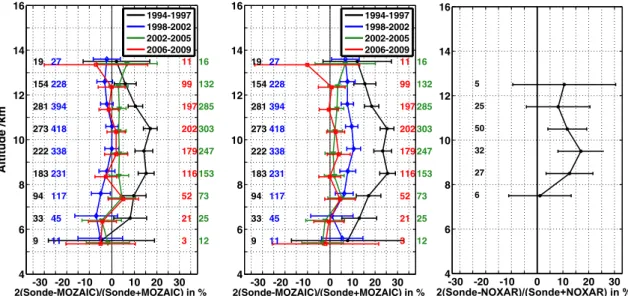
Fig. 9. As for Fig. 5 but results are separated for 4 different periods. Only BM sondes were used for
the periods 1994–1997 and 1998–2002, whereas only ECC sondes were launched during the two later
periods (2002–2006 and 2006–2009). BM and ECC sondes before normalization (left panel). Normalized
BM and ECC sondes (center panel). Median of the relative differences between scaled BM sondes and
NOXAR
O
3measurements averaged over the period 1995–1997 (right panel).
34
Fig. 9. As for Fig. 5 but results are separated for 4 different periods. Only BM sondes were used for the periods 1994–1997 and 1998–
2002, whereas only ECC sondes were launched during the two later periods (2002–2006 and 2006–2009). BM and ECC sondes before normalization (left panel). Normalized BM and ECC sondes (centre panel). Median of the relative differences between scaled BM sondes and NOXAR O3measurements averaged over the period 1995–1997 (right panel).
3.4.2 Analysis of the time series
Figure 9 shows the average difference profile for four differ-ent periods using the combined forward and backward tra-jectories data set: two periods before changing from BM to ECC sondes and two periods after the change. Before 1998, BM sondes exceed MOZAIC up to 25 %, or up to 15 % if data are not scaled to the Arosa column ozone. The expla-nation for this offset is still unclear. Schnadt Poberaj et al. (2009) and Logan et al. (2012) report similar deviations in the 1990s for European BM sondes in the free and upper troposphere. After 1998, however, this large offset is signif-icantly reduced with BM sondes underestimating MOZAIC by < 5 %, if not normalized. Scaling to column ozone can correct for the very low bias, but the mean differences in-crease to 5–10 %. The fact that scaling of BM sondes changes the sign of the bias has also been noted by De Backer et al. (1998) and Stübi et al. (2008). De Backer et al. (1998) also proposed an alternative normalization procedure, which was evaluated by Lemoine and De Backer (2001) against SAGE-II data. Generally, the scaling has been introduced to cor-rect for the low bias of the BM sondes’ column, but this clearly has a strong impact on UTLS ozone measurements. BM-ECC dual flights at Payerne during the OZEX campaign (Stübi et al., 2008) showed that (unscaled) BM sondes under-estimate ozone compared to ECC sondes by approximately 5–8 % in the UTLS, and by 12–15 % in the stratosphere (15– 25 km). Since a single scaling factor, which depends primar-ily on the stratospheric ozone content, is applied to the whole profile, the higher bias of the BM sondes in the stratosphere is carried over into the UTLS. Thus, if scaling is applied to BM
sondes, some portion of 1O3certainly arises from higher
bi-ases of the BM sondes in the stratosphere. The differences in the 1O3 between 1994–1998 and 1998–2002, however,
cannot be explained by the scaling, which is around 1.10 for both periods.
The ECC mean difference profiles between the two pe-riods are rather similar, both showing mean deviations < 5 % (ECC overestimate MOZAIC), in accordance with the JOSIE results (Smit et al., 2007). The normalization does not strongly affect the ECC performance since the correction fac-tor typically is around 1.0.
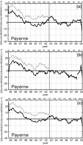
The time series of relative differences are plotted in Fig. 10 for both normalized data and unnormalized data, respec-tively. For each sounding we calculate the mean relative dif-ference per 1 km bin and average over all bins to produce monthly means. Finally, a 13 month central moving average is applied to smooth the time series. In general, the time series’ reproduce the above findings: there is a large offset between BM sondes and MOZAIC’s UV-photometers prior to 1997/1998, which then decreases to < ±10 % after this date, while the mean ECC sonde deviations typically drift around the 0 % line (Fig. 10c). The backward trajectories re-veal a typical positive offset of below 5 %, except for 2006 when the sondes underestimate MOZAIC by 5 %. The dip in 2006 is more pronounced using forward-only trajectories and continues into 2008.
3.5 Comparison of the Payerne soundings with NOXAR measurements
The reason for the large offset between BM sondes and MOZAIC prior to 1997/1998 remains unexplained.
Fig. 10. Times series of the relative differences between sondes and MOZAIC averaged from 4–14
km
altitude, using (a) only backward trajectories, (b) only forward trajectories and (c) combining forward
and backward trajectories. Numbers at the top denote the number of soundings available per year. Gray
lines indicate both BM and ECC sondes scaled. The vertical black solid line denote the change from BM
to ECC sondes in September 2002.
35
Fig. 10. Times series of the relative differences between sondes and
MOZAIC averaged from 4–14 km altitude, using (a) only backward trajectories, (b) only forward trajectories and (c) combining forward and backward trajectories. Numbers at the top denote the number of soundings available per year. Gray lines indicate both BM and ECC sondes scaled. The vertical black solid line denote the change from BM to ECC sondes in September 2002.
Logan et al. (2012), however, found an increase in the MOZAIC bias from 1994–2009 over Frankfurt/Munich com-pared with the alpine surface site Zugspitze. To investigate this further, we assume NOXAR measurements as a ref-erence dataset. We use the same method for comparing BM sondes at Payerne with NOXAR as we used for the MOZAIC comparison. Figure 9c shows that the mean devia-tion between sonde (scaled to column ozone) and NOXAR are around 10–15 %, 5 % lower than the comparison with MOZAIC. The fact that some different ozonesondes are pos-sibly included in the NOXAR comparison should not affect the comparability. However, because of the much smaller sample size, the sonde-NOXAR comparison has much larger uncertainties. The analysis comprises 56 soundings in 1995, 30 in 1996 and only 8 in 1997. Despite the large uncertainty, this somewhat surprising results may indicates that the large offset between MOZAIC and BM sondes prior to 1998 may
possibly be partially attributable to a drift in the MOZAIC calibration. The results seem to be qualitatively consistent with Logan et al. (2012). However, a large part of the tem-poral change in the difference between BM ozonesondes and MOZAIC remains. Note, Dias-Lalcaca et al. (1998) reported an excellent agreement between MOZAIC and NOXAR based on a quasi-simultaneous flight-by-flight comparison. However, their analysis is based on just one simple flight and therefore lacks representativeness.
4 Summary and conclusions
In this paper, we test the application of trajectories for com-paring different ozone measurement platforms in the up-per troposphere/lower stratosphere, such as electrochemical ozonesondes and MOZAIC aircraft observations. Trajecto-ries are driven by ERA-Interim reanalysis wind-fields, en-suring that the model used has not undergone changes in resolution or parameterizations over the period considered, August 1994 to March 2009.
By comparing MOZAIC with MOZAIC (“self-matching”), we found that the trajectory method produces reasonable results showing mean differences of ±2 % between different aircraft, which is considered accurate enough for our purposes. Uncertainties associated with individual trajectories are larger in the UTLS than in the stratosphere, thus, for reliable comparison larger sample sizes are required. Small differences between the results from backward-only and forward-only trajectories provide an indication of the uncertainty associated with this tech-nique, especially when applied to a station close to the Alps, and the difficulties models and trajectories have to accurately quantify the meteorological conditions in the UTLS. The assumption of O3being a passive tracer along the duration of
12 days is critical, especially in the troposphere in summer. Application of the match technique to Payerne ozonesonde data show encouraging agreement with MOZAIC aircraft ob-servations after 1998. The mean differences of ECC sonde type are less than ±5 %, independent of scaling. The BM sondes record from 1998–2002 shows a similar bias but if scaling to total ozone is applied this increases to up to 10 %. Concerning the homogeneity of the time series with respect to MOZAIC, the forward-only case shows that BM sondes agree with the ECC sondes when they are not scaled to col-umn ozone. The pattern obtained from the backward-only case is more difficult to interpret since the ECC sonde dif-ferences amount to 10 % in the first years of operation. In general, however, the homogeneity of the times series seems to be better preserved if no scaling is applied which is differ-ent to findings of Stübi et al. (2008) who recommend scaling both sonde types.
Recently Logan et al. (2012) reported that BM sondes only produced reliable measurements in the troposphere after 1998. When we use NOXAR instead of MOZAIC
measurements, mean differences between sonde and aircraft are roughly 5 % smaller over the 1995–1997 period. This suggests a possible drift in the MOZAIC calibration, consis-tent with the findings of Logan et al. (2012). This drift, how-ever, cannot entirely explain the large differences between sonde and MOZAIC observations observed before 1998.
Payerne was chosen as a test site for this method since it is a very well documented sounding station and we could confirm our results with previous publications. In a com-panion paper (Staufer et al., 2013), results from many other ozonesonde stations are discussed. Sites include Sodankylä (Northern Finland) and Scoresbysund (Greenland), both of which are far away from any MOZAIC airport and thus tra-jectories are essential to compare the different observation platforms. We aim to provide a coherent overview of the performance of the various ozonesonde sites and to evaluate the reliability and consistency of their records in the UTLS which is vital because different sonde types, sensors, prepa-ration and processing procedures have been used and/or have changed.
Acknowledgements. J. Staufer’s search was funded by a
Me-teoSwiss GAW-CH grant. The authors warmly acknowledge the European Commission, Airbus, CNRS-France, and FZJ-Germany for their strong support of the MOZAIC project and the airlines (Lufthansa, AirFrance, Austrian, Air Namibia, and former Sabena) who have carried the MOZAIC instrumentation free of charge since 1994. MOZAIC is presently funded by INSU-CNRS (France), Météo-France, CNES, Université Paul Sabatier (Toulouse, France) and Research Center Jülich (FZJ, Jülich, Germany). IAGOS is ad-ditionally funded by the EU projects IAGOS-DS, IAGOS-ERI, and IGAS. MOZAIC-IAGOS data are available via the CNES/CNRS-INSU Ether web-site http://www.pole-ether.fr. Ozonesonde data used in this publication were obtained from the World Ozone and Ultraviolet Radiation Data Center (WOUDC, located in Toronto and operated by Environment Canada; publicly available at http://www.woudc.org) and were downloaded between March and April 2010. We are grateful to the soundings team at Payerne, who carefully prepare and perform all the launches. Finally, thanks are also due to Swiss International Air Lines, successor of SwissAir, for fruitful collaboration within the NOXAR project.
Edited by: S. Godin-Beekmann
References
Bodeker, G. E., Boyd, I. S., and Matthews, W. A.: Trends and vari-ability in vertical ozone and temperature profiles measured by ozonesondes at Lauder, New Zealand: 1986–1996, J. Geophys. Res., 103, 28661–28681, 1998.
Brewer, A. and Milford, J.: The Oxford Kew ozonesonde, P. Roy. Soc. Lond., 256, 470–495, doi:10.1098/rspa.1960.0120, 1960. Brunner, D., Staehlin, J., Jeker, D., Wernli, H., and Schumann, U.:
Nitrogen oxides and ozone in the tropopause region of the Northern Hemisphere: measurements from commercial aircraft
in 1995/1996 and 1997, J. Geophys. Res., 106, 27673–27699, 2001.
Brunner, D., Staehelin, J., Rogers, H. L., Köhler, M. O., Pyle, J. A., Hauglustaine, D., Jourdain, L., Berntsen, T. K., Gauss, M., Isak-sen, I. S. A., Meijer, E., van Velthoven, P., Pitari, G., Mancini, E., Grewe, G., and Sausen, R.: An evaluation of the performance of chemistry transport models by comparison with research air-craft observations – Part 1: Concepts and overall model perfor-mance, Atmos. Chem. Phys., 3, 1609–1631, doi:10.5194/acp-3-1609-2003, 2003.
Claude, H., Hartmannsgruber, R., and Köhler, U.: Measurement of Atmospheric Ozone Profiles Using the Brewer/Mast Sonde – Preparation, Procedure, Evaluation, WMO Global Ozone Re-search and Monitoring Project, 17, World Meteorol. Organ., Geneva, Switzerland, 1987.
Cui, J., Sprenger, M., Staehelin, J., Siegrist, A., Kunz, M., Henne, S., and Steinbacher, M.: Impact of stratospheric intru-sions and intercontinental transport on ozone at Jungfraujoch in 2005: comparison and validation of two Lagrangian approaches, Atmos. Chem. Phys., 9, 3371–3383, doi:10.5194/acp-9-3371-2009, 2009.
Danilin, M. Y., Santee, M. L., Rodriguez, J. M., Ko, M. K. W., Mer-genthaler, J. M., Kumer, J. B., Tabazadeh, A., and Livesey, N. J.: Trajectory hunting: a case study of rapid chlorine activation in December 1992 as seen by UARS, J. Geophys. Res., 105, 4003– 4018, 2000.
Danilin, M. Y., Ko, K. W., Bevilacqua, R. M., Lyjak, L. V., Froidevaux, L., Santee, M. L., Zawodny, J. M., Hoppel, K. W., Richard, E. C., Spackman, J. R., Weinstock, E. M., Her-man, R. L., McKinney, K. A., Wennberg, P. O., Eisele, F. L., Stimpfle, R. M., Scott, C. J., Elkins, J. W., and Bui, T. V.: Com-parison of ER-2 aircraft and POAM III, MLS, and SAGE II satel-lite measurements during SOLVE using traditional correlative analysis and trajectory hunting technique, J. Geophys. Res., 107, 8315, doi:10.1029/2001JD000781, 2002a.
Danilin, M. Y., Ko, M. K. W., Froidevaux, L., Santee, M. L., Ly-jak, L. V., Bevilacqua, R. M., Zawodny, J. M., Sasano, Y., Irie, H., Kondo, Y., Russell III, J. M., Scott, C. J., and Read, W. G.: Tra-jectory Hunting as an effective technique to validate multiplat-form measurements: analysis of the MLS, HALOE, SAGE-II, ILAS and POAM-II data in October–November 1996, J. Geo-phys. Res., 107, 4420, doi:10.1029/2001JD002012, 2002b. De Backer, H., De Muer, D., and De Sadelaer, G.: Comparison
of ozone profiles obtained with Brewer–Mast and Z-ECC sen-sors during simultaneous ascents, J. Geophys. Res., 103, 19641– 19648, 1998.
Dias-Lalcaca, P., Brunner, D., Imfeld, W., Moser, W., and Staehe-lin, J.: An automated system for the measurement of nitrogen oxides and ozone concentrations from a passenger aircraft: in-strumentation and first results of the project NOXAR, Environ. Sci. Technol., 32, 3228–3236, 1998.
Forster, P. M. D. F. and Shine, K. P.: Radiative forcing and temper-ature trends from stratospheric ozone changes, J. Geophys. Res., 102, 10841–10855, 1997.
Hegglin, M. I. and Shepherd, T. G.: Large climate-induced changes in ultraviolet index and stratosphere-to-troposphere ozone flux, Nat. Geosci., 2, 687–691, 2009.
Hilsenrath, E. W., Attmannspacher, W., Bass, A., Evans, W., Hagemeyer, R., Barnes, R. A., Komhyr, W., Mauersberger, K.,
Mentall, J., Proffitt, M., Robbins, D., Taylor, S., Torres, A., and Weinstock, E.: Results from the balloon ozone intercomparison campaign (BOIC), J. Geophys. Res., 91, 13137–13152, 1986. Jeannet, P., Stübi, R., Levrat, G., and Staehelin, J.: Ozone
bal-loon soundings at Payerne (Switzerland): reevaluation of the time series 1967–2002 and trend analysis, J. Geophys. Res., 112, D11302, doi:10.1029/2005JD006862, 2007.
Komhyr, W. D.: Electrochemical concentration cells for gas analy-sis, Ann. Geophys., 25, 203–210, 1969,
http://www.ann-geophys.net/25/203/1969/.
Komhyr, W. D., Barnes, R. A., Brothers, G. B., Lathrop, J. A., and Opperman, D. P.: Electrochemical concentration cell ozonesonde performance evaluation during STOIC 1989, J. Geophys. Res., 100, 9231–9244, 1995.
Labow, G. J., McPeters, R. D., Bhartia, P. K., and Kramarova, N.: A comparison of 40 years of SBUV measurements of column ozone with data from the Dobson/Brewer network, J. Geophys. Res. Atmos., 118, 7370–7378, doi:10.1002/jgrd.50503, 2013. Lacis, A. A., Wuebbles, D. J., and Logan, J. A.: Radiative forcing of
climate by changes in the vertical distribution of ozone, J. Geo-phys. Res., 95, 9971–9981, 1990.
Law, K. S., Plantevin, P.-H., Thouret, V., Marenco, A., As-man, W. A. H., Lawrence, M., Crutzen, P. J., Muller, J.-F., Hauglustaine, D. A., and Kanakidou, M.: Comparison be-tween global chemistry transport model results and Measure-ments of Ozone and Water Vapor by Airbus In-Service Aircraft (MOZAIC) data, J. Geophys. Res., 105, 1503–1525, 2000. Lemoine, R. and De Backer, H.: Assessment of the Uccle ozone
sounding time series quality using SAGE II data, J. Geophys. Res., 106, 14515–14523, doi:10.1029/2001JD900122, 2001. Liu, S. C., Trainer, M., Fehsenfeld, F. C., Parrish, D. D.,
Williams, E. J., Fahey, D. W., Hübler, G., and Murphy, P. C.: Ozone production in the rural troposphere and the implications for regional and global ozone distributions, J. Geophys. Res., 92, 4191–4207, 1987.
Liu, X., Chance, K., Sioris, C. E., Kurosu, T. P., and Newchurch, M. J.: Intercomparison of GOME, ozonesondes, and SAGE II measurements of ozone: demonstration of the need to homogenize available ozonesonde data sets, J. Geophys. Res., 111, D14305, doi:10.1029/2005JD006718, 2006.
Logan, J. A., Megretskaia, I. A., Miller, A. J., Tiao, G. C., Choi, D., Zhang, L., Stolarski, R. S., Labow, G. J., Hollandsworth, S. M., Bodeker, G. E., Claude, H., De Muer, D., Kerr, J. B., Tara-sick, D. W., Oltmans, S. J., Johnson, B., Schmidlin, F., Staehe-lin, J., Viatte, P., and Uchino, O.: Trends in the vertical distribu-tion of ozone: a comparison of two analysis of ozonesonde data, J. Geophys. Res., 104, 26373–26399, 1999.
Logan, J. A., Staehelin, J., Megretskaia, I. A., Cammas, J.-P., Thouret, V., Claude, H., De Backer, H., Steinbacher, M., Scheel, H.-E., Stübi, R., Fröhlich, M., and Derwent, R.: Changes in ozone over Europe: analysis of ozone measurements from son-des, regular aircraft (MOZAIC) and alpine surface sites, J. Geo-phys. Res., 117, D09301, doi:10.1029/2011JD016952, 2012. Marenco, A., Thouret, V., Nédélec, P., Helten, M., Kley, D.,
Karcher, F., Simon, P., Law, K., Pyle, J., Poschmann, G., Von Wrede, R., Hume, C., and Cook, T.: Measurement of ozone and water vapour by Airbus in-service aircraft: the MOZAIC airborne program, an overview, J. Geophys. Res., 103, 25631– 25642, 1998.
Morris, G. A., Gleason, J. F., Ziemke, J., and Schoeberl, M. R.: Tra-jectory mapping: a tool for validation of trace gas observations, J. Geophys. Res., 105, 17875–17894, 2000.
Morris, G. A., Bojkov, B. R., Lait, L. R., and Schoeberl, M. R.: A review of the Match technique as applied to AASE-2/EASOE and SOLVE/THESEO 2000, Atmos. Chem. Phys., 5, 2571–2592, doi:10.5194/acp-5-2571-2005, 2005.
Rex, M., von der Gathen, P., Harris, N. R. P., Lucic, D., Knud-sen, B. M., Braathen, G. O., Reid, S. J., De Backer, H., Claude, H., Fabian, R., Fast, H., Gil, M., Kyrö, E., Mikkelsen, I. S., Rummukainen, M., Smit, H. G., Stähelin, J., Varotsos, C., and Zaitcev, I.: In situ measurements of strato-spheric ozone depletion rates in the Arctic winter 1991/1992: a Lagrangian approach, J. Geophys. Res., 103, 5843–5853, 1998. Schnadt Poberaj, C., Staehelin, J., Brunner, D., Thouret, V., De Backer, H., and Stübi, R.: Long-term changes in UT/LS ozone between the late 1970s and the 1990s deduced from the GASP and MOZAIC aircraft programs and from ozonesondes, Atmos. Chem. Phys., 9, 5343–5369, doi:10.5194/acp-9-5343-2009, 2009.
Shepherd, T. G.: Dynamics, stratospheric ozone, and climate change, Atmos. Ocean, 46, 117–138, doi:10.3137/ao.460106, 2008.
Smit, H. G. J.: Ozonesondes, in: Encyclopedia of Atmospheric Sci-ences, edited by: Holton, J., Pyle, J., and Curry, J., Academic Press, London, 1469–1476, 2002.
Smit, H. G. J. and Kley, D.: JOSIE: the 1996 WMO international intercomparison of ozonesondes under quasi flight conditions in the environmental simulation chamber at Jülich, WMO Global Atmos. Watch Rep., 130, World Meteorol. Organ., Geneva, Switzerland, 1998.
Smit, H. G. J. and Straeter, W.: JOSIE-1998, Performance of ECC Ozone Sondes of SPC-6A and ENSCI-Z Type, WMO Global Atmos. Watch Rep., 157, World Meteorol. Organ., Geneva, Switzerland, 2004a.
Smit, H. G. J. and Straeter, W.: JOSIE-2000, Jülich Ozone Sonde Intercomparison Experiment 2000, the 2000 WMO international intercomparison of operating procedures for ECC-ozonesondes at the environmental simulation facility at Jülich, WMO Global Atmos. Watch Rep., 158, World Meteorol. Organ., Geneva, Switzerland, 2004b.
Smit, H. G. J., Sträter, W., Helten, M., and Kley, D.: Environmental simulation facility to calibrate airborne ozone and humidity sen-sors, Jül-Berichte, 3796, Forschungszentrum Jülich, Jülich, Ger-many, 2000.
Smit, H. G. J., Straeter, W., Johnson, B. J., Oltmans, S. J., Davies, J., Tarasick, D. W., Hoegger, B., Stubi, R., Schmidlin, F. J., Northam, T., Thompson, A. M., Witte, J. C., Boyd, I., and Posny, F.: Assessment of the performance of ECC-ozonesondes under quasi-flight conditions in the environmental simulation chamber: insights from the Juelich Ozone Sonde Intercom-parison Experiment (JOSIE), J. Geophys. Res., 112, D19306, doi:10.1029/2006JD007308, 2007.
SPARC/IOC/GAW: Assessment of Trends in the Vertical Distribu-tion of Ozone, edited by: Harris, N., Hudson, R., and Phillips, C., SPARC Report No. 1, WMO Ozone Research and Monitoring Project, Report 43, WMO, World Meteorol. Organ., Geneva, Switzerland, 1998.
Staufer, J., Staehelin, J., Stübi, R., Peter, T., Tummon, F., and Thouret, V.: Trajectory matching of ozonesondes and MOZAIC measurements in the UTLS – Part 2: Application to the global ozonesonde network, Atmos. Meas. Tech. Discuss., 6, 7099– 7148, doi:10.5194/amtd-6-7099-2013, 2013.
Stohl, A.: Computation, accuracy and applications of trajectories – a review and bibliography, Atmos. Environ., 32, 947–966, 1998. Stohl, A.: A 1-year Lagrangian “climatology” of airstreams in the Northern Hemisphere troposphere and lowermost stratosphere, J. Geophys. Res., 106, 7263–7279, 2001.
Stohl, A., Wotawa, G., Seibert, P., and Kromp-Kolb, H.: Interpola-tion errors in wind fields as a funcInterpola-tion of spatial and temporal resolution and their impact on different types of kinematic tra-jectories, J. Appl. Meteorol., 34, 2149–2165, 1995.
Stübi, R., Levrat, G., Hoegger, B., Viatte, P., Staehelin, J., and Schmidlin, F. J.: In-flight comparison of Brewer–Mast and elec-trochemical concentration cell ozonesondes, J. Geophys. Res., 113, D13302, doi:10.1029/2007JD009091, 2008.
Tarasick, D. W., Fioletov, V. E., Wardle, D. I., Kerr, J. B., and Davies, J.: Changes in the vertical distribution of ozone over Canada from ozonesondes: 1980–2001, J. Geophys. Res., 140, D02304, doi:10.1029/2004JD004643, 2005.
Thouret, V., Marenco, A., Logan, J. A., Nédélec, P., and Grouhel, C.: Comparisons of ozone measurements from the MOZAIC airborne program and the ozone sounding network at eight locations, J. Geophys. Res, 103, 25695–25720, 1998a.
Thouret, V., Marenco, A., Nédélec, P., and Grouhel, C.: Ozone cli-matologies at 9–12 km altitude as seen by the MOZAIC airborne program between September 1994 and August 1996, J. Geophys. Res, 103, 25653–25679, 1998b.
Thouret, V., Cammas, J.-P., Sauvage, B., Athier, G., Zbinden, R., Nédélec, P., Simon, P., and Karcher, F.: Tropopause referenced ozone climatology and inter-annual variability (1994–2003) from the MOZAIC programme, Atmos. Chem. Phys., 6, 1033–1051, doi:10.5194/acp-6-1033-2006, 2006.
Vömel, H. and Diaz, K.: Ozone sonde cell current measurements and implications for observations of near-zero ozone concentra-tions in the tropical upper troposphere, Atmos. Meas. Tech., 3, 495–505, doi:10.5194/amt-3-495-2010, 2010.
Wernli, H. and Bourqui, M.: A Lagrangion “1-year climatol-ogoy” of (deep) cross-tropopause exchange in the extrat-ropical Northern Hermisphere, J. Geophys. Res., 107, 4021, doi:10.1029/2001JD000812, 2002.
Wernli, H. and Davies, H. C.: A Lagrangian-based analysis of ex-tratropical cyclones. I: The method and some applications, Q. J. Roy. Meteorol. Soc., 123, 467–489, 1997.
World Meteorological Organization: WMO Bulletin, Vol. 6, World Meteorol. Organ., Geneva, Switzerland, 1957.