HAL Id: lirmm-01319093
https://hal-lirmm.ccsd.cnrs.fr/lirmm-01319093
Submitted on 17 Jul 2019
HAL is a multi-disciplinary open access
archive for the deposit and dissemination of
sci-entific research documents, whether they are
pub-lished or not. The documents may come from
teaching and research institutions in France or
abroad, or from public or private research centers.
L’archive ouverte pluridisciplinaire HAL, est
destinée au dépôt et à la diffusion de documents
scientifiques de niveau recherche, publiés ou non,
émanant des établissements d’enseignement et de
recherche français ou étrangers, des laboratoires
publics ou privés.
Collision for Estimating SCA Measurement Quality and
Related Applications
Ibrahima Diop, Mathieu Carbone, Sébastien Ordas, Yanis Linge, Pierre Yvan
Liardet, Philippe Maurine
To cite this version:
Ibrahima Diop, Mathieu Carbone, Sébastien Ordas, Yanis Linge, Pierre Yvan Liardet, et al.. Collision
for Estimating SCA Measurement Quality and Related Applications. CARDIS: Smart Card Research
and Advanced Applications, Nov 2015, Bochum, Germany. pp.143-157,
�10.1007/978-3-319-31271-2_9�. �lirmm-01319093�
Quality and Related Applications
Ibrahima Diop1,4, Mathieu Carbone2, Sebastien Ordas2, Yanis Linge1, Pierre Yvan Liardet1, and Philippe Maurine2,3
1
STMicroelectronics, Rousset
2 LIRMM, Universit´e Montpellier II 3
CEA 880 route de Mimet, 13541 Gardanne
4 Ecole des Mines de Saint-Etienne (EMSE)
Abstract. If the Signal to Noise Ratio (SNR) is a figure of merit com-monly used in many areas to gauge the quality of analogue measure-ments, its use in the context of Side-Channel Attacks (SCA) remains very difficult because the nature and characteristics of the signals are not a priori known. Consequently, the SNR is rarely used in this latter area to gauge the quality of measurements or of experimental protocols followed to acquire them. It is however used to quantify the amount of leakage in a set of traces regardless of the quality of the measures. This is a surprisingly lack despite the key role of measurements and experiments in this field. In this context, this paper introduces a fast and accurate method for estimating the SNR. Then, simple and accurate techniques are derived. They allow to process some daily tasks the evaluators have to perform in a pragmatic and efficient manner. Among them one can find the analysis of the electrical activity of Integrated Circuit (IC) or the identification of the frequencies carrying some information or leakages.
1
Introduction
In recent years, emphasis has been put on the localization of leaking content in space [13], [4], [14] and time [1], but also to increase our understanding of the latest or again to enhance our extraction capability [9], [2], [6]. Efforts have also been invested to assess the efficiency of attacks resulting in notions like the success rate and the guessing entropy.
Based on [16], one generally considers two types of evaluation metrics for assessing the leakage emitted by cryptographic devices. First, information the-oretic metrics aim to capture the amount of information available in a side-channel leakage, independently of the adversary exploitation. Second, security metrics aim to quantify how this information can be exploited by adversary using the notions of Success Rate (SR) and Guessing Entropy (GE). In SCA context, these two types of metrics are clearly related but they are also surrounded by the quality of measurements for which less attention has been paid to define criteria allowing to compare experimental practices that are central.
The Signal-to-Noise Ratio (SNR) is a simple, intuitive and relevant metric to characterize any analog phenomena, such as side channel measurements in order to gauge the quality of acquisition campaign. However the first definition of SNR [10] in the SCA context has some drawbacks making its practical use difficult given that the signal and its characteristics are a priori not known. Some workarounds have been proposed in the literature but most of them rely in converting the problem into leakage quantification or Points of Interest (PoI) detection rather than focusing the quality of the acquisition campaigns. Among these works, one may include the approach proposed in 2011 [7] that offers a method for estimating the SNR which is based on a linear model of the leak-age but also on empirical considerations related to the use of Digital Sampling Oscilloscopes (DSO). However, the SNR definition considered in this work is rel-atively far from the standard electrical engineering definition and finally closer to that of a Leakage to Noise Ratio (LNR) concept.
This latter concept appears explicitly in [17] with an estimation method based on a modeling of the leakage in the frequency domain. Alongside the introduction of the LNR, authors in [1] propose the Normalized Inter-Class Variance (NICV). This approach based on a clever and effective use of the statistical tool of ANOVA (ANalysis Of VAriance) where the F-test allows to identify the PoI thanks to the knowledge of public information (plaintext or ciphertext) (i.e. allows to detect interesting time samples carrying potential leakage based on the manipulation of the inputs). Besides this important application, it is also suggested that the NICV provides an estimate of the SNR. However, again the SNR definition considered in this paper is more an estimate of the relative amount of leakage in the samples of traces that an estimate of the SNR of a measurement set.
In this context, the main contribution of this paper to the State of the Art is a method, based on signal collisions, to estimate the SNR. This method requires a small amount of measures to be applied: two in theory and up to few tens for convenient practice.
The second contribution is to show that this SNR estimate is also an effective way to gauge the quality of traces in view of the application of SCA. Additionally, it is then shown how to exploit the above technique to:
– analyze the temporal behavior of a circuit from a small amount of measures, – distinguish the frequencies carrying information related to the signal from
the frequencies essentially made up of noise.
The distinction of frequencies carrying information is crucial. Indeed, it enables, without any a priori knowledge about the characteristics of the signal, to ratio-nally and adaptively guide the filtering procedures.
This paper is organized as follows: in section 2, the meaning of the term signal considered in this paper, and related SNR is defined. Section 3 recalls the standard electrical engineering definition of the SNR and the corollary defini-tion thereof in the case of zero mean signals. These definidefini-tions recalled, secdefini-tion 4 demonstrates theoretically how to get an estimate of the SNR from signal collisions and more particularly from a bounded collision detection criterion in-troduced in [8]. It is then experimentally demonstrated in section 5 that the
obtained SNR estimate is actually a figure of merit for gauging the quality of traces in a SCA context. Similarly, section 6 shows how this fast estimate method of the SNR allows analyzing SCA traces in a simple, effective and complemen-tary way to the approaches introduced in [1] and [17]. Section 7 shows how to accurately distinguish with a small amount of traces the harmonics of the sig-nal from harmonics mainly related to noise. Fisig-nally, a conclusion is drawn in section 8.
2
Preamble
In this paper, the term signal is devoted to the deterministic evolution (repeated and measured n times with perfect equipments in the absence of any noise source, the signal is unique) of a physical quantity over time, evolving in response to an unique stimulus. For example the evolution of the magnetic field at the co-ordinate (X, Y, Z) above a given IC computing the cipher of a given text with a given key is a signal. The changing of one of these parameters by solely one bit gives a new signal.
In the classical literature such as [11], [1], [10], [17], the power consumption of a measure (trace) is defined as the sum of the exploitable power consumption from an SCA point of view (Pexp), the power of the noise ( considered in [11] as the sum of the electronic noise Pel.noise and of the switching noise Psw.noise) and a constant power consumption (Pconst). In the present paper, we consider the power consumption of a measure as the sum of the power consumptions of the signal (PS) to be measured and of the noise (PN). PS is considered regardless the power consumption of signal is exploitable or not. As a result, PS includes but is not reduced to Pexp. This choice is done in order to evaluate the quality of the measurement protocol independently from the fact that traces contain exploitable information.
None of these meanings is preferable. They are adopted for different pur-poses. In our case, a paradigm shift is investigated to assess the quality of a measurement. This also allows to assess the quality of the related experimental protocol, as an alternative of quantifying the amount of leakage present in a set of SCA traces. However we make a parallel with our approach and this point later in the paper.
3
SNR definition and the related problem
With the definition of the signal adopted in this paper, the SNR is an objective figure of merit for gauging the quality of the measurement M (t) = [m1, ..., mq] of a signal S(t) = [s1, ..., sq], which depends on the surrounding noise, but also of the quality of the equipments used to collect it. The standard electrical engi-neering definition of the SNR is the ratio between the power PS of the signal to be measured and the power PN of noise N (t) = [η1, ..., ηq]:
SN R = PS PN = 1 q · Pq i=1(si)2 1 q· Pq i=1(ηi)2 (1)
If the signal and the noise are zero mean, the numerator and the denominator of Equation 1 are the signal and noise variances, respectively. This leads, consid-ering S(t) and N (t) as random variables over time (horizontal random variables or random processes), to the following compact expression of the SNR:
SN R = σ 2 S σ2 N = 1 q· Pq i=1(si− 0) 2 1 q· Pq i=1(ηi− 0)2 (2)
with σS and σN denoting the standard deviations (measured horizontally and not vertically) of the signal S(t) and noise N (t), respectively. It should be noted that even if the SNR takes the form of a variance ratio, this is really a power ratio and must be perceived as it.
This SNR definition is particularly interesting in the context of SCA exploit-ing the Electro-Magnetic (EM) channel. Indeed, the means of the EM signals are always very close to zero, or can even be fixed to zero by forcing the usual voltage amplifiers to work in small signals or by compensating their input offset voltage. This definition is therefore considered in the rest of this paper. However, given that in the context of SCA, the signal characteristics are not known, this definition is extremely difficult to apply in this form. A solution must therefore be found to extract from measures the SNR values ( Equation 2).
4
From Collisions to SNR estimations
If in the context of SCA the signal S(t) is not known, other degrees of freedom are available to adversaries. One of these degrees of freedom is the capability to stimulate the circuit n times in the same manner to collect n measures of a same execution or calculus. However, this degree of freedom is not unlimited. Indeed, some security protocols limit to few units the possibility to repeat a same execution. In addition, if this is not the case, repeating the same execution is theoretically possible but often tedious because of misalignment of traces which implies the use of some more or less costly realignment techniques. However, it seems possible to generate few colliding traces and exploit them to estimate the SNR as explained below.
4.1 From Bounded Collision Detection Criterion to SNR
The use of signal collisions is a recognized technique to attack the implementa-tions of symmetric [15] or asymmetric [5], [18] algorithms. For this purpose, a choice of plaintexts is done in order to induce a collision between intermediate values according to the targeted secret. The adversary finally derives the secret from the occurrence or the absence of the collision. However, because in practice
SCA traces are noisy, detection is not straightforward and some signal processing techniques are necessary to exploit collisions. Recently in [8], a criterion that au-tomates the detection of collisions was proposed. This criterion, called Bounded Collision Detection Criterion (BCDC), takes values in [0,1] and is defined by:
BCDC(M1, M2) = 1 √ 2 × σ(M1−M2) σ(M1) (3)
where Mi = [mi1, · · · , miq] is a measurement, collected with a Digital Sampling Oscilloscope (DSO), representing a measure of the signal S(t)icharacterized by a (horizontal) standard deviation σ(Mi). The idea behind this criterion is that in
case of collision the numerator is close to zero, while in the absence of collision the BCDC is close to one.
Assuming that all samples mijof these measurements (with j ∈ [1, q]) can be expressed by mi
j = sij+ ηji, i.e. is the sum of: • a deterministic value (si
j) which is a sample of S(t) emitted by the Device Under Test (DUT), at time t, during its operation,
• and of the realization of the noise (ηi
j), which is a random variable, drawn in a normal distribution with zero mean and an unknown standard deviation, it is then possible to express the difference between M1and M2:
∆M = M1− M2= [δm1, · · · , δmq] (4) with δmj = m 1 j− m 2 j = s 1 j+ η 1 j− (s 2 j+ η 2 j). (5)
Considering that all terms of Equation 5 are independent, it appears that the denominator of the BCDC, Equation 3, can be expressed as:
σ(M1−M2)=
q σ2([s1
1− s21, · · · , s1q− s2q]) + σ2([η11− η21, · · · , ηq1− ηq2]), (6) expression that can be re-written:
σ(M1−M2)= q 2 · σ2 S+ 2 · σN2 = √ 2 · q σ2 S+ σ2N (7) Starting from this expression, one can calculate the asymptotic BCDC value when M1 and M2are two measures of the same signal, i.e. in case of a collision. Indeed, in that case, because s1
j = s2j and thus because: σ(M1−M2)= √ 2 · q σ2 N, (8) equation 3 becomes: BCDC(M1, M2) =√1 2 √ 2 · σN pσ2 S+ σ 2 N = q 1 1 + σ2s σ2 N = 1 p1 + SN R(M1, M2) . (9)
As a result, the quick and pragmatic estimate of the SNR becomes possible in the context of SCA. To do this, simply collect n (> 1) traces corresponding to the execution of the same calculus by the DUT; then calculate the 12· n · (n − 1) BCDC values and finally deduce as much values SN R(Mi, Mj):
SN R(Mi, Mj) =
1
BCDC2(Mi, Mj)− 1 (10) Finally, the SNR of a set of traces is estimated by averaging these 1
2· n · (n − 1) SN R(Mi, Mj) values (see Equation 11). In the remainder of the paper this estimation is denoted \SN R. \ SN R = 2 n · (n − 1) n X i=1 n X j=i+1 ( 1 BCDC2(M i, Mj) − 1) (11)
This mean value as well as the shape of the SN R(Mi, Mj) distribution constitute figures of merit for gauging the quality of a SCA measures and that of the experimental protocol that has been followed to collect them: the higher \SN R is, the better the experimental protocol is. As an illustration, typical SN R(Mi, Mj) distributions are given Figure 2c and Figure 2d in section 5. Next paragraphs give an illustration in a school book case.
4.2 Example
To provide practical and convincing elements about the accuracy and the sim-plicity of this fast SNR estimation method, which is applicable when the signal and the data are not known, simulated traces were generated. They relate to the measure of a sinusoidal signal of amplitude equal to 1 and with an horizontal variance over a period of 2 (σS =√2 on a period) in an environment producing a normal measurement noise with zero mean and standard deviation σN.
Table 2 gives the exact SNR value wrt σN as well as \SN R wrt the number of measurements (n = {2, ..., 50}) used to estimate it with the proposed method. One may observe that with only five colliding measures (i.e. 10 BCDC and SN R(Mi, Mj) estimates) \SN Rn=5is really close to the exact SNR value. Indeed, the relative absolute value is lower than 5%. This result appears even more accurate when σSN R is low. For n = 50 measures (i.e. 1275 BCDC values) and for σN = 1.9, \SN Rn=50is equal to 0.1385 and σSN Ris equal to 0.0048 i.e. 3.45% of the exact SNR value. These results demonstrate the practicability as well the accuracy of the proposed method.
4.3 Discussion
At this stage, a fast SNR estimation method to be applied when the signal is not known has been introduced and its accuracy demonstrated. It is based on the SNR definition commonly used to assess the quality of analog measures or
Table 1. Evolution of the mean \SN R value wrt σNand the number n of measurements used to estimate it σN 0.1 0.3 0.5 0.7 0.9 1.1 1.3 1.5 1.7 1.9 SNR 50 5.56 2.00 1.02 0.62 0.41 0.30 0.22 0.17 0.14 \ SN Rn=2 49.38 5.58 2.03 1.00 0.64 0.41 0.28 0.24 0.17 0.16 \ SN Rn=5 49.76 5.51 1.99 1.03 0.60 0.41 0.29 0.21 0.17 0.14 \ SN Rn=10 50.41 5.56 1.99 1.02 0.62 0.41 0.29 0.21 0.18 0.14 \ SN Rn=20 49.91 5.52 2.00 1.03 0.62 0.41 0.30 0.22 0.17 0.14 \ SN Rn=50 50.08 5.56 2.01 1.01 0.62 0.41 0.30 0.22 0.17 0.14
the quality of a communicating channel. This method is the main contribution of this paper.
If the definition considered in this paper is different to that adopted in [10], [11] and [1], in which the authors aim at quantifying the amount of exploitable (with CPA) leakage in set of traces, nothing forbids to assess whether the defini-tion considered in this paper is also an indirect measure of the amount of leakage present in traces. After all, measures of high quality are they not susceptible to convey more leakage than bad quality measurements?
This can be envisaged since the SNR definition adopted in this paper is the ratio between the signal and noise powers, and thus because the signal power is necessarily an upper bound of the exploitable leakage power QL, i.e. the power consumed by the cryptographic operation targeted by the adversary:
σ2S σ2 N ≥σ 2 QL σ2 N ≥ 0 (12)
If the SNR definition considered in this paper is indeed a figure of merit of SCA trace quality, the idea we propose to quantify the quality of a set of SCA traces is simple. It consists in acquiring a small amount of traces (2 to 50 for instance) of a same computational activity (or pairs of the same activity) in order to evaluate \
SN R and if necessary to draw the SN R(Mi, Mj) distribution. This value (or the estimated distribution law) will be considered as a quality measure of SCA traces but also of the experimental protocol applied to collect the traces.
5
Estimated SNR wrt CPA efficiency
To assess if the SNR definition considered in this paper, dedicated to the evalu-ation of the quality of measures and of the experimental protocol used to obtain it, is also an indicator of the amount of leakage in a set traces of SCA and more precisely an upper bound, various experiments were conducted. One challenge was to define an experiment allowing to vary the SNR.
5.1 Experiments
In order to vary the SNR, different experimental campaigns were conducted, and different sets of EM traces, characterized by different SNR values were collected. These campaigns have consisted in measuring the EM radiations of an AES mapped into an FPGA. The EM sensor was placed at different distances Z from the IC surface and this without changing the settings of the DSO (the vertical caliber and the time base) so that to reduce the amplitude (the power) of the signal while increasing the noise. For each considered Z value, 50 EM traces of 20000 samples corresponding to ciphering of the same plaintext were acquired to compute \SN R; 5000 others traces corresponding each to the ciphering of a random plaintext were also acquired with the intent to perform CPA. This experimental procedure was defined to vary the SNR but also because measuring the EM radiations so far from the IC (when it is possible at Z = 0) is a really bad experimental protocol to collect EM traces.
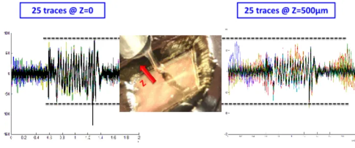
Figure 1 illustrates the principle of these experiments and reports 25 EM measurements obtained at Z = 0 and Z = 500µm while the AES ciphers the same plaintext. The black thick traces are the mean of the 25 measures. One can observe that the amplitudes of the measurements performed at Z = 500µm are lower than the ones at Z = 0, but above all, that some large amplitude noises alter some traces. These spurious noises render the reading of traces less intelligible. Indeed, contrarily to measures at Z = 0, the rounds of the AES are less visible, and completely disappear in the noise at Z = 4000µm.
25 traces @ Z=0 25 traces @ Z=500µm
Fig. 1. 25 EM Measures EM collected at Z = 0 and Z = 500µm above an AES mapped into an FPGA
5.2 Analysis of the experimental results
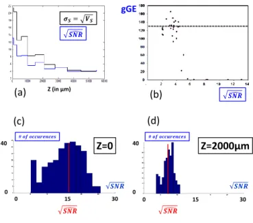
A CPA was applied to each set of 5000 traces collected at Z values ranging between 0 and 5mm. Figure 2 gives the evolution with Z of σS and
p \ SN R. As expected the \SN R decreases rapidly when Z increases; the distributions of the estimated \SN R values (with Equation 2) for Z = 0 and Z = 2000µm are given
Figures 2c and Figures 2d, respectively. For measures done at Z = 0,p\SN R is equal to 15.11 and σ√ SN Ris equal to 4.80 while at Z = 2000µm, p \ SN R is equal to 7.31 and σ√
SN R to 1.64. This demonstrates that the SNR is, as expected, a measure of the quality of the experimental protocol.
Figure 2b gives the evolution of the global Guessing Entropy (gGE) with respect top\SN R. One can observe that the lower thepSN R value is, the less\ efficient the CPA is. In addition, as soon as p\SN R is lower than 5, the CPA does not succeed in disclosing the correct key with 5000 traces and more over the gGE remains close to 128.
Nevertheless, Figure 2b highlights the existence of a link between gGE and the SNR. The standard electrical engineering definition of the SNR (Equation 2) is therefore a figure of merit of the quality of EM traces from an adversary point of view, as the SNR definition considered in [10] and [1]. The higher the \
SN R associated to a set of traces is, the leakier it is expected to be. However, it should be noticed that this figure of merit does not indicate possible problems that can encounter adversaries to exploit this information. These difficulties are for instance:
– the presence or the absence of countermeasures such as masking [3], – the choice of the adequate distinguisher [6], [2],
– the identification of the accurate leakage model [11], which are problems independent from the measurement quality.
6
Collision Criterion for analyzing leakage traces
At that stage, the BCDC has been used for estimating the SNR (Equation 2). Then it has been experimentally shown that this criterion is also a figure of merit to gauge the quality of a set of EM traces with the intent to apply an SCA on it.
The BCDC can also be used to analyze the computational activity of a DUT over time. Indeed, it is quite possible to calculate BCDC values for the different time windows ([ti, · · · , tk] with i ≥ 1 and k ≤ q) constituting the traces:
SN R(ti, · · · , tk) = 1
BCDC2(ti, · · · , tk)− 1 (13) and to deduce \SN R values so that to distinguish windows characterized by different SNR values. This leads to draw the estimated \SN R evolution over time, considering that each type of electrical activity (or instruction) consumes a specific amount of power and is thus characterized by a specific SNR value.
Figure 3 gives 25 EM traces related to the ciphering of 25 random plaintexts (traces with no collision), the standard deviations of all the samples constituting the traces (thus computed with only 25 values), and finally the evolution of p
\
40 Z (in µm) 𝝈𝑺= 𝑽𝑺 𝑺𝑵𝑹 gGE
(a)
(b)
𝑺𝑵𝑹 0 15 30 0 𝑺𝑵𝑹 # 𝒐𝒇 𝒐𝒄𝒄𝒖𝒓𝒆𝒏𝒄𝒆𝒔 # 𝒐𝒇 𝒐𝒄𝒄𝒖𝒓𝒆𝒏𝒄𝒆𝒔 40 0 15 30 0(c)
(d)
Z=0
Z=2000µm
𝑺𝑵𝑹 𝑺𝑵𝑹 𝑺𝑵𝑹Fig. 2. (a) Evolutions with Z of σS and
p \
SN R, (b) Evolution of the gGE wrt the p
\
SN R (c) histogram of the√SN R values estimated with traces collected at Z = 0, (d) histogram of the√SN R values estimated with traces collected at Z = 2000µm
25 traces @ Z=0 𝑺𝑵𝑹(𝒕𝒊 ) 𝝈(𝑻 𝒕𝒊) AES rounds (a) (b) (c)
Fig. 3. (a) 25 EM traces collected @ Z=0 over an AES (b) evolution σ(T (ti)) and (c)
samples, i.e. of duration equal to 0.625 × TCK, with TCK the clock period of the device.
One may observe that even if thep\SN R is high, 25 traces do not allow to clearly localize the AES rounds, nor to interpret the behavior of the device with the vertical standard deviation. More traces are required.
By contrast, 25 traces are largely sufficient, by calculating the \SN R, to locate and identify different phases of activity (loading of the key and the text in the registers, emissions of a trigger signal on an IO, AES computation) of the DUT assuming that each activity phase is characterized by a specific SNR value. In addition, the difference of p\SN R values between active phases and inactive phases is really high.
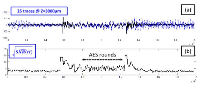
25 traces @ Z=3000µm
𝑺𝑵𝑹(𝒕𝒊 )
AES rounds
(a)
(b)
Fig. 4. (a) 25 EM traces collected @ Z = 3000µm over an AES (b) evolution ofp\SN R
This result may come from two main reasons. The first reason could be the fact that the computation of BCDC values involves the calculus of standard deviations which are performed on a set of 250 consecutive samples rather than 25 values in case of the use of the vertical variance as analysis criterion. This limits the impact of noise. The second could also be related to the reduction of the impact of noise, and more particularly of the effect of outliers. Indeed, 25 traces allows computing the mean of the SNR distribution, \SN R, with 300 different estimates of the SNR.
Figure 4 shows the same results than Figure 3 for 25 traces collected at Z = 3000µm i.e. for traces characterized by a lower SNR value. In this condition the AES is no more visible on the mean trace (in black Figure 4a). In addition, the transitions of a synchronization signal on an IO pad are much more visible; the EM probe is now above the related bonding.
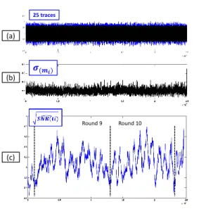
If the results presented above, obtained on an hardware AES embedded on an FPGA, are interesting, the full effectiveness of the technique appears during the analysis of the electrical activity of a micro-controller which executes a software implementation of the AES. To illustrate this, Figure 5 gives 25 traces EM (and their mean) corresponding to the computation of the two last rounds of the AES by a 32-bits processor (cortex M4) designed in 90nm process technology and clocked at 40MHz. As shown, neither the mean nor the variance of traces allow
Round 9 Round 10 25 traces (a) (b) (c) 𝝈(𝒎𝒊)
Fig. 5. (a) 25 EM traces (and their mean in black) collected above a 32bit micro-controller processing an AES (b) evolution σ(mi) and (c) evolution of
p \ SN R
to distinguish any pattern related to the two rounds. The vertical mean and variance look like a really noisy trace. This is not the case with the evolution of \
SN R on which two quite similar (but not exactly the same) patterns are visible. One can even distinguish similar shapes in the two rounds.
7
Collision Criterion for adaptive filtering
In the preceding paragraphs, the BCDC has been exploited to analyze the evo-lution of the electrical activity of two DUT, an FPGA and a micro-controller, using a sliding windowing solution. Such an approach can be adopted to distin-guish in the frequency domain, the frequencies carrying information related to the signal from those that convey essentially noise.
At that end, a frequency bandwidth, δf , is chosen. The colliding traces are then translated in the frequency domain using for example the FFT. This done, for each frequency f of the spectrum, the harmonics falling out of the frequencies bandwidth of interest (f ± δf ) are canceled before to translate back the traces in the time domain and computeSN R(f ± δ) at each frequency f of the spectrum,\ as in the preceding sections.
It should be noticed that δf could be set to the spectral resolution of the FFT which depends on the number of points constituting the traces. This approach with the minimal possible δf value has a larger computational cost and returns in computingSN R(f ) i.e. in keeping only one frequency in the bandwidth.\
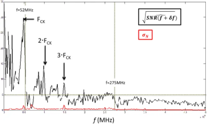
f (MHz) 𝑺𝑵𝑹(𝒇 + 𝜹𝒇) 𝝈𝑵 f=52MHz f=275MHz FCK 2FCK 3FCK
Fig. 6.SN R(f ) and σ\ N(f ) computed with 8 EM traces
Figure 6 gives the evolution with f of SN R(f ± δf ) estimated with only\ 8 EM traces collected above the AES mapped into the FPGA, considering a frequencies bandwidth δf = 2MHz. The quite flat evolution of σN(f ± δf ) is also drawn in this figure.
Contrarily to σN(f ± δf ), SN R(f ± δf ) seems to decrease following a\ f1 function as indicated by the leakage model in the frequency domain introduced in [17] and as formerly observed in [12]. However, it should be noticed that peaks ofSN R(f ± δf ) appear at several multiples of the frequencies (50MHz). This is\ probably due to the influence of the clock tree circuit, one of the largest energy consumers at these frequencies in IC.
More importantly, it should be observed that SN R(f ± δf ) remains high\ (> 5) for f < 275MHz and particularly high for f < 52MHz. It therefore seems wise to only keep harmonics below 275MHz or even 52MHz during SCA.
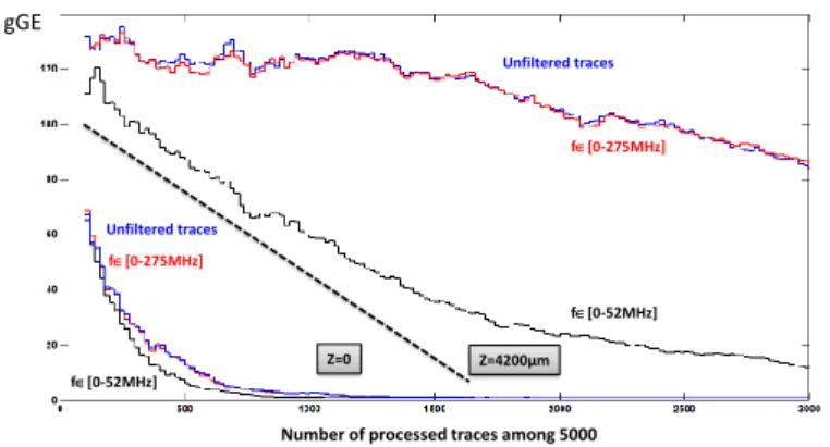
In order to validate thatSN R(f ± δf ) is an interesting figure of merit allow-\ ing to adapt at best the filtering steps usually applied prior any SCA, CPA were first launched on the rough EM traces, then on these same traces after canceling of harmonics higher than 52MHz and 275MHz, respectively. Figure 7 gives the evolutions of the gGE for these three CPA in the case of traces collected at Z = 0 and at Z = 4200µm.
Figure 7 shows that the filtering of traces characterized by a high SNR value (traces collected at Z = 0) has a really limited interest as it was expected. By contrast, for traces collected at Z = 4200µm, characterized by a \SN R value lower than 3, keeping harmonics with the highestSN R(f ± δf ) values allows to\ enhance significantly the efficiency of the CPA. Indeed, keeping only the f values lower than 52MHz allows reaching a gGE lower than 20 after the processing of 3000 traces, value to be compared to 90 without application of any filtering procedure.
Z=4200µm Z=0 Unfiltered traces f[0-275MHz] f[0-52MHz] f[0-275MHz] f[0-52MHz]
Number of processed traces among 5000 gGE
Unfiltered traces
Fig. 7. Evolution of gGE with the number of processed traces (collected either at Z=0 or at Z = 4200µm when keeping respectively all harmonics (in blue), harmonics below 275MHz (in red) and harmonics below 52MHz (in black).
8
Conclusion
The SNR, as defined in engineering, is a key figure for gauging the quality of analogue measurements or communication channels. However, its use requires the knowledge of the signal to be measured. In the context of SCA, the nature and characteristics of the measured signals are not known. The use of the SNR is therefore particularly difficult.
In this context the paper proposes a method to estimate the SNR, when the signal is not known. This method is based on a collision detection criterion. Its advantages are its easiness of use, its accuracy, and its low computation time. It has also been shown in this paper that the SNR is an interesting figure of merit to gauge the quality of SCA traces, to analyze the behavior of IC, or to guide rationally (and therefore in an efficient way) the filtering step commonly used as pre-processing of traces. There are also other applications of this fast SNR estimation method. Among them it use for the spatial analysis IC activity has given interesting results not shown in this paper by lack of place.
However, we believe that the main interest of the proposed SNR estimation technique is that it is a sufficiently simple, low cost and convenient technique to establish the electrical engineering SNR as a standard measure for compar-ing the various experimental practices of SCA of both academic and industrial laboratories.
References
1. S. Bhasin, J.-L. Danger, S. Guilley, and Z. Najm. NICV: normalized inter-class variance for detection of side-channel leakage. IACR Cryptology ePrint Archive, 2013:717, 2013.
2. E. Brier, C. Clavier, and F. Olivier. Correlation power analysis with a leakage model. In Cryptographic Hardware and Embedded Systems - CHES 2004: 6th In-ternational Workshop, 2004, pages 16–29, 2004.
3. S. Chari, C. S. Jutla, J. R. Rao, and P. Rohatgi. Towards sound approaches to counteract power-analysis attacks. pages 398–412. Springer-Verlag, 1999.
4. A. Dehbaoui, V. Lomn´e, P. Maurine, L. Torres, and M. Robert. Enhancing elec-tromagnetic attacks using spectral coherence based cartography. In VLSI-SoC: Technologies for Systems Integration - 17th IFIP WG 10.5/IEEE International Conference on Very Large Scale Integration, VLSI-SoC 2009, 2009, pages 135– 155, 2009.
5. P.-A. Fouque and F. Valette. The doubling attack - Why Upwards Is Better than Downwards. In Cryptographic Hardware and Embedded Systems - CHES 2003, 5th International Workshop, 2003, pages 269–280, 2003.
6. B. Gierlichs, L. Batina, P. Tuyls, and B. Preneel. Mutual information analysis. In Cryptographic Hardware and Embedded Systems - CHES 2008, 10th International Workshop, 2008., pages 426–442, 2008.
7. S. Guilley, H. Maghrebi, Y. Souissi, L. Sauvage, and J-L. Danger. Quantifying the quality of side channel acquisitions. In COSADE, 2011.
8. Diop I., Liardet P-Y, Linge Y., and Maurine P. Collision based attacks in practice. In CRYPTO’PUCES, 2015.
9. P. C. Kocher, J. Jaffe, and B. Jun. Differential power analysis. In Advances in Cryptology - CRYPTO ’99, 19th Annual International Cryptology Conferences, 1999, pages 388–397, 1999.
10. S. Mangard. Hardware countermeasures against dpa ? a statistical analysis of their effectiveness. In CT-RSA, pages 222–235, 2004.
11. Stefan Mangard, Elisabeth Oswald, and Thomas Popp. Power analysis attacks: Revealing the secrets of smart cards, volume 31. Springer Science & Business Media, 2008.
12. E. Mateos and C. H. Gebotys. A new correlation frequency analysis of the side channel. In Proceedings of the 5th Workshop on Embedded Systems Security, WESS 2010, page 4, 2010.
13. D. R´eal, F. Valette, and M. Drissi. Enhancing correlation electromagnetic attack using planar near-field cartography. In Design, Automation and Test in Europe, DATE 2009, pages 628–633, 2009.
14. L. Sauvage, S. Guilley, F. Flament, J.-L. Danger, and Y. Mathieu. Blind cartog-raphy for side channel attacks: Cross-correlation cartogcartog-raphy. Int. J. Reconfig. Comp., 2012:360242:1–360242:9, 2012.
15. K. Schramm, T. Wollinger, and C. Paar. A new class of collision attacks and its application to DES. In Fast Software Encryption, 10th International Workshop, FSE 2003, pages 206–222, 2003.
16. Fran¸cois-Xavier Standaert, Tal Malkin, and Moti Yung. A Unified Framework for the Analysis of Side-Channel Key Recovery Attacks. In EUROCRYPT, pages 443–461, 2009.
17. S. Tiran, S. Ordas, Y. Teglia, M. Agoyan, and P. Maurine. A model of the leakage in the frequency domain and its application to CPA and DPA. J. Cryptographic Engineering, 4(3):197–212, 2014.
18. S.-M. Yen, W.-C. Lien, S.-J. Moon, and J. Ha. Power analysis by exploiting cho-sen message and internal collisions - vulnerability of checking mechanism for rsa-decryption. In Progress in Cryptology - Mycrypt 2005, First International Confer-ence on Cryptology, 2005, pages 183–195, 2005.