HAL Id: hal-00413519
https://hal.archives-ouvertes.fr/hal-00413519
Submitted on 4 Sep 2009
HAL is a multi-disciplinary open access
archive for the deposit and dissemination of
sci-entific research documents, whether they are
pub-lished or not. The documents may come from
teaching and research institutions in France or
L’archive ouverte pluridisciplinaire HAL, est
destinée au dépôt et à la diffusion de documents
scientifiques de niveau recherche, publiés ou non,
émanant des établissements d’enseignement et de
recherche français ou étrangers, des laboratoires
Domain decomposition algorithms for the compressible
Euler equations
Victorita Dolean, Frédéric Nataf
To cite this version:
Victorita Dolean, Frédéric Nataf. Domain decomposition algorithms for the compressible Euler
equa-tions. G. Galdi, J.G. Heywood, R. Rannacher Edts. Analysis and Simulation for Fluid Dynamics,
Birkhauser, pp.69-88, 2007, Advances in Mathematical Fluid Mechanics. �hal-00413519�
Domain decomposition algorithms for the compressible Euler
equations
V. Dolean
∗, F. Nataf
†15th September 2005
Abstract
In this work we present an overview of some classical and new domain decomposition methods for the resolution of the Euler equations. The classical Schwarz methods are formulated and analyzed in the framework of first order hyperbolic systems and the differences with respect to the scalar problems are presented. This kind of algorithms behave quite well for bigger Mach numbers but we can further improve their performances in the case of lower Mach numbers. There are two possible ways to achieve this goal. The first one implies the use of the optimized interface conditions depending on a few parameters that generalize the classical ones. The second is inspired from the Robin-Robin preconditioner for the convection-diffusion equation by using the equivalence via the Smith factorization with a third order scalar equation.
1
Introduction
When solving the compressible Euler equations by an implicit scheme the nonlinear system is usually solved by Newton’s method. At each step of this method we have to solve a linear system which is non-symmetric and very ill conditioned. The necessity of a domain decomposition became more and more obvious. In a previous paper [DLN04] we formulated a Schwarz algorithm (interface iteration which relies on the successive solving of the local decomposed problems and the transmission of the result at the interface) involving transmission conditions that are derived naturally from a weak formulation of the underlying boundary value problem (first formulated in [QS96]). As far as these algorithms are con-cerned, when dealing with supersonic flows, whatever the space dimension is, imposing the appropriate characteristic variables as interface conditions leads to a convergence of the algorithm which is optimal with regards to the number of subdomains. The only case of interest remains the subsonic one where this property is lost except in the one dimensional case. We recall briefly these results in order to introduce more general and performant methods such as the optimized interface conditions and the preconditioning methods. The former were widely studied and analyzed for scalar problems such as elliptic equations in [Lio90, EZ98], for the Helmholtz equation in [BD97, CN98] convection-diffusion problems in [JNR01]. For time dependent problems and local times steps, see for instance [GHN01]. The preconditioning methods have also known a wide developpement in the last decade. The Neumann-Neumann algorithms for sym-metric second order problems [RT91] has been the subject of numerous works, see [TW04] and references therein. An extension of these algorithms to non-symmetric scalar problems (the so called Robin-Robin algorithms) has been done in [ATNV00, GGTN04] for advection-diffusion problems.
In the section 2 we first formulate the Schwarz algorithm for a general linear hyperbolic system of PDEs with general interface conditions inspired by Clerc [DN04b] built in order to have a well-posed problem. The convergence rate is computed in the Fourier space as a function of some parameters. We will further
∗Univ. de Nice and INRIA, Sophia Antipolis, 06108 Nice Cedex 02, France, [email protected]
estimate the convergence rate at the discrete level. We will find the optimal parameters of the interface conditions at the discrete level. We will then use the new optimal interface conditions in Euler compu-tations which illustrate the improvement over the classical interface conditions (first described in [QS96]). As far as preconditioning methods are concerned, to our knowledge, no extension to the Euler equa-tions was done. In the section 2 we will first show the equivalence between the 2D Euler equaequa-tions and a third order scalar problem, which is quite natural by considering a Smith factorization of this system, see [Gan66] then we define an optimal algorithm for the third order scalar equation inspired from the idea of the Robin-Robin algorithm [ATNV00] applied to a convection-diffusion problem. Afterwards we back-transform it and define the corresponding algorithm applied to the Euler system. All the previous results have been obtained at the continuous level and for a decomposition into 2 unbounded subdomains. After a discretization in a bounded domain we cannot expect that these properties to be preserved exactly. Still we can show by a discrete convergence analysis that the expected results should be very good.
2
A Schwarz algorithm with general interface conditions
In this section introduce a Schwarz algorithm which is based on general transmission conditions at subdomain interfaces that take into account the hyperbolic nature of the problem. In addition, we recall some existing results concerning the convergence of the algorithm. We consider here a general non-linear system of conservation laws. Under the hypothesis that the solution is regular, we can also write it under a non-conservative (or quasi-linear) equivalent form:
(1) ∂W ∂t + d ! i=1 Ai(W )∂W ∂xi = 0
where the Aiare the Jacobian matrices of the flux vectors. Assume that we first proceed to an integration
in time of (1) using a backward Euler implicit scheme involving a linearization of the flux functions and eventually we symmetrize it (we know that when the system admits an entropy it can be symmetrized by multiplying it by the hessian matrix of this entropy). This operation results in the linearized system:
(2) L(δW ) ≡ Id ∆tδW + d ! i=1 Ai∂δW ∂xi = f
In the following we will define the boundary conditions that have to be imposed when solving the problem on a domain Ω ⊂ Rd. We denote by A
n = "di=1Aini, the linear combination of jacobian matrices by
the components of the outward normal vector at the boundary of the domain ∂Ω. This matrix is real, symmetric and can be diagonalized
An= T ΛnT−1, Λn= diag(λi)
It can also be splitted in negative and positive part using this diagonalization
An= A+n+ A−n, A±n= T Λn±T−1, Λ+n = diag(max(λi, 0)), Λ−n = diag(min(λi, 0))
This corresponds to a decomposition with local characteristic variables. A more general splitting in negative(positive) definite parts, Aneg
n and Aposn of An can be done such that these matrices satisfy the
following properties:
(3) An= Anegn + Aposn , rank(Aneg,posn ) = rank(A±n), A pos
−n= −Anegn
In the scalar case the only possible choice is Aneg
n = A−n. Using the previous formalism we can define the
following boundary condition:
Remark 1 In the case of a classical decomposition in negative and positive part this boundary condition has the physical meaning of the incoming flux in domain Ω. By extension of the properties found in this case we call the last equality of (3) conservation property because it insures that the “out-flow” quantity (given by the positive part of the jacobian flux matrix with oposite direction of the normal) is retrieved out of the “in-flow” quantity imposed by the boundary condition (given the negative part of the jacobian flux matrix).
2.1
Schwarz algorithm with general interface conditions
We consider a decomposition of the domain Ω into N overlapping or non-overlapping subdomains ¯Ω = #N
i=1¯Ωi. We denote by nij the outward normal to the interface Γij bewteen Ωi and a neighboring
subdomain Ωj. Let Wi(0) denote the initial appoximation of the solution in subdomain Ωi. A general
formulation of a Schwarz algorithm for computing (Wp+1
i )1≤i≤N from (Wip)1≤i≤N (where p defines the
iteration of the Schwarz algorithm) reads :
(4) LWip+1 = f in Ωi AnegnijW p+1 i = AnegnijW p j on Γij = ∂Ωi∩ Ωj Aneg nijW p+1 i = Anegnijg on ∂Ω ∩ ∂Ωi where Aneg nij and A pos
nij satisfy (3). We have the following result concerning the convergence of the Schwarz
algorithm in the non-overlapping case, due to([Cle98]): Theorem 1 If we denote by Ep
i = W
p
i − Wi the error vector associated to the restriction to the i-th
subdomain of the global solution of the problem. Then, the Schwarz algorithm converges in the following
sense : lim p→∞%E p i%L2(Ωi)q = 0 lim p→∞% d ! j=1 Aj∂jEpi%L2(Ωi)q = 0
The convergence rate of the algorithm defined by (4) depends of the choice of the decomposition of Anij
into a negative and a positive part satisfying (3). In order to choose the decomposition (3) we need to relate this choice to the convergence rate of (4).
2.2
Convergence rate of the algorithm with general interface conditions
We consider a two-subdomain non-overlapping or overlapping decomposition of the domain Ω = Rd,
Ω1 =] − ∞, γ[×Rd−1 and Ω2 =]β, ∞[×Rd−1 with β ≤ γ and study the convergence of the Schwarz
algorithm in the subsonic case. A Fourier analysis applied to the linearized equations allows us to derive the convergence rate of the “ξ”-th Fourier component of the error. We will first briefly recall the technique of Fourier transform which was already described in detail in [DLN04]. The vector of Fourier variables is denoted by ξ = (ξj, j = 2, . . . , d). Let (Eip)(x) = (W
p
i − Wi)(x) be the error vector in the ith subdomain
at the pth iteration of the Schwarz algorithm and: ˆ
E(x1, ξ2, . . . , ξd) = FE(x1, ξ2, . . . , ξd) =
(
Rd−1
e−iξ2x2−...−iξdxdE(x
1, . . . , xd)dx2. . . dxd
the Fourier symbol of the error vector. This transformation is useful only if the Ai matrices are constant
which is the case here because we have considered the linearized form of the Euler equations around a constant state ¯W . The Schwarz algorithm in the Fourier space (ξ∈ Rd−1) can be written as follows:
(5) d dx1 ˆ E1p+1 = −M(ξ) ˆE1p+1, x < γ Aneg( ˆEp+1 1 ) = Aneg( ˆE p 2), on x = γ d dx1 ˆ E2p+1 = −M(ξ) ˆE2p+1, x > β Apos( ˆEp+1 2 ) = Apos( ˆE p 1), on x = β
where we denoted by Aneg = Aneg
n , Apos = Aposn with n = (1, 0) the outward normal to the domain Ω1
and: (6) M (ξ) = A−11 ) 1 ∆tId + d ! i=2 Aiξi−1 *
We thus obtain local problems that for a given ξ are very simple ODEs whose solutions can be expressed as linear combinations of the eigenvectors of M(ξ) (we denote by λj(ξ) the eigenvalues of M(ξ)). Here
we require that these solutions are bounded at infinity (−∞ and +∞ respectively). We deduce that in the decomposition of ˆE1(x1, ξ) (respectively ˆE2(x1, ξ)) we must keep only the eigenvectors
correspond-ing to the negative (respectively the positive) real parts of the eigenvalues. Takcorrespond-ing into account these considerations we replace the expressions of the local solutions into the interface conditions (5) to obtain the interface iterations on the α coefficients:
(α1,p+1 j )j,%(λj)<0(ξ) = T1 + (α2,p j )j,%(λj)>0(ξ) , (α2,p+1 j )j,%(λj)>0(ξ) = T2 + (α1,p j )j,%(λj)<0(ξ) ,
Then, the convergence rate of the ξ-th component of the error vector of the Schwarz algorithm can be computed as the spectral radius of one of the iteration matrices T1T2(ξ) or T2T1(ξ):
ρ2
2≡ ρ2Schwarz2= ρ(T1T2) = ρ(T2T1)
2.3
The 2D Euler equations
After having defined in a general frame the well-possedness of the boundary value problem associated to a general equation and the convergence of the Schwarz algorithm applied to this class of problems, we will concentrate ourselves on the conservative Euler equations in two-dimensions:
(7) ∂W ∂t + ∇.F (W ) = 0 , W = (ρ, ρV , E) T , ∇ = - ∂ ∂x, ∂ ∂y .T .
In the above expressions, ρ is the density, V = (u, v)T is the velocity vector, E is the total energy
per unit of volume and p is the pressure. In equation (7), W = W (x, t) is the vector of conservative variables, x and t respectively denote the space and time variables and F (W ) = (F1(W ) , F2(W ))T is
the conservative flux vector whose components are given by
F1(W ) = ρu ρu2+ p ρuv u(E + p) , F2(W ) = ρv ρuv ρv2+ p v(E + p) .
The pressure is deduced from the other variables using the state equation for a perfect gas p = (γs− 1)(E −12ρ% V %2) where γs is the ratio of the specific heats (γs= 1.4 for the air).
2.4
A new type of interface conditions
We will apply now the method described previously to the computation of the convergence rate of the Schwarz algorithm applied to the two-dimensional subsonic Euler equations. In the supersonic case there is only one decomposition satisfying (3), that is: Apos= A
nand Aneg= 0 and the convergence follows
in 2 steps. Therefore the only case of interest is the subsonic one. The starting point of our analysis is given by the linearized form of the Euler equations (7) which are of the form (2) where we replace δW
by W and to whom we applied a change of variable ˜W = T−1W based on the eigenvector factorization
of A1= T ˜A1T−1. In the following we will abandon the ˜ symbol):
W
c∆t+ A1∂xW + A2∂yW = 0
characterized by the jacobian matrices A1 and A2 depending on Mn = uc, Mt = vc which denote
re-spectively the normal and the tangential Mach number. Before estimating the convergence rate we will derive the general transmission conditions at the interface by splitting the matrix A1 into a positive and
negative part.
We have the following general result concerning this decomposition:
Lemma 1 Let λ1 = Mn− 1, λ2 = Mn+ 1, λ3 = λ4 = Mn. Suppose we deal with a subsonic flow:
0 < u < c so that λ1 < 0, λ2,3,4 > 0. Any decomposition of A1= An, n = (1, 0) which satisfies (3) has
to be of the form: Aneg= 1 a1u · u t, u = (a 1, a2, a3, a4)t Apos= A n− Aneg.
where (a1, a2, a3, a4) ∈ R4 satisfies a1≤ λ1< 0 and aλ11 + a
2 2 a1λ2 + a23 a1λ3 + a24 a1λ4 = 1.
For the details of the proof see [DN04b].
We will proceed now to the estimation of the convergence rate using some results from [DLN04]. Following the technique described in section 2.2 we estimate the convergence rate in the non-overlapping case and we use the non-dimensioned wave-number ¯ξ = c∆tξ and if we drop the bar symbol, we get for the general interface conditions the following:
(8) ρ2 2,novr(ξ) = 5 5 51 − 4Mn(1−Mn)(1+Mn)R(ξ)a21(a+MnR(ξ)) D1D2 5 5 5 D1 = R(ξ)[a1(1 + Mn) − a2(1 − Mn)] + a[a1(1 + Mn) + a2(1 − Mn)] − i√2a3ξ(1− Mn2) D2 = Mna1[R(ξ)[a1(1 + Mn) − a2(1 − Mn)] + a[a1(1 + Mn) + a2(1 − Mn)]] + a3(1 − Mn2)[a3(R + a) − iMna1ξ√2]
Remark 2 The expression (8) gives the convergence rate in the classical case for a1= −(1−Mn) = λ1(0)
and a2 = a3= a4 = 0, which corresponds to the classical transmission conditions. Moreover, theorem 1
proves that this quantity is always strictly inferior to 1 as the algorithm is convergent.
In order to simplify our optimization problem we will take a3 = 0, we can thus reduce the number of
parameters to 2, a1and a2, as we can see that a4can be expressed as a function of a1, a2and a3. We can
also see that the convergence rate is a real quantity when the flow is normal to the interface Mt= 0. In
the same time for the optimization purpose only we introduce the parameters: b1 = −a1/(1− Mn) and
b2= a2/(1 + Mn) which provide a simpler form of the convergence rate:
(9) ρ22,novr(ξ) = 5 5 5 51 −(R(ξ)(b14b+ b1(a + M2) + a(bnR(ξ))R(ξ)1− b2))2(Mn + 1) 5 5 5 5
Before proceeding to the analysis of the general case we recall some results found in the classical case obtained in [DLN04]. The asymptotic convergence rate in the non-overlapping case:
(10) lim k→+∞ρ2,novr(k) = 6-1 − 3Mn 1 + Mn .2 + 8MnMt2 (1 + Mn)3 < 1
is always strictly inferior to 1. Moreover, in the particular case M#
n = 1/3 and Mt= 0, this limit becomes
null. The inequality (10) has a numerical meaning. For a given discretization, let ξmaxdenote the largest
frequency supported by the numerical grid. This largest frequency is of the order π/h with h a typical mesh size. The convergence rate in a numerical computation made on this grid can be estimated by ρh
2 = max|ξ|<ξmaxρ2(ξ). From (10), we have that ρh2 ≤ max|ξ|<ξmaxρ2(ξ) < 1. This means that for finer
and finer grids, the number of iterations may increase slightly but should not go to infinity. Thus the optimization problem with respect to the parameters b1 and b2, makes sense:
(11) min
(b1,b2)∈I1×I2(b1)maxξ≥0 ρ(ξ)
The solving of this problem is quite a tedious task even in the non-overlapping case, where we can obtain analytical expression of the parameters only for some values of the Mach number. In the same time, we have to analyze the convergence of the overlapping algorithm. Indeed, standard discretizations of the interface conditions correspond to overlapping decompositions with an overlap of size δ = h, h being the mesh size, as seen in [CFS98] and [DLN04]. Analytic optimization with respect to b1 and b2 seems out
of reach. We will have to use numerical procedures of optimization.
In order to get closer to the numerical simulations we will estimate the convergence rate for the dis-cretized equations with general transmission conditions, both in the non-overlapping and the overlapping case and then optimize numerically this quantity in order to get the best parameters for the conver-gence. Following a similar procedure as that described in [DLN04] and [DN04b] we will first discretize the problem by a finite volume scheme then we formulate a Schwarz algorithm whose convergence rate is estimated at the discrete level. Therefore, we will get the theoretical optimized parameters at the discrete level by means of a numerical algorithm, by calculating the following
(12) ρ(b1, b2) = maxk∈Dhρ
2
2(k, ∆x, Mn, Mt, b1, b2)
min(b1,b2)∈Ihρ(b1, b2)
where Dhis a uniform partition of the interval [0, π/∆x] and Ih ⊂ I a discretization by means of a uniform
grid of a subset of the domain of the admissible values of the parameters. This kind of calculations are done once for all for a given pair (Mn, Mt) before the beginning of the Schwarz iterations. An example of
such a result is given in the figure 1 Mach number Mn= 0.2. The computed parameters from the relation
(12) will be further refered to with a superscript th. The theoretical estimates are compared afterwards with the numerical ones obtained by running the Schwarz algorithm with different pairs of parameters which lie in a an interval such that the algorithm is convergent. We are thus able to estimate the optimal values for b1and b2from these numerical computations. These values will be referred to by a superscript
num.
2.5
Implementation and numerical results
We present here a set of results of numerical experiments that are concerned with the evaluation of the influence of the interface conditions on the convergence of the non-overlapping Schwarz algorithm of the form. The computational domain is given by the rectangle [0 , 1] × [0 , 1]. The numerical investigation is limited to the resolution of the linear system resulting from the first implicit time step using a Courant number CFL=100. In all these calculations we considered a model problem: a flow normal to the inter-face (that is when Mt = 0). In figures 1 and 2 we can see an example of a theoretical and numerical
estimation of the reduction factor of the error. We illustrate here the level curves which represent the log of the precision after 20 iterations for different values of the parameters (b1, b2), the minimum being
attained in this case for bth
1 = 1.3 and bth2 = −0.5, bnum1 = 1.4 and bnum2 = −0.6. We can see that we have
good theoretical estimates of these parameters we can therefore use them in the interface conditions of the Schwarz algorithm.
Table 1: Overlapping Schwarz algorithm Numerical vs. theoretical parameters
Mn bth1 bth2 bnum1 bnum2 0.1 1.6 -0.8 1.6 -0.9 0.2 1.3 -0.5 1.4 -0.6 0.3 1.25 -0.3 1.25 -0.45 0.4 1.08 -0.15 1.08 -0.28 0.5 1.03 -0.08 1.02 -0.23 0.6 1.0 0.0 1.0 0.0 0.7 1.02 0.06 1.01 0.04 0.8 1.03 0.08 1.02 0.06 0.9 1.06 0.08 1.04 0.06 −1 −0.9 −0.8 −0.7 −0.6 −0.5 −0.4 −0.3 −0.2 −0.1 0 1 1.1 1.2 1.3 1.4 1.5 1.6 1.7 1.8 1.9 2 b2 b1
Theoretical optimization: Mn=0.2, predicted precision after 20 iterations
−5.2 − 5.2 − 5.2 −5 − 5 − 5 −5 − 5 −4.8 −4.8 −4.8 − 4.8 −4.8 − 4.8 − 4.6 −4.6 −4.6 −4.6 − 4.6 −4.6 −4.4 −4.4 −4.4 − 4.4 − 4.4 −4.4 −4.2 −4.2 −4.2 − 4.2 − 4.2 −4.2 −4 −4 −4 −4 − 4 − 4 −4 −3.8 −3.8 −3.8 − 3.8 −3.8 − 3.8 −3.6 −3.6 −3.6 −3.6 − 3.6 −3.6 −3.4 −3.4 −3.4 − 3.4 − 3.4 −3.4 −3.2 −3.2 − 3.2 − 3.2 − 3.2 −3 −3 −3 − 3 − 3 − 3 −2.8 −2.8 − 2.8 − 2.8 − 2.8 −2.6 −2.6 −2.4 −2.4 −2.2 −2.2 −2 −2 −1.8 −1.8 −1.6 −1.6 −1.4 −1.4 −1.2 −1.2 −1 −1 −0.8 −0.8 −0.6 −0.6 −0.4 −0.4 −0.2 −0.2 0 0 −5 −4.5 −4 −3.5 −3 −2.5 −2 −1.5 −1 −0.5 0
Figure 1: Isovalues of the predicted reduction factor of the error after 20 iterations via formula (12)
−1 −0.9 −0.8 −0.7 −0.6 −0.5 −0.4 −0.3 −0.2 −0.1 0 1 1.1 1.2 1.3 1.4 1.5 1.6 1.7 1.8 1.9 2 b2 b1
Numerical optimization:Mn=0.2, precision attained in 20 iterations
− 6 −6 −6 −6 −5.6 −5.6 −5.6 −5.6 −5.6 −5.2 −5.2 −5.2 −5.2 −5.2 −4.8 −4.8 −4.8 −4.8 −4.8 −4.8 −4.4 −4.4 −4.4 −4.4 −4.4 −4.4 −4 −4 −4 − 4 −4 −4 −4 −3.6 −3.6 −3.6 −3.6 −3.6 −3.6 −3.6 −3.2 −3.2 −3.2 −3.2 −3.2 −3.2 −2.8 −2.8 − 2.8 −2.8 −2.8 −2.4 −2.4 −2.4 −2 −2 −1.6 −1.6 −1.2 −1.2 −0.8 −0.8 −0.4 −0.4 0 0 −6 −5 −4 −3 −2 −1 0
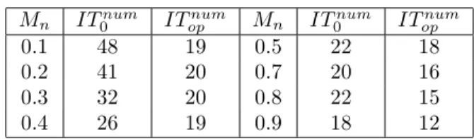
Table 2: Overlapping Schwarz algorithm Classical vs. optimized counts for different values of Mn
Mn IT0num ITopnum Mn IT0num ITopnum
0.1 48 19 0.5 22 18 0.2 41 20 0.7 20 16 0.3 32 20 0.8 22 15 0.4 26 19 0.9 18 12
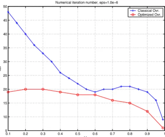
Table 2 summarizes the number of Schwarz iterations required to reduce the initial linear residual by a factor 10−6 for different values of the reference Mach number with the optimal parameters bnum
1 and
bnum
1 . Here we denoted by IT0numand ITopnumthe observed (numerical) iteration number for classical and
optimized interface conditions in order to achieve a convergence with a threshlod ε = 10−6. The same
results are presented in figure 4. In the figure 3 we compare the theoretical estimated iteration number in the classical and optimized case. Comparing figures 3 and 4 we can see that the theoretical prediction are very close to the numerical tests.
0.1 0.2 0.3 0.4 0.5 0.6 0.7 0.8 0.9 1 0 10 20 30 40 50 60 Mn Iter
Theoretical iteration number, eps=1.0e−6
Classical Ovr. Optimized Ovr.
Figure 3: Theoretical iteration number: classical vs. optimized conditions
The conclusion of these numerical tests is, on one hand, that the theoretical prediction is very close to the numerical results: we can get by a numerical optimization (12) a very good estimate of optimal parameters (b1, b2)). On the other hand, the gain, in number of iterations, provided by the optimized
interface conditions, is very promising for low Mach numbers, where the classical algorithm doesn’t give optimal results. We can note that the optimized convergence rate is monotone with respect to the normal Mach number while the classical one isn’t. For bigger Mach numbers, for instance, those who are close to 1, the classical algorithm already has a very good behaviour so the optimization is less useful. In the same time we studied here the zero order and therefore very simple transmission conditions. The use of higher order conditions (see [GMN02]) is a possible way that can be further studied to obtain even better convergence results.
3
A new preconditioning method
In this section we will show the equivalence between the linearized Euler system and a third order scalar equation. The motivation for this transformation is that a new algorithm is easier to design for a scalar
0.1 0.2 0.3 0.4 0.5 0.6 0.7 0.8 0.9 1 5 10 15 20 25 30 35 40 45 50 Mn Iter
Numerical iteration number, eps=1.0e−6
Classical Ovr. Optimized Ovr.
Figure 4: Numerical iteration number: classical vs. optimized conditions equation than for a system of partial differential equations.
3.1
Equivalence of the Euler system to a scalar equation
The starting point of our analysis is given by the linearized form of the Euler equations (7) written in primitive variables (p, u, v, S). In the following we suppose that the flow is isentropic, which allows us to drop the equation of the entropy (which is totally decoupled with respect to the others). We denote by W = (P, U, V )T the vector of unknowns and by A and B the jacobian matrices of the fluxes F
i(w) to
whom we already applied the variable change from conservative to primitive variables. In the following, we shall denote by ¯c the speed of the sound and we consider the linearized form (we will mark by the bar symbol, the constant state around which we linearize) of the Euler equations:
(13) PW ≡ W
∆t+ A∂xW + B∂yW = f
characterized by the following jacobian matrices:
(14) A = ¯u ¯ρ¯c2 0 1/¯ρ ¯u 0 0 0 ¯u B = ¯v 0 ¯ρ¯c2 0 ¯v 0 1/¯ρ 0 ¯v We can re-write the system (13) by denoting β = 1
∆t > 0 under the form
(15) PW ≡ (βI + A∂x+ B∂y) W = f
We will study this system with the help of the Smith factorization. 3.1.1 Smith factorization
We first recall the definition of the Smith factorization of a matrix with polynomial entries and apply it to systems of PDEs, see [Gan66] and references therein.
Theorem 2 Let n be an integer and C an invertible n × n matrix with polynomial entries in the variable λ : C = (cij(λ))1≤i,j≤n.
• det(E)=det(F )=1 • D is a diagonal matrix. • C = EDF .
Moreover, D is uniquely defined up to a reordering and multiplication of each entry by a constant by a formula defined as follows. Let 1 ≤ k ≤ n,
• Sk is the set of all the submatrices of order k × k extracted from C.
• Detk= {Det(Bk)\Bk ∈ Sk}
• LDk is the largest common divisor of the set of polynomials Detk.
Then,
(16) Dkk(λ) =
LDk(λ)
LDk−1(λ), 1≤ k ≤ n
(by convention, LD0= 1).
Application to the Euler system We first take formally the Fourier transform of the system (15) with respect to y (the dual variable is ξ). We keep the partial derivatives in x since in the sequel we shall consider a domain decomposition with an interface whose normal is in the x direction. We note
(17) P =ˆ β + ¯u∂x+ iξ¯v ¯ρ¯c2∂x i ¯ρ¯c2ξ 1 ¯ ρ∂x β + ¯u∂x+ iξ¯v 0 iξ ¯ ρ 0 β + ¯u∂x+ i¯vξ
We can perform a Smith factorization of ˆP by considering it as a matrix with polynomials in ∂x
entries. We have (18) P = EDFˆ where (19) D = 1 0 0 0 1 0 0 0 L ˆˆG and E = 1 (¯u(¯c2− ¯u2))1/3 i ¯ρ¯c2ξ 0 0 0 ¯u 0 β + ¯u∂x+ i¯vξ E2 ¯c2 − ¯u2 iξ ¯ρ¯c2 and (20) F =− β + ¯u∂x+ iξ¯v iξ ¯ρ¯c2 ∂x iξ 1 ∂x ¯ρ¯u β + ¯u∂x+ iξ¯v ¯u 0 ¯u β + iξ¯v ¯ρ¯u2 β + iξ¯v 0 where E2= ¯u(−¯u¯c 2+ ¯u3)∂
xx+ (2¯u2− ¯c2)(β + iξ¯v)∂x+ ¯u((β + iξ¯v)2+ ξ2¯c2)
(21) G = β + ¯u∂ˆ x+ iξ¯v
and
(22) L = βˆ 2+ 2iξ¯u¯v∂
x+ 2β(¯u∂x+ iξ¯v) + (¯c2− ¯v2)ξ2− (¯c2− ¯u2)∂xx
Equation (19) suggests that the derivation of a domain decomposition method (DDM) for the third order operator LG is a key ingredient for a DDM for the compressible Euler equations.
3.2
A new algorithm applied to a scalar third order problem
In this section we will describe a new algorithm applied to the third order operator found in section 3.1.1. We want to solve
(23) LG(Q) = g
where Q is scalar unknown function and g is a given right hand side. The algorithm will be based on the Robin-Robin algorithm [ATNV00] for the convection-diffusion problem. Then we will prove its convergence in 2 iterations. We first note that the elliptic operator L can also be written as:
(24) L = −div(A∇) + a∇ + β2, A = - ¯c2 − ¯u2 −¯u¯v −¯u¯v ¯c2 − ¯v2 . where a = 2β(¯u, ¯v)
Without loss of generality we assume in the sequel that the flow is subsonic and that ¯u > 0 and thus we have 0 < ¯u < ¯c.
3.2.1 The algorithm for a two-domain decomposition
We consider now a decomposition of the plane R2into two non-overlapping sub-domains Ω
1= (−∞, 0)×R
and Ω2= (0, ∞, 0) × R. The interface is Γ = {x = 0}. The outward normal to domain Ωiis denoted ni,
i = 1, 2. Let Qi,k, i = 1, 2 represent the approximation to the solution in subdomain i at the iteration k
of the algorithm. We define the following algorithm:
ALGORITHM 1 We choose the initial values Q1,0 and Q2,0 such that GQ1,0= GQ2,0 and we compute
(Qi,k+1)
i=1,2 from (Qi,k)i=1,2 by the following iterative procedure:
Correction step We compute the corrections ˜Q1,k and ˜Q2,k as solution of the homogeneous local
prob-lems: (25) LG ˜Q1,k= 0 in Ω1, (A∇ −1 2a)G ˜Q 1,k · n1= γk, on Γ. LG ˜Q2,k= 0 in Ω 2, (A∇ − 1 2a)G ˜Q 2,k · n2= γk, on Γ, ˜ Q2,k= 0, on Γ. where γk= −1 2 7 A∇GQ1,k · n1+ A∇GQ2,k· n28.
Update step.We update Q1,k+1 and Q2,k+1 by solving the local problems:
(26) 9 LGQ1,k+1= g, in Ω 1, GQ1,k+1= GQ1,k+ δk, on Γ. LG ˜Q2,k+1= g, in Ω 2, GQ2,k+1= GQ2,k+ δk, on Γ, Q2,k+1= Q1,k+ ˜Q1,k, on Γ. where δk = 1 2 + G ˜Q1,k+ G ˜Q2,k,.
Proposition 1 Algorithm 1 converges in 2 iterations. For the details of the proof see [DN04a].
3.3
A new algorithm applied to the Euler system
After having found an optimal algorithm which converges in two steps for the third order model problem, we focus on the Euler system by translating this algorithm into an algorithm for the Euler system. It suffices to replace the operator LG by the Euler system and Q by the last component F (W )3 of F (W )
in the boundary conditions. This algorithm is quite complex since it involves second order derivatives of the unknowns in the boundary conditions on GF (W )3. It is possible to simplify it. By using the Euler
equations in the subdomain, we have lowered the degree of the derivatives in the boundary conditions. After lengthy computations that we omit here, we find a simpler algorithm. We write it for a decomposi-tion in two subdomains with an outflow velocity at the interface of domain Ω1 but with an interface not
necessarily rectilinear. In this way, it is possible to figure out how to use for a general domain decom-position. In the sequel, n = (nx, ny) denotes the outward normal to domain Ω1, ∂n = ∇ · n the normal
derivative at the interface, ∂τ= ∇ · τ the tangential derivative, Un = Unx+ V ny and Uτ = −Uny+ V nx
are respectively the normal and tangential velocity at the interface between the subdomains. Similarly, we denote ¯un (resp. ¯uτ) the normal (resp. tangential) component of the velocity around which we have
linearized the equations.
ALGORITHM 2 We choose the initial values Wi,0= (Pi,0, Ui,0, Vi,0), i = 1, 2 such that P1,0= P2,0
and we compute Wi,k+1 from Wi,k by the iterative procedure with two steps:
Correction step We compute the corrections ˜W1,k and ˜W2,k as solution of the homogeneous local
problems: (27) P ˜W1,k= 0, in Ω 1, −(β + ¯uτ∂τ) ˜Un1,n+ ¯un∂τU˜τ1,k= γk, on Γ. P ˜W2,k= 0, in Ω 2, (β + ¯uτ∂τ) ˜Un2,k− ¯un∂τU˜τ2,k= γk, on Γ ˜ P2,k+ ¯ρ¯u nU˜n2,k= 0, on Γ. where γk= −1 2 +
(β + ¯uτ∂τ)(Un2,k− Un1,k) + ¯un∂τ( ˜Uτ1,k− ˜Uτ2,k)
, .
Update step.We compute the update of the solution W1,k+1and W2,k+1as solution of the local problems:
(28) 9 PW1,k+1= f 1, in Ω1, P1,k+1= P1,k+ δk, on Γ. PW2,k+1= f 2, in Ω2, P2,k+1 = P2,k+ δk, on Γ, (P + ¯ρ¯unUn)2,k+1= (P + ¯ρ¯unUn)1,k+ ( ˜P + ¯ρ¯unU˜n)1,k, on Γ. where δk = 1 2 + ˜ P1,k+ ˜P2,k,.
Proposition 2 For a domain Ω = R2divided into two non overlapping half planes, algorithm 2 converges
in two iterations.
For the details of the proof see [DN04a].
3.4
Numerical results
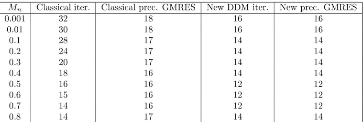
We compare the proposed method and the classical method defined in [DLN04] involving interface condi-tions that are derived naturally from a weak formulation of the underlying boundary value problem. We present here a set of results of numerical experiments on a model problem. We consider a decomposition into different number of subdomains and for a linearization around a constant or non-constant flow. The computational domain is given by the rectangle [0 , 4]×[0 , 1] with a uniform discretization using 80×20 points. The numerical investigation is limited to the solving of the linear system resulting from the first implicit time step using a Courant number CFL=100. For all tests, the stopping criterion was a reduc-tion of the maximum norm of the error by a factor 10−6. In the following, for the new algorithm, each
Mn Classical iter. Classical prec. GMRES New DDM iter. New prec. GMRES 0.001 32 18 16 16 0.01 30 18 16 16 0.1 28 17 14 14 0.2 24 17 14 14 0.3 20 17 14 14 0.4 18 16 14 14 0.5 16 16 12 12 0.6 15 16 12 12 0.7 14 16 12 12 0.8 14 17 14 14
Table 3: Subdomain solves counts for different values of Mn, Mt(y)
h (Mn= 0.001) Classical New DDM h (Mn= 0.1) Classical New DDM
1/10 65 18 1/10 56 12
1/20 67 18 1/20 57 14
1/40 70 18 1/40 59 16
Table 4: Subdomain solves counts for different mesh size
iteration counts for 2 as we need to solve twice as much local problems than with the classical algorithm. For an easier comparison of the algorithms, the figures shown in the tables are the number of subdomains solves.
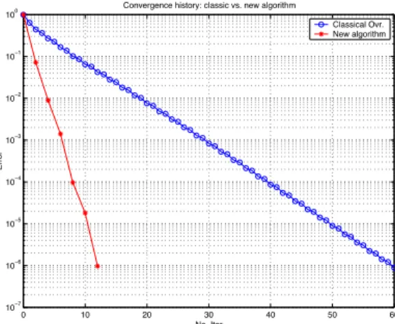
In Table 3, we consider a linearization around a variable state where the tangential velocity is given by Mt(y) = 0.1(1+cos(πy)) and we vary the normal Mach number. In figure 5, we linearize the equations
around a variable state for a normal flow to the interface (Mt= 0.0), where the initial normal velocity is
gives by Mn(y) = 0.5(0.2 + 0.04 tanh(y/0.2))). The sensitivity to the mesh size is shown in the Table 4.
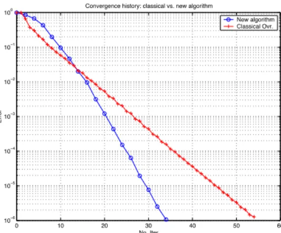
0 10 20 30 40 50 60 10−7 10−6 10−5 10−4 10−3 10−2 10−1 100 No. Iter Error
Convergence history: classic vs. new algorithm
Classical Ovr. New algorithm
Figure 5: Convergence curves for the classical and the new algorithms
We can see that for the new algorithm the growth in the number of iterations is very weak as the mesh is refined, the same property being already known for the classical one.
Mn Classical (iter.) Classical prec GMRES New DDM prec. GMRES 0.001 75 36 24 0.01 70 36 24 0.1 56 36 30 0.2 44 36 32 0.3 34 34 34
Table 5: Iteration count for different values of Mn
for a normal flow to the interface. The normal velocity is given by Mn(y) = 0.5(0.2 + 0.04 tanh(y/0.2)))
(the same as for the 2 subdomain case).
0 10 20 30 40 50 60 10−7 10−6 10−5 10−4 10−3 10−2 10−1 100 No. Iter Error
Convergence history: classic vs. new algorithm
Classical Ovr. New algorithm
Figure 6: Convergence curves for the classical and the new algorithm
These tests show that the new algorithm is very stable with respect to various parameters such as the mesh size and the Mach number. We see that the convergence in two iterations of the continuous algorithm is lost at the discrete level although the subdomain solves are very reasonable. Moreover, a stabilization was necessary for the discretization of the interface condition (27) in order to keep the algo-rithm converging. The optimal discretization of this interface condition is not yet quite well known. The comparison with the classical algorithm is favorable for Mach numbers smaller than 0.5 and especially very low Mach numbers by a factor of almost 4.
The next set of tests concerns a decomposition into 4 subdomains using a 2 × 2 decomposition of a 40 × 40 = 1600 point mesh. The Table 5 summarizes the number of GMRES iterations required to reduce the initial linear residual by a factor 10−6for different values of the reference Mach number for the
classical algorithm and the number of GMRES iteration necessary to achieve convergence when solving the interface system.
We now consider a linearization around a variable state for a normal flow to the interface, where the normal velocity is gives by the expression Mn(y) = 0.5(0.2 + 0.04 tanh(y/0.2))) (the same as for the 2
subdomain case) and we are solving the homogeneous equations verified by the error vector at the first time step. The convergence history is given in the figure 7.
0 10 20 30 40 50 60 10−6 10−5 10−4 10−3 10−2 10−1 100 No. Iter Error
Convergence history: classical vs. new algorithm
New algorithm Classical Ovr.
Figure 7: Comparison between the classical and the new algorithm
3.5
Conclusion
We designed a new domain decomposition for the Euler equations inspired by the idea of the Robin-Robin preconditioner applied to the advection-diffusion equation. We used the same principle after reducing the system to scalar equations via a Smith factorization. The resulting algorithm behaves very well for low Mach numbers, where usually the classical algorithm doesn’t give very good results. We reduce the number of subdomain solves by almost a factor 4 for linearization around a constant and variable state as well. A general theoretical study and more comprehensive numerical tests have to be done in order to firmly assess the applicability of the proposed algorithm to large scale computations.
This work can also be seen as a first step for deriving new domain decomposition methods for the 2D or 3D compressible Navier-Stokes equations. Indeed, the derivation of the algorithm which is based on the Smith factorization is in fact general and can be applied to arbitrary systems of partial differential equations.
References
[ATNV00] Yves Achdou, Patric Le Tallec, Fr´ed´eric Nataf, and Marina Vidrascu. A domain decom-position preconditioner for an advection-diffusion problem. Comput. Methods Appl. Mech. Engrg., 184:145–170, 2000.
[BD97] J. D. Benamou and B. Despr´es. A domain decomposition method for the Helmholtz equation and related optimal control. J. Comp. Phys., 136:68–82, 1997.
[CFS98] X.-C. Cai, C. Farhat, and M. Sarkis. A minimum overlap restricted additive Schwarz precon-ditioner and applications to 3D flow simulations. Contemporary Mathematics, 218:479–485, 1998.
[Cle98] S. Clerc. Non-overlapping Schwarz method for systems of first order equations. Cont. Math, 218:408–416, 1998.
[CN98] Philippe Chevalier and Fr´ed´eric Nataf. Symmetrized method with optimized second-order conditions for the Helmholtz equation. In Domain decomposition methods, 10 (Boulder, CO, 1997), pages 400–407. Amer. Math. Soc., Providence, RI, 1998.
[DLN04] V. Dolean, S. Lanteri, and F. Nataf. Convergence analysis of a schwarz type domain de-composition method for the solution of the euler equations. Appl. Num. Math., 49:153–186, 2004.
[DN04a] V. Dolean and F. Nataf. A new domain decomposition method for the compressible euler equations. Technical Report 567, CMAP - Ecole Polytechnique, 2004.
[DN04b] V. Dolean and F. Nataf. An optimized schwarz algorithm for the compressible euler equations. Technical Report 556, CMAP - Ecole Polytechnique, 2004.
[EZ98] Bjorn Engquist and Hong-Kai Zhao. Absorbing boundary conditions for domain decomposi-tion. Appl. Numer. Math., 27(4):341–365, 1998.
[Gan66] Felix R. Gantmacher. Theorie des matrices. Dunod, 1966.
[GGTN04] L. Gerardo-Giorda, P. Le Tallec, and F. Nataf. A robin-robin preconditioner for advection-diffusion equations with discontinuous coefficients. Comput. Methods Appl. Mech. Engrg., 193:745–764, 2004.
[GHN01] Martin J. Gander, Laurence Halpern, and Fr´ed´eric Nataf. Optimal Schwarz waveform relax-ation for the one dimensional wave equrelax-ation. Technical Report 469, CMAP, Ecole Polytech-nique, September 2001.
[GKM+91] R. Glowinski, Y.A. Kuznetsov, G. Meurant, J. Periaux, and O.B. Widlund, editors. Fourth
International Symposium on Domain Decomposition Methods for Partial Differential Equa-tions, Philadelphia, 1991. SIAM.
[GMN02] M.-J. Gander, F. Magoul`es, and F. Nataf. Optimized Schwarz methods without overlap for the Helmholtz equation. SIAM J. Sci. Comput., 24-1:38–60, 2002.
[JNR01] Caroline Japhet, Fr´ed´eric Nataf, and Francois Rogier. The optimized order 2 method. ap-plication to convection-diffusion problems. Future Generation Computer Systems FUTURE, 18, 2001.
[Lio90] Pierre-Louis Lions. On the Schwarz alternating method. III: a variant for nonoverlapping sub-domains. In Tony F. Chan, Roland Glowinski, Jacques P´eriaux, and Olof Widlund, editors, Third International Symposium on Domain Decomposition Methods for Partial Differential Equations , held in Houston, Texas, March 20-22, 1989, Philadelphia, PA, 1990. SIAM. [QS96] A. Quarteroni and L. Stolcis. Homogeneous and heterogeneous domain decomposition
meth-ods for compressible flow at high reynolds numbers. Technical Report 33, CRS4, 1996. [RT91] Y.H. De Roeck and P. Le Tallec. Analysis and Test of a Local Domain Decomposition
Preconditioner. In R. Glowinski et al. [GKM+91], 1991.
[TW04] A. Toselli and O. Widlund. Domain Decomposition Methods - Algorithms and Theory. Springer Series in Computational Mathematics. Springer Verlag, 2004.