Branes, graphs and singularities
by
David Vegh
M.Sc., Ebtv6s University (2004)
MASSACHUSETTS INSTITUTE LR -RC ESL I S RAR IES'-)
Submitted to the Department of Physics
in partial fulfillment of the requirements for the degree of
Doctor of Philosophy
ARCHIVES
at the
MASSACHUSETTS INSTITUTE OF TECHNOLOGY
September 2009
@
Massachusetts Institute of Technology 2009. All rights reserved.
If -I
Author ...
... ... ~ ... .. .... .::
epartment of Physics
August 21, 2009
I ICertified by...
V
...
Accepted by...
Associate Department
John McGreevy
Assistant Professor
Thesis Supervisor
;T
as J. Greytak
Branes. graphs and singularities
by
David Vegh
Submitted to the Department of Physics on August 21, 2009, in partial fulfillment of the
requirements for the degree of Doctor of Philosophy
Abstract
In this thesis, we study various aspects of string theory on geometric and non-geometric backgrounds in the presence of branes.
In the first part of the thesis, we study non-compact geometries. We introduce "brane tilings" which efficiently encode the gauge group, matter content and super-potential of various quiver gauge theories that arise as low-energy effective theories for D-branes probing singular non-compact Calabi-Yau spaces with toric symmetries.
Brane tilings also offer a generalization of the AdS/CFT correspondence.
A technique is developed which enables one to quickly compute the toric vacuum moduli space of the quiver gauge theory. The equivalence of this procedure and the earlier approach that used gauged linear sigma models is explicitly shown. As an application of brane tilings, four dimensional quiver gauge theories are constructed that are AdS/CFT dual to infinite families of Sasaki-Einstein spaces. Various checks of the correspondence are performed.
We then develop a procedure that constructs the brane tiling for an arbitrary toric Calabi-Yau threefold. This solves a longstanding problem by computing superpoten-tials for these theories directly from the toric diagram of the singularity.
A different approach to the low-energy theory of D-branes uses exceptional collec-tions of sheaves associated to the base of the threefold. We provide a dictionary that translates between the language of brane tilings and that of exceptional collections.
Geometric compactifications represent only a very small subclass of the landscape: the generic vacua are non-geometric. In the second part of the thesis, we study perturbative compactifications of string theory that rely on a fibration structure of the extra dimensions. Non-geometric spaces preserving .A = 1 supersymmetry in four dimensions are obtained by using T-dualities as monodromies. Several examples are discussed, some of which admit an asymmetric orbifold description. We explore the possibility of twisted reductions where left-moving spacetime fermion number Wilson lines are turned on in the fiber.
Thesis Supervisor: John McGreevy Title: Assistant Professor
Acknowledgments
First, I would like to thank my advisors. Prof. Amihay Hanany and Prof. John McGreevy, for their patience, their continuous support and for the many things I have learned from them.
I would like to thank my collaborators: Agostino Butti, Tom Faulkner, Davide Forcella, Seba Franco, Chris Herzog, Kris Kennaway, Daniel Krefl, Hong Liu, Dario Martelli, Jaemo Park, James Sparks, Angel Uranga, Brian Wecht, Alberto Zaffaroni for having done interesting work together.
I would like to thank for the various enjoyable physics and non-physics discus-sions I have had with Claudia Abonia, Allan Adams, Koushik Balasubramanian, Imre Balint, Sergio Benvenuti, Mauro Brigante, Peter Csatorday, Istvin Cziegler, Frederik Denef, Agnes Drosztmer, Qudsia Ejaz, Henriette Elvang, Mboyo Esole, Olu-folakemi Fashakin, Guido Festuccia, Eric Fitzgerald, Dan Freedman, Dave Guarrera, Sean Hartnoll, Matt Headrick, Jonathan Heckman, Mark Hertzberg, Diego Hofman, Nabil Iqbal, Ambar Jain, Pavlos Kazakopoulos, Mike Kiermaier, Alastair King, Igor Klebanov, Bence Kocsis, Divid Koronczay, Balizs KOmfives, Vijay Kumar, Tongyan Lin, Massimo Mannarelli, Juliet Morrison, Carlos Nuiez, Andris P61, Miria Pet6, Sam Pinansky, Antonello Scardicchio, Jihye Seo, Brian Swingle, Gergely Sz616si, Wati Taylor, Alessandro Tomasiello, Todadri Senthil, Julian Sonner, Cumrun Vafa, Biint Vet6, Martijn Wijnholt, Frank Wilczek and Amos Yarom.
It is a pleasure to thank for the great environment at the Center for Theoretical Physics. In particular, I would like to thank Joyce Berggren and Scott Morley for their work.
Last, but not least, I want to thank my family, in particular my parents, whose constant encouragement throughout the years made this work possible.
Contents
I
Introduction
31
II Local geometry
36
1 D-branes and quiver gauge theories 37
2 Toric geometry 41
3 Brane tilings 45
3.0.1 Unification of quiver and superpotential data . . . . 49
3.1 Dimer model technology . . . . 53
3.2 An explicit correspondence between dimers and GLSMs . . . . 57
3.2.1 A detailed example: the Suspended Pinch Point . . . . 61
3.3 M assive fields . . . . 63
3.4 Seiberg duality . . . . 66
3.4.1 Seiberg duality as a transformation of the quiver . . . . 66
3.4.2 Seiberg duality as a transformation of the brane tiling . . . . . 67
3.5 Partial resolution... . . . ... 70
3.6 Different toric superpotentials for a given quiver . . . . 72
3.7 Exam ples . . . . 75
3.7.1 Del Pezzo 2 . . . ... 75
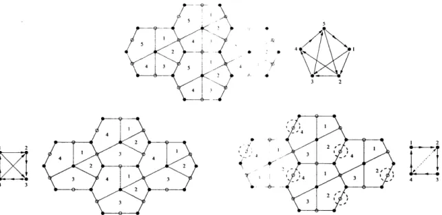
3.7.2 Pseudo del Pezzo 5 . . . . 80
4 Equivalence of algorithms
4.1 Introduction ... ... ...
4.2 Toric quivers and brane tilings . . . . 4.2.1 Geometry of the tiling embedding from conformal invariance . 4.2.2 Height function . . . . 4.3 Toric geometry from gauge theory . . . . 4.4 The conjecture . . . . 4.5 T he proof . . . . 4.5.1 Solving F-term conditions: gauge transformations and
mag-netic coordinates . . . . 4.5.2 The GLSM fields are perfect matchings . . . . 4.5.3 Height changes as positions in a toric diagram . . . . 4.6 Conclusions . . . . 5 Infinite families of examples
5.1 Introduction . . . . 5.2 Quiver content from toric geometry
5.2.1 General geometrical set-up . 5.2.2 Quantum numbers of fields.
5.3 The La,b,c toric singularities . .
5.3.1 The sub-family Laa . . . .
5.3.2 Quantum numbers of fields . 5.3.3 The geometry . . . . 5.4 Superpotential and gauge groups
5.4.1 The superpotential . . . . . 5.4.2 The gauge groups . . . . 5.5 R-charges from a-maximization . . 5.6 Constructing the gauge theories usir 5.6.1 Seiberg duality and transfor 5.6.2 Explicit examples . . . . 121 . . . . 121 . . . . 124 . . . . 124 . . . . 127 . . 136 . . . . 140 . . . . 141 . . . . 143 . . . . 149 . . . . 149 . . . . 150 . . . . 152 g brane tilings . . . . 154
aations of the tiling . . . . 156
. . . . 157 93 93 94 98 99 101 105 107 108 111 115 118
5.7 Conclusions. . . . ... 5.8 Appendix: More examples ...
5.8.1 Brane tiling and quiver for L 2 5.8.2 Brane tiling and quiver for L 6 Fast Inverse Algorithm
6.1 Superconformal fixed point and R-charges 6.2 Isoradial embeddings and R-charges.... 6.3 Rhombus loops and zig-zag paths . . . .
6.3.1 Inconsistent theories . . . ... 6.3.2 Conjecture of (p, q)-legs and rhombus 6.3.3 Parameter space of a-maximization . 6.4 Fast Inverse Algorithm . . . .
6.4.1 C3 (.
= 4). . . . ... 6.4.2 Conifold . . . . 6.4.3 L 3 1 . . . .. . . . 6.4.4 L 2 . . . . . 6.5 Toric duality and Seiberg duality . . ....
. . . . 165 . . . 166 . . . . 166 . . . . 167 169 169 .. . . . . 171 . . . 175 .. . . . . 177 loops . . . . 181 . . . . . 184 . . . 187 .. . . . . 187 . . . 190 . . . . . 192 .194 . . . . . 195
6.5.1 Seiberg duality in the hexagonal lattice with extra line 7 Exceptional Collections
7.1 Introduction... .. . . . . . . .. 7.2 Exceptional collections... . . . . . . . . ..
7.2.1 From Exceptional Collection to Periodic Quiver . . . .
7.2.2 Line Bundles and Curvature Forms for Toric Surfaces . 7.2.3 Bundles on P2 . . . . 7.2.4 Constructing the Quiver in General . . . . 7.2.5 Vanishing Euler Character.. . . . . . . . .. 7.3 Compatibility... . . . . . . ..
7.3.1 Beilinson quivers and internal matchings . . . . 7.3.2 Line bundles from tiling: The I-map . . . .
197 201 201 203 205 208 212 214 217 218 219 222
7.3.3 Reconstructing the quiver . . . . 7.4 Conclusions... . . . . . . . . . . . . ..
III Global geometry
8 Semi-flat spaces 8.1 Introduction . . . . 8.2 Semi-flat limit . . . . 8.2.1 One dimension 8.2.2 Two dimensions 8.2.3 Three dimensions 8.2.4 Flat vertices . . . 245 . . . 245 . . . 249 . . . 24 9 . . . 250 . . . 256 . . . 26 1 9 Non-geometric spaces 9.1 Stringy monodromies . . . . . . .. 9.1.1 Reduction to seven dimensions . 9.1.2 The perturbative duality group9.1.3 Embedding SL(2)2 in SL(4) . . . . 9.1.4 U-duality and G2 manifolds ..
9.2 Compactifications with D4 singularities 9.2.1 Modified K3 x T . . . . 9.2.2 Non-geometric T6/Z
2 x Z2 . . . . .
9.2.3 Asymmetric orbifolds . ... 9.2.4 Joyce manifolds . . . . ...
9.2.5 Dualities between models . . . . 9.2.6 U-duality and affine monodromies 9.3 Compactifications with E, singularities .
9.3.1 Orbifold limits of K3 . . . . 9.3.2 Example: T6/Z3 . . . . 9.3.3 Example: T6
/A12
. . . . 9.3.4 Example: T6/(Z2) 2 x Z4 265 . . . . 265 . . . . . . . . . . . . . . . 2 6 6 . . . . 2 6 9 . . . 2 72 . . . 2 76 . . . 2 78 . . . 2 78 . . . 28 0 . . . . 2 8 1 . . . 2 8 4 . . . 2 9 0 . . . 2 9 2 . . . 2 9 3 . . . 2 9 3 . . . 2 9 5 . . . 2 9 7 . . . . 2 9 7 228 238244
.9.3.5 Example: T6/A 24 . . . . 298
9.3.6 Non-geometric modifications . . . . 299
9.4 Chiral Scherk-Schwarz reduction. . . . . . . . 301
9.4.1 One dimension... . . . . . . . . . .. 301
9.4.2 Two dimensions... . . . . . . . 302
9.5 Conclusions . . . . 306
9.6 Appendix: Flat-torus reduction of type IIA to seven dimensions . . . 308
9.7 Appendix: Semi-flat vs. exact solutions . . . . 310
9.8 Appendix: The Hanany-Witten effect from the semiflat approximation 315 9.9 Appendix: Type IIA on T5/Z2 and Type IIB on S' x K3 . . . . 318
9.10 Appendix: List of asymmetric orbifolds . . . . 322
9.11 Appendix: Spectrum of T6/Z2 X Z2 and the two-plaquette model . . 325
9.12 Appendix: Spectrum of the one-plaquette model . . . . 331
9.13 Appendix: Spectra of Joyce orbifolds . . . . 334
List of Figures
1-1 D3-branes probing the transverse geometry... . . . . ... 38 1-2 Quiver of dP1. The theory contains four U(N) gauge groups labeled
by the nodes of the quiver. The arrows label bifundamental fields transforming in the (anti-)fundamental representation of the groups at the endpoints.. . . . . . . . . 39 1-3 dPi Beilinson quiver. . . . . 40
2-1 The cone for the variety. The coordinates of the spanning vectors are integers. The endpoints are coplanar following from the Calabi-Yau condition... . . . . . . . . . 42 2-2 The toric diagram for the conifold which can also be described by the
equation ziz2 = z3z4 with zi E C. The normal vectors are also shown. 44
2-3 The toric diagram for the del Pezzo 1 surface is shown. . . . . 44 2-4 The toric diagram for Li,7,3 which is part of the recently discovered
series of Lab, metrics ([61, 60]). . . . . 44
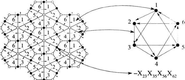
3-1 A finite region in the infinite brane tiling and quiver diagram for Model I of dP3. We indicate the correspondence between: gauge groups + faces, bifundamental fields +-+ edges and superpotential terms +-+ nodes. 50
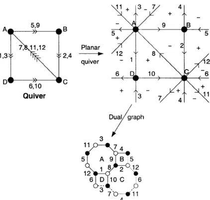
3-3 The quiver gauge theory associated to one of the toric phases of the cone over FO. In the upper right the quiver and superpotential (3.0.6) are combined into the periodic quiver defined on T2. The terms in the
superpotential bound the faces of the periodic quiver, and the signs are indicated and have the dual-bipartite property that all adjacent faces have opposite sign. To get the bottom picture, we take the planar dual graph and indicate the bipartite property of this graph by coloring the vertices alternately. The dashed lines indicate edges of the graph that
are duplicated by the periodicity of the torus. This defines the brane
tiling associated to this M = 1 gauge theory. . . . . 52
3-4 a) Brane tiling for Model I of dP3 with flux lines indicated in red. b) Unit cell for Model I of dP3. We show the edges connecting to images of the fundamental nodes in green. We also indicate the signs associated to each edge as well as the powers of w and z corresponding to crossing flux lines. . . . . 55
3-5 Toric diagram for Model I of dP3 derived from the characteristic poly-nom ial in (3.1.10). . . . . 56
3-6 F-term equations from the brane tiling perspective. . . . . 60
3-7 Quiver diagram for the SPP. . . . . 61
3-8 Brane tiling for the SPP. . . . . 61
3-9 Toric diagram for the SPP. We indicate the perfect matchings corre-sponding to each node in the toric diagram. . . . . 62
3-10 Perfect matchings for the SPP. We indicate the slopes (hW, hz), which allow the identification of the corresponding node in the toric diagram as shown in Figure 3-9. . . . . 63 3-11 Integrating out a massive field corresponds to collapsing the two
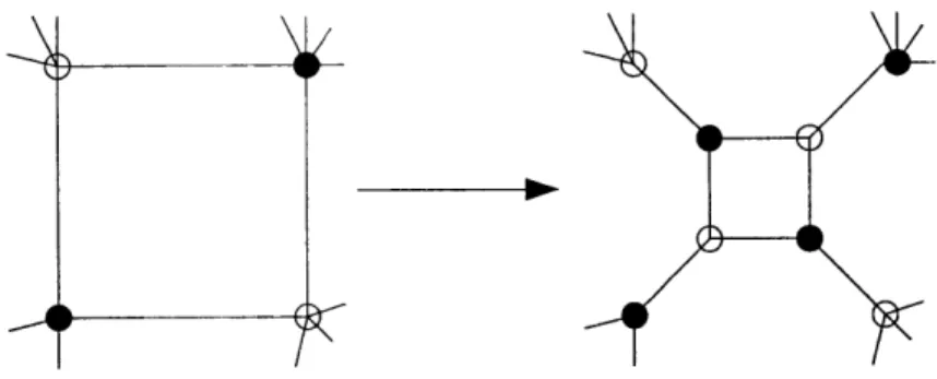
3-12 The action of Seiberg duality on a periodic quiver to produce another toric phase of the quiver. Also marked are the signs of superpotential terms, showing that the new terms (faces) are consistent with the
pre-existing 2-coloring of the global graph. . . . . 68
3-13 Seiberg duality acting on a brane tiling to produce another toric phase. This is the planar dual to the operation depicted in Figure 3-12. When-ever 2-valent nodes are generated by this transformation, the corre-sponding massive fields can be integrated out as explained in Section 3 .3 . . . . 69
3-14 The operation of Seiberg duality on a phase of FO. . . . . 69
3-15 Removing the edge from between faces 5 and 6 Higgses Model I of dP3 (top) to one of the two toric phases of dP2 (bottom). . . . . 71
3-16 The dP2 tiling (top) can be taken to either dP1 (bottom left) or Fo (bottom right), depending on which edge gets removed. In the FO tiling, one should collapse the edge between regions 2 and 4 to a point; this corresponds to the bifundamentals on the diagonal of the quiver. 72 3-17 Quiver diagram admitting two toric superpotentials. . . . . 73
3-18 Brane tiling corresponding to the quiver diagram in Figure 3-17 and the superpotential in (3.6.28). . . . . 74
3-19 Brane tiling corresponding to the quiver diagram in Figure 3-17 and the superpotential in (3.6.29).. . . . . . . . . 74
3-20 Toric diagram for the quiver in Figure 3-17 and superpotentials WA andWB . . . . . . .. - - - - .... . . . . ... - .. . 75
3-21 Brane tiling for Model I of dP2. . . .. . . . . 76
3-22 Brane tiling for Model II of dP2. . . . . 76
3-23 Brane tiling for Model III of dP3. . . - .. . . . . . . - - - - -. . . 77
3-24 Brane tiling for Model IV of dP3. . . . 78
3-26 Toric diagrams with multipl( it hir the four toric phases of PdP5.
We observe that the GLSM linit iplicities are the same for Models I
and III. ... .... .... ... ... 82
3-27 Brane tiling for Y3,3 . . . .. 83
3-28 Brane tiling for Y3 ,2. The inpurit v is the blue area. . . . . 83
3-29 Brane tiling for Y3,1. . . . .. 84
3-30 Toric diagram of a phase ofY . . . .. 86
3-31 Toric diagram of a phase of Y4'" with three single impurities. . . . . . 87
3-32 Dualizing face 3 in Y3,1 with two single impurities. In resulting tiling, we indicate the double impurity in pink.. . . . .. 88
3-33 The double impurity in Y3 . . . . 88
3-34 Toric diagram for Y3,1 in the double impurity phase . . . . 89
3-35 Brane tilings for y3,q. . . . . 90
3-36 A brane tiling for X 3,1. . . . 90
4-1 Quiver diagram for Model II of dP. . . . . 95
4-2 Periodic quiver for Model II of dP2. We show several fundamental cells. 95 4-3 Two plaquettes are equal once the F-term equation for the common field is imposed... . . . . . . . .. 96
4-4 Brane tiling for Model II of dP2. . . . 98
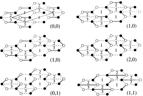
4-5 (a) The dimers in the a perfect matching M are shown in cyan. (b) The dimers in the reference perfect, matching Mo are shown in red. (c) The height function, whose level curves are given by M - Mo. .... 99
4-6 Relevant matrices in the Forward Algorithm. . . . . 105
4-7 Contours defining i', and f9y. ... 111ill. 4-8 Sets of edges E., and Ey that enter the computation of (hr, hy). . . . 116
4-9 Perfect matchings and their slopes for Model II of dP2. . . . 119
5-1 A four-faceted polyhedral cone in R3. . . . 125
5-2 Toric diagram for the La,5,A geometries. . . . . 138
5-4 a) Toric diagram and b) (p, q) web for the Lo'b'" sub-family. . . . . . 141
5-5 The four building blocks for the construction of brane tilings for La'b'c 155 5-6 Seiberg duality on a self-dual node that does not change the hexagon content. . . . . 157
5-7 Seiberg duality on a self-dual node under which (nA, nB, InC, nD) -+ (nA + 1, nB - 2, nc, nD + 1)- . . . . - - - -... - 157
5-8 Brane tiling for L2 3. . . . 158
5-9 Quiver diagram for L263. . . . . 159
5-10 Toric diagram for L2'6,3 determined using the characteristic polynomial of the Kasteleyn matrix for the tiling in Figure 5-8. . . . . 160
5-11 Brane tiling for a Seiberg dual phase of L2 3. . . . . 160
5-12 Brane tiling for L2 4. . . . 161
5-13 Brane tiling for L2 4. . . . 161
5-14 Brane tiling for L '. . . . . 164
5-15 Quiver diagram for La,,a. It consists of 2a C nodes and (b-a) A nodes. The last node is connected to the first one by a bidirectional arrow. 164 5-16 Brane tiling for L' 2. . . . 166
5-17 Quiver diagram for Li, 2. . . . . 166
5-18 Toric diagram for L' 2. . . . . 167
5-19 Brane tiling for L1'7 3. . . . 167
5-20
Quiver
diagram for L1,7,3. . . . . 1685-21 Toric diagram for L 73. . . . . 168
6-1 Isoradially embedded part of an arbitrary brane tiling (in green). . . . 172
6-2 (i) Circumcircles around the faces (in black), (ii) and the corresponding rhombus lattice (in red). . . . . 172
6-3 A rhombus in the lattice. The green line is an edge in the brane tiling, the magenta line is the corresponding bifundamental field in the periodic quiver. . . . . 173
6-4 (i) Rhombus path in the rhombus lattice. (ii) Equivalunt ig -zag path in the brane tiling. We will use blue lines to depic rhombus loops schematically. The edges which are crossed by Ihe blue line in (i) are all parallel. Their orientation can be described by an angle, the so-called rhombus loop angle. . . . . 175 6-5 Tilting along the horizontal R rhombus loop. The rhombus loop angle
a changes during the Dehn-twist. Here we have chosen ( = 0 to be the vertical direction
(1),
hence a = 7r/4 corresponds to the skew edges(/)...
. . . .
. . . 176
6-6 Hirzebruch zero brane tiling.... . . . . . . . 178 6-7 (i) Hirzebruch zero toric diagram (ii) un-Higgsed Hirzebruch. The arearemains the same, external multiplicities appear. . . . . 178 6-8 (i) Hirzebruch zero toric diagram (ii) un-Higgsed Hirzebruch. The area
increases by 1/2 corresponding to the new face in the brane tiling. . . 179
6-9 (i) Hirzebruch zero inconsistently un-Higgsed. (ii) Consistent un-Higgsing... . . . . . . . 179 6-10 (i) Inconsistently un-Higgsed Hirzebruch. The rhombus loops are
indi-cated with the blue lines. The zig-zag paths contain the edges that are crossed by the blue paths. The following rhombus loops are obtained: A : (0, -1) B : (-2, 2) C : (2, -1). Here (a, b) denotes the homology class of the path.
(ii) Consistently un-Higgsed FO. The rhombus loops reproduce the (p, q)-legs of the toric diagram (Figures 6, 7): A : (0, -1) B : (0, 1)
C : (-2, 1) D : (1, -1) E : (1, 0). . . . . 180 6-11 The subgraph connects to the rest of the tiling through its four nodes
in the corner. No consistent brane tiling can contain this subgraph,
6-12 Toric diagram (i) and (p, q) -web (ii) for del Pezzo 2. The charges of the external branes are shown. According to the conjecture, these correspond to the homology classes of the rhombus loops in the brane tilin g . . . . . 182 6-13 Toric diagram for the SPP. We have drawn the blue (p, q)-leg between
the nodes (1, 1) and (2, 0). The zig-zag path corresponding to the leg is shown in Figure 19. . . . . 183 6-14 The six periodic perfect matchings of SPP [94]. The green edges are
contained in the matching, the dashed lines are the other edges of the tiling. The (s, t) numbers are the corresponding points in the toric
diagram (Figure 17). . . . . 184 6-15 The (1, 1) and (2, 0) perfect matchings on top of each other. We see
the emerging (1, 1) homology zig-zag loop which corresponds to the blue (p, q)-leg in Figure 17. . . . . 185 6-16 PdP4 model I brane tiling with a (1,0,1,0,1,0,0)
Nf
= 2 fractional brane[98]. The bounding rhombus loops (A and B zig-zag paths) are shown in blue... . . . . . . . . 186 6-17 Assigning angles (6) to the rhombus loops. The figure shows two
in-tersecting blue rhombus paths. There is a single rhombus and a green bifundamental edge at the intersection of these paths. This bifun-damental has an R-charge that is proportional to the angle 6 of the rhombus. This angle is just the difference of the rhombus loop angles a and / assigned to the two rhombus paths: R7 = 0 =
|a
-#1
(or7r -
la
-#1
depending on the orientation). . . . . 187 6-18 C3 toric diagram . . . . 1886-19 Rhombus loop diagram of C3. The blue rhombus loops are the D6-branes. At the intersection points we get massless fields. The dark faces are terms in the superpotential, the light faces are the gauge groups. These correspond respectively to nodes and faces in the brane tiling. The rhombi are shown in red, the brane tiling edges are green. 188
6-20 From the rhombi to the brane tiling. We glue the rhombi together that arise at the intersections of rhombus loops (Figure 27). We glue the edges that are connected by the rhombus loops. Each rhombus has a green tiling edge in it, from which we obtain the entire (hexagonal)
brane tiling. . . . . 189
6-21 Conifold toric diagram . . . . 190
6-22 Conifold rhombus loops and brane tiling . . . . 190
6-23 Four fundamental cells of the conifold rhombus loop diagram. If we consider these cells as one big fundamental cell then we gain the rhom-bus loop diagram of the Z2 x Z2 orbifold of the conifold. . . . . 191
6-24 Z2 x Z2 orbifold of the conifold. . . . . 191
6-25 L"' toric diagram . . . . 192
6-26 L13' rhombus loops and brane tiling . . . . 192
6-27 (i) L13 ' brane tiling (ii) and the corresponding quiver. . . . . 193
6-28 Toric diagram of L. 2 . . . . . . . . . . . . . . . . . . . . . . . . 194
6-29 L152 brane tiling from the rhombus loops . . . . 195
6-30 2 x 2 fundamental cells of the rhombus loop diagram of L152. The brane tiling is shown in green. . . . . 196
6-31 (i) Li52 brane tiling (ii) and the corresponding quiver . . . . 197
6-32 The elementary Picard-Lefschetz-Yang-Baxter transformation. . . . 197
6-33 The Yang-Baxter-Reidemeister transformation on the rhombus lattice. Star-triangle . . . . 198
6-34 (i) Four hexagon with one extra line. (ii) Seiberg dualizing the red square (F). The extra edge in the upper hexagon (B & F) gets into the lower one (F & C). . . . . 198
6-35 Seiberg duality in the hexagonal tiling with extra edge. The brane tiling is shown in green, the (deformed) rhombus lattice is in red, the relevant rhombus loops are in blue. . . . . 199
7-1 Four unit cells of the P2 periodic quiver for basepoint (XI, x
2) = (3/4, -1/2).214
7-2 The periodic Beilinson quiver for dP1 with fundamental cell. . . . . . 216
7-3 The eight periodic perfect matchings of dP1. The green edges are contained in the matching. The dashed lines are the edges left in the tiling. The (s, t) numbers are the corresponding points in the toric
diagram... . . . . . . . . . 219 7-4 Allowed face paths (i.e. paths in the Beilinson quiver) go always uphill.
The height function increases by one at the line constituted of the black perfect matching and the green reference matching. The red path cannot cross the green edges (they are not in the Beilinson quiver). Hence when crossing the contour line, the red path has to cross a black edge. Crossing the black edge increases the value of the height function.222 7-5 Gradient vectors in the toric diagram. The coordinates of the blue
(si, ti) vectors give the monodromy of the height function of the perfect matching sitting at their endpoints. The red (x, y) arrow is the gradient vector of the hypothetical nontrivial loop. . . . . 222 7-6 An integer function over the external nodes determines a divisor and
therefore a sheaf of sections of the corresponding line bundle. The numbers in the figure denote O(D1
+
D3 + 2D4). . . . . 2237-7 The I-m ap. . . . . 223 7-8 The reference paths are allowed paths to each face. They start from
face 1 and don't cross the edges of the green internal matching; hence they are paths in the Beilinson quiver. . . . . 225 7-9 The three divisors computed from the paths to the faces. . . . . 226 7-10 Face 4 can be assigned with either the red or the yellow allowed path.
The resulting Weil divisors are shown on the right-hand side. We see that they differ by a linear function, i.e. they are equivalent. . . . . . 226
t t I [) ermining the S2,4 matrix element. In this case E4 E*L = (1, 0, 1, 1)-(. 0. 0, 0) = (0, 0, 1, 1). The figure shows the lattice of t he A2,4 polygon
andI its bounding inequalities. The red lattice points inside A2,4 can
be identified with adjacent fundamental cells in the brane tiling. . . 229
7-12 The figure shows the allowed paths that start on face 2 and end on faice 4. The endpoints of these paths are in different fundamental cells which are in one-to-one correspondence with the lattice points inside
A24 that has been used to compute dim Hom(E2, E4). . . . . 230
7-13 The F-flatness equation for the X bifundamental field is CBA = VU.
This states the equivalence of the two green paths in the figure. . . . 231
7-14 Homotopic paths are equivalent. The left-hand side of the figure shows two paths represented schematically by green lines. The tiling is col-ored black and the underlying rhombus lattice is shown by dotted lines. The pink area surrounded by the two paths is also shown separately. 231
7-15 Two homotopic paths that pass around the pink area. Each boundary
node (A1, . .., An, B1, ... , Bin) has at least one rhombus edge which
ensures that the area cannot be reduced by F-terms. . . . . 232
7-16 The straight rhombus path in the area contains rhombi ro, ... , r,. The
existence of this series of rhombi constrains AB1 to be parallel to BmB. 232
7-17 The embedding of the dual cone in the tiling torus. . . . . 233
7-18 Inequivalent A --+ B homotopic paths in an inconsistent tiling. . . . 234
7-19 Homotopic paths with different R-charge are not equivalent. After applying the F-term equation for A3B1, the long path (solid green
line) gets transformed to the short path (dashed line) plus a small loop around the Ai node in the tiling. . . . . 235
7-20 The figure schematically depicts three allowed green paths from A to
B. The shading indicates one of the height coordinates. The height
increases in the direction of the small arrows. The allowed paths can only cross the dashed lines in this direction, and thus we obtain a bounding inequality for AAB. The remaining edges can be determined by means of the other heights... . . . . . . . . 236 7-21 Y 3,2 quiver. . . . . 240 7-22 Y3,2 perfect matchings (1st ...
9th) . . . . .. 241
7-23 Y3
,2 perfect matchings (1oth... 18th) . . . . .. 242 7-24 Y3,2 Beilinson quiver. Bifundamentals in internal matching 7 are omitted. 242 7-25 Y3,2 tiling. The purple lines indicate the chosen paths that are used
to compute the exceptional collections. The paths start on face 1 and connect it to the other faces. . . . . 243 7-26 A set of reference paths for Y3
,2. . . . . 243
8-1 A possible fundamental domain (gray area) for the action of the SL(2, Z) modular group on the upper half-plane. The upper-half plane parametrizes the possible values of r (or p): the moduli of a two-torus. The gray domain can be folded into an S2 with three special points (the two orbifold points: TZ, - e27"'6 and Tz4 = i, and the decompactification
point: T -+ ioo). . . . . 250
8-2 Base of the T4/Z 2 orbifold. The Z2 action inverts the base coordinates
and has four fixed points denoted by red stars. They have 180' deficit angle. As the arrows show, one has to fold the diagram and this gives an S2
. . . .. . . . . . .. . . . . .. . . . . .. 255 8-3 Flat S2 base constructed from four triangles: base of K3 in the Z2
8-4 Singularities in the base of T6/Z 2 x Z2. The big dashed cube is the
original T3 base. The orbifold group generates the singular lines as depicted in the figure. The red dots show the intersection points of these edges. ... ... 257 8-5 (i) Rhombic dodecahedron: fundamental domain for the base of T6/Z2 x
Z2. Six pyramids are glued on top of the faces of a cube. Neighbor-ing pyramid triangles give rhombi since the vertices are coplanar (e.g. ABCD). (ii) The S3 base can be constructed by identifying triangles
as shown by the arrows. After gluing, the deficit angle around cube edges is 1800 which is appropriate for a D4 singularity. The dihedral
angles of the dashed lines are 1200 and since three of them are glued to-gether, there is no deficit angle. The tips of the pyramids get identified
and the space finally becomes an S3. . . . . 259
8-6 The base of T6/Z2 x Z2 is homeomorphic to a three-ball with an S2
boundary which has to be folded as shown in the figure . . . 260 8-7 Monodromies for the edges. . . . 260 8-8 The solid angle at the apex is determined by the dihedral angles
be-tween the planes. . . . 261 8-9 Flat vertex. A, B and C are singular edges. C is pointing towards the
reader. The dashed lines must be glued together to account for the deficit angle around C. . . . . 262 8-10 Junction condition for monodromies. The red loop around A can be
smoothly deformed into two loops around B and C. . . . 262
9-1 Almost non-geometric T6/Z
2 x Z2 spaces. Monodromies are modified
along the red loops. We refer to the models as one-plaquette, two-plaquette, "L", "U" and "X", respectively. . . . . 281
9-3 (i) Fundamental d(main of the base after modding by Y: half of a
rhombic dodecahedron. The arrows show how the faces are identified. (ii) Schematic picture indicating the structure of the degenerations. . 287 9-4 (i) Half of the fundamental domain after modding by -Y. (ii) Schematic
picture... . . . . . . . 288 9-5 The base of T'/(Z2)2 where the generators of Z 2's include coordinate
shifts. Four non-intersecting D4 strings (dashed green lines in the
middle of hexagons) curve the space into an S3. See the figure in Appendix 9.13 for a pattern that can be cut out . . . . 288 9-6 (i) The base can be constructed by gluing the truncated tetrahedron
(dashed lines) to itself along with a small tetrahedron. It is easy to check that the D4 strings (solid lines) have 1800 deficit angle whereas
the dashed lines are non-singular. (ii) Schematic picture. The trun-cated tetrahedron example can roughly be understood as four linked rings of D4 singularities. All of the rings are penetrated by two other
rings which curve the space into a cylinder as they have tension 12. This forces the string to come back to itself. . . . . 289 9-7 (i) The base of the
( ,
j, j)
Joyce orbifold. There are six strings locatedon the faces of a cube. These faces are folded up which generates the 180' deficit angles. (ii) Schematic picture. The degenerations form three rings of D4 singularities. . . . . 289
9-8 Monodromies of the one-shift Joyce orbifold. . . . . 290 9-9 The base of the T4/Z
3 orbifold contains three E6 singularities. . . . 294
9-10 The base of the T4/Z
4 orbifold contains two E7 and one D4
singulari-ties. . . . . 295 9-11 The base of the T4/Z
6 orbifold contains E8, E6 and D4 singularities.
9-12 The base of T6/Z3. The green line shows the E6 singularity. Six trian-gles bound the domain. Two triantrian-gles touching the singular green line are identified by folding. Two triangles should be identified according to the orientation given by the arrows. The remaining two triangles are identified in a similar fashion. . . . 296
9-13 (i) The base of T'/A1 2. The red and green lines indicate E6, D4
sin-gularities, respectively. The other edges are non-singular. The solid green cube indicates the D4 singularities of the original T6/ (Z2)2 orb-ifold. (ii) Schematic picture describing the topology of the singular lines. See Appendix 9.14 for building this polyhedron at home. . . . . 298
9-14 (i) The base of T6/ (Z
2)2 x Z4. The red and green lines indicate E7,
D4 singularities, respectively. The other edges are non-singular. The
solid green cube indicates the D4 singularities of the original T6/ (2) 2
orbifold. (ii) Schematic picture describing the topology of the singular lines. . . . . 299
9-15 (i) The base of T6/A
2 4. The cyan, red and green lines indicate E7,
E6 and D4 singularities, respectively. (ii) Schematic picture describing
the topology of the singular lines. . . . . 300
9-16 Non-geometric T6/A 12. The red lines indicate extra (-l)FL factors. . 301
9-17 Non-geometric T6/(Z 2)2 x Z4. . . . . 301
9-18 Non-geometric T6
/A
24. . . . . 3029-19 Fundamental domain (gray area) for the action of the Fo(2) on the upper half-plane. . . . ... 304
9-20 (i) Comparing semi-flat and exact metrics for around degenerating fibers. The base is 3d, parametrized by the periodic x coordinate and the complex z-plane. The red line
/
red dots indicate where the S' fiber vanishes. Translational invariance of the semi-flat solution is replaced by periodicity of the exact metric in the x direction. (ii) The same (exact) metric from a different viewpoint. The horizontal direction in the torus fiber is the x coordinate. The torus pinches at the degeneration point (red dot) in the 2d base. Topologically, the singular fiber is an S2 with two points glued together. This replacesthe degenerating T2 -+ oc torus of the semi-flat solution. . . . . 314
9-21 Hanany-Witten brane creation mechanism. A and B are the mon-odromies of the NS5- and D6-branes, respectively. As the two branes pass through each other, a new brane appears with a monodromy around the green circle (see right-hand side). This monodromy can be easily computed in the original configuration (left-hand side) where the green path was a deformed loop around the two branes. The result is ABA- 1B-1 which is simply the monodromy of a D4-brane. . . . . 316 9-22 Determining the monodromy around the green loop by means of 2d
branch cuts. ... ... 317 9-23 T5
/Z
2 as a fibration over S2. The geometric T3 fiber gets promotedto T' by adding x" and the M-theory circle x". The monodromy M then acts on this T . . . . 319 9-24 Almost non-geometric T6/Z 2 x Z2 which is also a Joyce orbifold. It is
T-dual to T6/Z2 X Z2. . . . . 322
9-25 This modified T6/Z 2 x Z2 is also a Joyce manifold. . . . . 323
9-26 Truncated tetrahedron: the shifted T6/Z 2 x Z2. . . . . 338
9-27 Rhombic dodecahedron: fundamental domain of T6/Z
2 X Z2. . . . . . 339
List of Tables
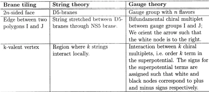
3.1 Dictionary for translating between brane tiling, string theory and gauge theory objects. . . . . 47 5.1 Charge assignments for the six different types of fields present in the
general quiver diagram for La . . . . 143
8.1 Examples for composite vertices. . . . . 263 9.1 The two basic representations of the duality group. . . . . 269 9.2 Some well-known examples for the Gibbons-Hawking ansatz. . . . . . 313 9.3 Branes in the Hanany-Witten setup. 456 are the base, 789 are the fiber
coordinates.. . . . . . . . . 315 9.4 Massless M = 2 multiplets in four dimensions (Weyl fermions and real
scalars). . . . . 325 9.5 Untwisted NS and R sectors. In the R sector, only the spins of compact
complex dimensions are indicated. The remaining one is determined
by the GSO projection as indicated by the "gso" label. This depends
on whether it's the left or right R sector. . . . . 326 9.6 Untwisted sectors. The signs show the matter GSO projection (which,
due to the superghost contributions, differ from the full GSO in the N S sectors). . . . . 326 9.7 (ao)-twisted NS and R sectors. The other twisted sectors are
analo-gous. The dots indicate half-integer moded oscillators which generate m assive states. . . . . 327
9.8 Each twisted sector gives an M= 2 vector multiplet. . . . 327 9.9 Massless A = 1 multiplets in four dimensions (Weyl fermions and real
scalars). . . . 328 9.10 Signs of projections in various twisted sectors. . . . 329 9.11 Assignment of signs for discrete torsion . . . 329 9.12 -twisted NS and R sectors. . . . 329 9.13 (a)-twisted NS and R sectors. . . . 331 9.14 Assignment of phases for the twisted sectors (columns). Dots indicate
signs that do not affect the spectrum calculation. The group elements that are not listed here have no non-trivial fixed loci. . . . 332 9.15 Untwisted closed sectors. . . . 332 9.16 a-twisted sector: a chiral multiplet. . . . 333 9.17 Twisted sector: a vector and a chiral multiplet. . . . 333 9.18 Twisted sectors that include (-1)FL: two chiral multiplets. The
left-moving GSO projections are modified compared to the usual twisted sectors. . . . 333 9.19 Twisted sectors for (bi, b2, c1, c3, c5) = (0, 1 2' 2' 2'1, i, 0, 0) give a vector and
Part I
Our current understanding of Nature is centered around two theories: general relativity which describes gravity, and quantum field theory which describes the strong and electroweak interactions and various low-energy phenomena. Naive attempts to unify these two theories lead to insurmountable difficulties. Moreover, a unified theory would ideally explain recent cosmological observations such as the acceleration of the universe, dark matter and cosmic inflation. This presents challenges to our understanding that must be addressed by new ideas.
As of today, the best candidate framework for unification is string theory. The best understood solutions of the theory are, however, ten dimensional. The extra six dimensions may be compactified. The various deformations of the compact space can lead to light moduli fields. Fields with flat potentials typically modify the gravita-tional law in a way which is experimentally ruled out. More generic states of string theory also contain field strengths and heavy solitonic objects, branes, which can generate a potential for the moduli fields. It is in fact possible to fix all the moduli in particular examples. There is expected to exist a large set of consistent string theory vacua which is referred to as the 'landscape'. It is important to study the properties of these vacua through examples and determine possible correlations between their features. It is conceivable that this way one can obtain predictions for low-energy physics and constrain the set of effective field theories.
After compactifying, the structure of the extra dimensions governs the particle content and interactions of the four-dimensional effective field theory. Much of the work in this thesis has focused on this interesting correspondence. In many cases, the basic features of the field theory depend only on the local structure of the extra dimensions. In this introduction, we briefly explain the results which fully solve this correspondence for the case of 'toric' geometries. The tools that we developed can also be used to generalize the recent discoveries for M2-branes in M-theory. Finally, we describe results in global compactifications, in particular, in constructing 4d
N
= 1 perturbative non-geometric backgrounds. Global issues are of importance since certain mechanisms (e.g. inflation) can depend on the structure of the entire compact space.Local geometries and singularities
A popular scenario for phenomenology describes visible particles as excitations of three-dimensional branes. In order to generate the chiral particle content of the Standard Model in Type II string theory, the compact space must contain singularities (or intersecting branes in a dual picture) where the branes are placed. Although general relativity breaks down in the presence of such singularities, string theory can still be well-defined [73, 71]. The data for specifying the low-energy effective theory on the brane include the superpotential and the quiver which encodes the gauge groups and the particle content. These features depend only on the local region near the singularity.
The existing methods for analyzing the correspondence were computationally pro-hibitive for most singularities. For Calabi-Yau geometries with toric symmetries, we introduced "brane tilings" which efficiently solved this problem in a graphical way [94]. This paper is the basis of Chapter 3. The tiling can be interpreted as a physical configuration of branes. It encodes the gauge group, matter content and superpoten-tial of the gauge theory. Brane tilings give the largest class of K = 1 quiver gauge theories yet studied and they offer a generalization of the AdS5/CFT 4 correspondence to infinite sets of non-spherical horizons.
The technique we developed also enabled one to quickly compute the toric vacuum moduli space of the quiver gauge theory. In [100], we explicitly proved the equivalence between this procedure and the earlier approach that used gauged linear sigma models
[232]. This is summarized in Chapter 4.
As an application of brane tilings, in [97] we found the four dimensional quiver gauge theories that are AdS/CFT dual to the recently discovered La',b, families of 5d Sasaki-Einstein metrics. Chapter 5 is based on this paper. We perform various checks of the correspondence, such as volume calculations on the string side which match the R-charges on the gauge theory side which are determined by a-maximization.
In [132], we developed a procedure that constructs the brane tiling for any toric Calabi-Yau threefold. This is summarized in Chapter 6. The algorithm solved a
longstanding problem by computing superpotentials for these theories directly from the toric diagram of the singularity. The rules for the consistency of tilings were also determined. In general, the correspondence between field theories and geometries is not one-to-one: various field theories can have the same moduli space. This ambiguity manifests itself as Seiberg duality which was further elucidated by the results.
Brane tilings give a simple pictorial way to determine the low energy gauge theory on a stack of D3-branes probing a toric singularity. Another more abstract approach to this problem uses so-called exceptional collections of sheaves associated to the base of the threefold. Although this method is not restricted to the toric case, it
is considerably more complicated. In [125] we provided a dictionary that translates between these two languages. These results are described in Chapter 7.
In order to gain a better understanding of the field theory
/
geometry correspon-dence, in [51] we discussed in detail the problem of counting BPS gauge invariant operators in the chiral ring of quiver gauge theories. These operators are dual to generalized giant gravitons, i.e. D3-branes wrapped on generically nontrivial three-cycles on the gravity side. We found an intriguing relation between a certain decom-position of the generating function and the discretized Kdhler moduli space of the Calabi-Yau space.In [95] we developed techniques for orientifolding toric Calabi-Yau singularities. With these new tools, one recovers many orientifolded theories known so far. Fur-thermore, new orientifolds of non-orbifold toric singularities were obtained. One particular application of the results is the construction of models which feature dy-namical supersymmetry breaking as well as the computation of instanton induced superpotential terms.
As discovered recently, Chern-Simons-matter theories play a role in M-theory [210, 20, 21, 122]. In particular, they are conjectured to describe the 2+1 dimen-sional low-energy theory living on M2-branes. Understanding the physics of these branes will be a further important step towards understanding M-theory and non-perturbative strings. Brane tilings proved to be efficient tools for studying a subset of
N
= 2 Chern- Sinous-matter theories [135]. In[133],
we described a te( Iique which computes the three dimensional toric diagram of the non -compact imodili space of a single probe brane. As a byproduct, one obtained new examples for the AdS4/CFT 3 correspondence. These examples may be useful for the study of 2+1 (liniensional condensed matter systems.Global non-geometric compactifications
The study of geometric compactifications is possible due to the abundance of available mathematical tools. Such vacua, however, represent only a very small subclass of the
landscape: the generic vacua are non-geometric. The classification of such theories seems prohibitively difficult and therefore simple tractable examples are valuable. A first step can be made in a controlled environment using perturbative string dualities to build non-geometric spaces.
The second part of this thesis (Chapters 8-9) focuses on implementing these ideas to obtain four-dimensional M = 1 compactifications [229]. At the 'large complex structure point' in the moduli space, Calabi-Yau spaces can be approximated by torus fibrations [113, 220]. Instead of using only geometric SL(n) transformations to glue the torus fibers, one wishes to use the whole T-duality (or more ambitiously, U-duality) group [138]. The non-geometric spaces that we obtain this way have a nice geometric representation. The construction is dual to G2 compactifications of M-theory and has asymmetric orbifold limits. It also allows for new ways to stabilize the moduli fields. In particular, it is useful in eliminating the modulus that is related to the overall size of the compact manifold which otherwise poses an intrinsic difficulty for ordinary (geometric) string compactifications. We also give a simple explanation for the Hanany-Witten brane-creation mechanism [134] and for the equivalence of the T5/Z 2 Type IIA orientifold and Type IIB on S' x K3 [234, 67].
Part II
Chapter 1
D-branes and quiver gauge theories
String theory contains a wide variety of extended objects. In addition to 1+1-dimensional strings, it also contains branes, which are higher 1+1-dimensional analogs of two-dimensional membranes. There exist various types of branes1: NS5-branes, Dp-branes (in Type II string theory) and also M2- and M5-branes (in M-theory). In this first part of the thesis, we will focus on the physics of D-branes and how local features in the geometry affect their dynamics.
In perturbative string theory, D-branes are submanifolds in spacetime where strings can end. The effective action for a D-brane is given by the Dirac-Born-Infeld action coupled by a Wess-Zumino term to other spacetime fields [182]. One can consider a limit where the length scale of the strings vanishes and the massless modes on the D-brane decouple from the tower of massive open string modes and other modes arising from closed strings in the bulk of spacetime. For a single D-brane in flat space, the low-energy limit corresponds to the dimensional reduction of the ten-dimensional A = 1 supersymmetric Yang-Mills theory with U(1) gauge group.
Placing D-branes in curved background geometries offers an immediate general-ization to the flat space configuration. The following question arises naturally: for a given geometry, what field theory governs the low-energy dynamics of the D-branes? A possible approach to study this question, which is particularly interesting due to its relationship with different branches of geometry, is to use D-branes to probe
a >inigllarity in the geometry. The geometry of the singularity then determines the an oit of supersymmetry, the gauge group structure. the matter content and the siperpotential interactions on the worldvolume of the D-branes.
The richest of such examples which are both tractable and non-trivial, are given by t he 4d KV 1 gauge theories that arise on a stack of D3-branes probing a singular Calabi- Yau 3-fold. This scenario is depicted in Figure 1-1. The background is a product of (3+1)-dimensional Minkowski space and a six-dimensional Calabi-Yau space. The D3-branes are filling the Minkowski factor. Their position in the extra six dimensions is given by a point in the Calabi-Yau manifold. If this is a smooth point in the Calabi-Yau geometry, we obtain M = 4 SYM on the D-branes. However, if the point is a singular point, the low-energy theory of the D-branes will be more
interesting.
space-filling D3-branes
0 4
<
singular Calabi-Yau
Figure 1-1: D3-branes probing the transverse geometry.
This setup also provides generalizations of the celebrated AdS/CFT correspon-dence [189, 118, 236, 6]. The AdS/CFT conjecture states that the large N 't Hooft limit of K = 4 SU(N) super Yang-Mills is equivalent to type IIB string theory on AdS x S' with N units of Ramond-Ramond 5-form flux on the S'. The K = 4 gauge
theory in question arises as the worldvolume theory of a stack of N D3-branes in flat ten dimensional space. Since its original formulation, the AdS/CFT correspondence has been extended to and checked in a variety of more realistic, less supersymmetric situations. The worldvolume theory of D3-branes over a singular Calabi-Yau
reflects the properties of the singular manifold. When the Calabi-Yau is a metric cone over an X5 Sasaki -Eiiistein manifold, the corresponding dual is type IIB string
theory on AdS5 x X5.
The matter content of the quiver gauge theory is neatly summarized in the quiver graph
[73]
which also generalizes the familiar Dynkin diagrams. Each node in the quiver (see e.g. Figure 1-2) may carry an index, Ni, for the ith node and denotes a U(Nj) gauge group. The edges (arrows) label the chiral bifundamental multiplets. These fields transform in the fundamental representation of U(Nj) and in the anti-fundamental of U(Nj) where i andj
represent the nodes in the quiver that are the head and tail of the corresponding arrow.1
z
2
1 2
U"X Ua
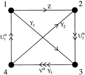
4
VaY 33
Figure 1-2: Quiver of dP1. The theory contains four U(N) gauge groups labeled by the nodes of the quiver. The arrows label bifundamental fields transforming in the (anti-)fundamental representation of the groups at the endpoints.
In order for the gauge theory to be gauge anomaly free, for each gauge group, the number of chiral fermions in the fundamental representation must equal the number in the antifundamental representation. This anomaly cancellation constraint means that for a fixed node in the quiver, the number of incoming and outgoing arrows are the same.
In order to write down the Lagrangian of the quiver gauge theory, we further need to give the superpotential, which is a polynomial in gauge invariant operators. For
example, for dP1 the superpotential is2
W =ea3U1VY1 - E1a/U 2Y2YS - 1YUZ .%-2U (1.0.1)
By deleting certain arrows in the quiver, one obtains another graph, the so-called Beilinson quiver. This type of quiver will be important in Chapter 7. In this quiver there exists an ordering of the nodes such that there are no arrows pointing backwards (for an example see Figure 1-3). Generically, there are many Beilinson quivers corresponding to a given quiver. These quivers can be thought of as subquivers that contain no oriented loops.
2
1
2
3
4
Figure 1-3: dP1 Beilinson quiver.
2
Chapter 2
Toric geometry
In this chapter, we give a brief introduction to toric geometry, focussing on features that are relevant for this thesis. In particular, we will concentrate on singular non-compact toric varieties Y whose Calabi-Yau metric is a cone over an X5
Sasaki-Einstein manifold. For more detailed discussions, we refer the reader to [185, 102, 45] Toric non-compact Calabi-Yau spaces are a particularly simple, yet extremely rich, subset in the space of Calabi-Yau threefolds. Their simplicity resides in that they are defined by a relatively small amount of combinatorial data. This will allow us to extract the data of the quiver gauge theory that arises on D3-branes probing such toric spaces without knowing the metric explicitly. This is very important since
Calabi-Yau metrics are rarely known in general.
In order to use toric methods, we restrict the class of possible spaces to toric ones, i.e. we assume that the isometry group of Y contains a 3-torus. The variety then can be defined by a "strongly convex rational polyhedral cone" U on the integer lattice N (see Figure 2-1). Such a cone has the origin of the lattice as its apex and it is bounded by a finite set of hyperplanes (this is the "polyhedral" property). The edges of the cone are spanned by lattice vectors {Vr}. We also assume this set of vectors is minimal in the sense that removing any vector in the definition changes the cone.
The lattice N is three dimensional so that we obtain a (complex) 3d space. Let
M = Hom(N, Z) be the dual lattice with pairing denoted by (-, -). The dual cone a'