Design of an experimental loop for post-LOCA heat transfer regimes in a Gas-cooled Fast Reactor

Design of an Experimental Loop for Post-LOCA

Heat Transfer Regimes in a Gas-Cooled Fast Reactor

by

Peter A. Cochran

B.S. Nuclear Engineering

University of Illinois at Urbana-Champaign, 2002

Submitted to the Department of Nuclear Engineering in

partial fulfillment of the requirements for the Degree of

Master of Science in Nuclear Engineering

At the

Massachusetts Institute of Technology

February 2005

© 2005 Massachusetts Institute of Technology. All rights reserved.

Author

~-....) ... xI

Department of Nuclear Engineering

January 17, 2004

Certified bv

Certified by

Pavel Hejzlar Principal Research Scientist Thesis Supervisor

I/

(7

I".

>.,

Mujid Kazimi

AucJ)i'r gineering Professor

Accepted by

!!

Jeff Coderre

Nuclear Engineering Professor

Chairman, Committee for Graduate Studies

ARCHNES

. .1

[

Design of an Experimental Loop for Post-LOCA

Heat Transfer Regimes in a Gas-Cooled Fast Reactor

by

Peter A. Cochran

Submitted to the Department of Nuclear Engineering on

January 17, 2005 in partial fulfillment of the requirements for the

Degree of Master of Science in Nuclear Engineering

Abstract

The goal of this thesis is to design an experimental thermal-hydraulic loop capable of generating

accurate, reliable data in various convection heat transfer regimes for use in the formulation of a

comprehensive convection heat transfer correlation. The initial focus of the design is to ensure

that the loop will be able to generate the convection flow regimes found in post Loss of Coolant

Accident (LOCA) operation of a Gas-cooled Fast Reactor (GFR). As a result a scaling analysis

of the proposed test facility was undertaken to demonstrate that the proposed loop would be able

to operate in these aforementioned regimes. Having verified that the experimental loop could

operate in the regimes of interest the next stage in the project was construction of the loop.

Following construction of the loop and necessary instrumentation, an uncertainty analysis of the

facility was conducted with the goal of determining the uncertainty associated with the

calculation of heat transfer coefficients from the experimental data. The initial results were

discouraging as the uncertainty calculated was large, ranging from -10-60%. After performing a

heat transfer coefficient uncertainty analysis, we observed that the bulk of the uncertainty was

clue to heat loss from the fluid to the environment. Therefore, guard heaters were implemented

into the loop design, to match the inner surface temperature of the insulation to the wall

temperature of the test section, which allows minimization of heat loss to about zero. This

resulted in the considerable reduction in heat transfer coefficient uncertainty to 8-15%.

Thesis Reader: Mujid Kazimi

Acknowledgements

This work was supported by Idaho National Engineering and Environmental Laboratory under

the Strategic INEEL/MIT Nuclear Research Collaboration Program for Sustainable Nuclear

Energy. The author would also like to thank Pavel Hejzlar, Pradip Saha, Pete Stahle, and Mujid

Kazimi for their contributions and guidance.

Table of Contents

1. Introduction

...

8

2. Background ...

12

2.1 Determining Convective Flow Regimes ... 12

2.2 Existing Heat Transfer Correlations and Experimental Data ...

17

3. Experimental loop design ... 22

3.1 GFR LOCA-COLA Analysis ...22

3.2 Experimental Loop Design ...25

3.2.1 Design Considerations and Constraints ...25

3.2.2 Loop Description ...26

3.3 LOCA-COLA Analysis of Proposed Experimental Loop ...28

3.3.1 Helium Trial Calculations ... 28

3.3.2 Nitrogen Trial Calculations ...32

3.3.3 Carbon Dioxide Trial Calculations ...35

3.3.4 Trials Utilizing the Blower ... 39

3.4 LOCA-COLA Analysis Summary ...40

4. loop Construction ...

44

4.1 Main Components ...

44

4.2 Instrumentation. ...

45

4.3 Insulation and Guard Heaters ... 47

4.3.1 Test Section Heat Loss Analysis ... 48

4.3.2 Hot Leg Heat Loss Analysis ... 51

5. Experimental Loop uncertainty analysis ...

54

5.1 Theoretical Uncertainty Analysis ...54

5.1.1 Net Heat Flux Uncertainty Term ...56

5.1.2 Bulk Fluid Temperature Uncertainty Term ...59

5.1.3 W all Temperature Uncertainty Term ... 63

5.1.4 Theoretical Uncertainty Analysis Summary ... 64

5.2 Initial Numerical Uncertainty Analysis ...64

5.3.1 Inner Wall Temperature ...67

5.3.2 Bulk Fluid Temperature ...70

5.3.3 Net Heat Flux ...72

5.4 Uncertainty Analysis Summary ...74

6. Conclusions and Future Work ... 77

List of Figures

Figure 1-1 Convection flow regimes at various operating pressures for both

Helium and CO2 (from Williams et al., 2003) ... 9

Figure 2-1 Tentative Forced-mixed-free convection boundaries for Pr = 0.7 .

...15

Figure 3-1 Ra vs. Re map for reactor prototype loop ... 23

Figure 3-2 Buoyancy parameter for reactor prototype loop ...

24

Figure 3-3 Acceleration parameter for reactor prototype loop ... 24

Figure 3-4 Experimental loop diagram ... 27

Figure 3-5 Ra vs. Re map for experimental loop with He coolant . ...29

Figure 3-6 Buoyancy parameter for experimental loop with helium coolant .

...

30

Figure 3-7 Acceleration parameter for experimental loop with helium coolant .

...

31

Figure 3-8 Ra vs. Re map for experimental loop with nitrogen coolant . ...33

Figure 3-9 Buoyancy parameter for experimental loop with nitrogen coolant .

...

34

Figure 3-10 Acceleration parameter for experimental loop with nitrogen coolant .

...

35

Figure 3-11 Ra vs. Re map for experimental loop with carbon dioxide coolant . ...37

Figure 3-12 Buoyancy parameter for experimental loop with carbon dioxide coolant .

...

38

Figure 3-13 Acceleration parameter for experimental loop with carbon dioxide coolant ... 39

Figure 3-14 Turbulent and laminar forced convection for experimental loop with He coolant ....40

Figure 3-15 Complete Ra vs. Re map generated from experimental loop . ...41

Figure 3-16 Range of Buoyancy parameter generated from experimental loop .

...

42

Figure 3-17 Range of acceleration parameter generated from experimental loop .

...42

Figure 4-1 Process and instrumentation diagram ... 46

Figure 5-1 Sample Node from Test Section ... 55

Figure 5-2 Heat transfer coefficient relative uncertainty contributions .

...70

Figure 5-3 Relative uncertainty vs. Re number ... 75

List of Tables

Table 1-1 Possible flow and heat transfer regimes ...

10

Table 2-1 Parameters of various gas upflow experiments in heated tubes ...

19

Table 3-1 Component description of experimental loop ...

27

Table 3-2 LOCACOLA inputs and resulting parameters for He coolant ...

28

Table 3-3 LOCACOLA inputs and resulting parameters for N2 coolant ...

32

Table 3-4 LOCACOLA inputs and resulting parameters for C02 coolant ...

36

Table 4-1 Insulation thermal conductivity ...

48

Table 4-2 Test section heat losses ... 50

Table 4-3 Hot leg heat losses ... 52

Table 5-1 Absolute and relative uncertainties for fluid-independent parameters ...

65

Table 5-2 Relative uncertainties for fluid-dependent parameters ...

65

Table 5-3 Heat transfer coefficient relative uncertainties ...

66

T'able 5-4 Inner wall temperature uncertainty component ...

69

Table 5-5 Ah/h ranges with reduced bulk fluid temperature uncertainty ... 71

1. INTRODUCTION

The next generation of nuclear reactors, commonly referred to as Generation IV reactors, is

currently in the initial stages of design. One of the most promising Generation IV reactor

concepts is the Gas-Cooled Fast Reactor (GFR) with a block-core configuration, first proposed at

MIT [Hejzlar 2001]. Historically, one of the main concerns with gas-cooled reactors is the

inherently poor heat transfer of gases. This is quite problematic in a Loss-of-Coolant-Accident

(LOCA) as the reduced coolant flow must still be able to ensure adequate decay heat removal

from the reactor. In the past gas-cooled reactor designs implemented electric blowers to increase

coolant flow following a LOCA. [Gratton 1981] However the Generation IV reactor initiative

has placed particular emphasis on passive safety systems. As a result convection loops,

connecting the core to elevated heat exchangers and operating under natural circulation, were

chosen as a possible means of passively cooling the core following a LOCA. In order to

determine the heat transfer capabilities of such a system, an analysis was undertaken to determine

the convection flow regimes of the naturally circulating coolant. [Williams et al. 2003] The

1000000 100000 10000 0 c 1000 >y 100 10 1

1.E+01 1.E+02 1.E+03 1.E+04 1.E+05 1.E+06 1.E+07 1.E+08 1.E+09 Rayleigh

Figure 1-1 Convection flow regimes at various operating pressures for both

Helium and CO2 (from Williams et al., 2003)

In addition to operating in the well-understood turbulent forced convection regime, the

convection loops also operate in lesser-known regimes, such as mixed convection and in the

transition regimes between forced and mixed convection and laminar and turbulent flow. One of

the reasons heat transfer in the aforementioned regimes is not well understood is, that in the past,

researchers have taken a piecemeal approach to developing heat transfer correlations for

convection flow regimes. This approach is understandable as there are nine possible convective

heat transfer regimes listed in Table 1-1.

Table 1-1 Possible flow and heat transfer regimes

However this approach has created two significant problems. First there are significant gaps

in both experimental and theoretical knowledge for mixed and transition convection regimes.

Secondly the lack of a broad, unified approach to understanding convection flow regimes

precludes any chance of formulating a comprehensive convection heat transfer correlation. These

two problems provided the impetus for the heat transfer project to be begun in this thesis. The

goal of the project is to fill in the experimental gaps in convection flow regimes and develop a

comprehensive convection heat transfer correlation.

The specific goal of this thesis is to lay the groundwork for the experimental work to be

undertaken by designing and constructing a thermal-hydraulic loop capable of operating in a

variety of convection regimes. The basis for the design of the loop will be the natural circulation

convection loops analyzed for the GFR, however modifications will be made to encompass as

many of the flow regimes mentioned in Table 1-1 as possible.

Regime

Turbulent

Transition Laminar

Forced X X X

Mixed X X X

References

1. Gratton C.P., "The Gas-Cooled Fast Reactor in 1981," Nuclear Energy, Vol. 20, No.4, pp. 287-295 (1981).

2. Hejzlar P., Driscoll M.J., and Todreas N.E., "The Long-Life Modular Gas Turbine Fast

Reactor Concept," International Congress on Advanced Nuclear Power Plants,

Hollywood, Florida, June 9-13, 2002.

3. Williams, W., Hejzlar, P., Driscoll, M. J., Lee, W-J. and Saha, P., (2003), "Analysis of a

Convection Loop for GFR Post-LOCA Decay Heat Removal from a Block-Type Core,"

MIT-ANP-TR-095, March 2003.

2. BACKGROUND

2.1 Determining Convective Flow Regimes

Heat transfer in a convective system is accomplished by motion of the fluid. In free

convection buoyancy forces due to the temperature difference between the fluid and its surroundings gives rise to a localized flow of the fluid. In forced convection an external force

such as a pressure differential drives fluid flow. When both free and forced convection are

present the system is said to be operating in a mixed convection regime. The combination of

these three forms of convection along with laminar, transitional, and turbulent flows result in the

nine possible heat transfer and flow regimes of Table 1-1. In order to determine the important

parameters for determining the heat transfer regime a dimensional analysis of the governing

equations of momentum and energy must be undertaken. Such an analysis was conducted for

upward heated flow in a round tube at MIT. [Parlatan 1993] The momentum and energy

equations were put in their non-dimensional forms through application of the following

characteristic quantities and their resulting non-dimensional variables.

Characteristic Quantities

V characteristic velocity,

D characteristic length (tube inside diameter)

Po fluid centerline density Tw wall inside temperature

Non-Dimensional Variables

r

D

D

P

*=_

t

(D/V)

T

-T

T*

-.

-T_,

T.-T

The resultant non-dimensional energy and momentum equations are as follows; [Parlatan 1993]

Gr *

p

a

I fl1

u*1

0= - ---+-- --

+

T

_rI

_(2-1)

Re

_az

_r*

_r

_Re

_pVDj

_arj

Re

*

Fr

+

at

r

T*

+

I+

a1

aT

az

r

r* Pr

v

r

*

az*

LLPr

v az

J

The three important non-dimensional parameters from the above equations are:

Re = pVD/t = VI)/v (Reynolds Number) Pr = !cp/k = v/a (Prandtl Number) GrAT = Gr = gP(Tw-T)D3/v 2 (Grashof Number)

The fact that two of these non-dimensional parameters, Gr and Re, are important for mixed

involved in free convection while the Re number represents the pressure gradient forces that

drive forced convection. The Pr number on the other hand is important for convection in general

as it is a ratio of momentum diffusivity (convection) to thermal diffusivity (conduction).

However as the Pr number has a constant value of approximately 0.7 for most gases its use in defining convective flow as either free, forced, or mixed is of limited value. It should also be noted at this point that most convection flow regimes are plotted on a Ra (Gr x Pr) vs. Re number graph. This is due to the fact that researchers believe that the Ra (Gr x Pr) number is better suited

than the Gr number to determine growth of the thermal boundary layer and resulting heat transfer

coefficients in free convection. [Bejan 1993]

Having determined the appropriate backdrop for plotting convection regimes, the next step is

to determine the boundaries between forced, mixed, and free convection. Forced convection

transitions to mixed convection as the result of the onset of buoyancy influenced convection.

Aicher and Martin [1997] proposed the following criterion to serve as the boundary between forced and mixed convection:

Ra0333/(Re08 Pr0.4) = 0.05 (2-3)

The previous equation can be further simplified if the Pr number is assumed to be a constant 0.7,

as is the case for most gases.

Ra'333/Re 8 = 0.04335 (2-4)

The transition between mixed and free convection occurs as buoyancy influenced convection

becomes the dominant mechanism in heat transfer of the fluid. Burmeister [1993] proposed to

use the ratio of Gr/Re2 to demarcate between mixed and free convection. He reasoned that the ratio of buoyancy forces (Gr) to inertial forces (Re) should be greater than unity for free convection to be dominant.

Multiplying both sides of equation 2-5 by the Pr number results in the following criterion for

demarcation between mixed and free convection:

Ra/Re

= 0.7

Application of equations 2-4 and 2-6 to the Ra vs. Re plot results in the following convection flow regime map:

A

E--

1.OOE+01 1.00E+02 1.00E+03 1.00E+04 1.00E+05 1.00E+06 1.00E+07 1.00E+08 1.00E+09

Ra

Figure 2-1 Tentative Forced-mixed-free convection boundaries for Pr = 0.7

I1: is important to note that proposed boundaries between forced and mixed convection and mixed

and free convection are limited to turbulent flow. In the transition regime between laminar and

turbulent flow no guidelines exist for distinguishing between the convective flows. And in the

laminar regime it is not necessary to distinguish between free, mixed, and forced convection as the Nusselt number can be expressed as a combination of free and forced convection. [Churchill

1998]It is also important to emphasize that Figure 2-1 is a tentative flow regime map; the

boundaries between the convective flows need to be verified experimentally. Failing in that, new

boundaries between the flow regimes would need to be proposed.

In addition to simply relying on Ra and Re numbers to define convection flow regimes two

other parameters; the Buoyancy parameter, Bo*, and the Acceleration parameter, Kv, will be used to help identify convection flow regimes. Jackson and co-workers [1989] introduced the

Buoyancy parameter to determine the onset of buoyancy-influenced convection in turbulent flow.

The Buoyancy parameter is given by the following expression:

Bo*

(2-7)

In the preceding equation Gr* is simply the Grashof number based on wall heat flux instead of the temperature difference between the wall and bulk fluid. Jackson [1998] proposed that the onset of buoyancy influenced convection for gas flow in round tubes would occur at Bo* = 5 x

10- 7 .

The Acceleration parameter, Kv, is important as it accounts for the process of laminarization

whereby turbulent flows exhibit the lower heat transfer characteristics of laminar flows.

[Bankston 1970]

Kv = 4 (qw /GcpTl,)/(VbD/v) = 4q+/Re (2-8)

We will mainly use the acceleration parameter to determine whether laminarization of the flow is

contributing to the decrease in the heat transfer when the flow transitions between turbulent

convection regimes.

In summation there are 4 important non-dimensional parameters in determining convection

flow regimes; Ra(Gr), Re, Bo*, and Kv. These four parameters will provide the basis for design

2.2 Existing Heat Transfer Correlations and Experimental Data

In order to formulate a comprehensive heat transfer correlation for convective flow regimes,

a theoretical basis must be determined for developing the heat transfer correlation and

experimental data covering the entire range of convective flows must be acquired to verify the

validity of the correlation. It is instructive in developing a heat transfer correlation to first look at the various heat transfer correlations already in existence for convection flow regimes. Figure

2-1 is easily divided into three heat transfer regimes; laminar, transitional, and turbulent

convection.

As mentioned in the previous section Churchill [1998] proposed a heat transfer correlation for laminar convection in which the Nusselt number was simply a combination of the Nusselt numbers for laminar free and forced convection.

Nu3mc = Nu3f + Nu3nc (uniform wall temperature) (2-9)

Nu6mc = Nu6fc + Nu)nc

(uniform heat flux)

(2-10)

This approach is quite effective as the Nusselt number reaches the proper limits when the flow approaches pure free and forced convection. As a result the laminar data collected from the experimental loop will be used to check these correlations.

The transition regime between laminar and turbulent flows has not been extensively

explored in the past. There have been a few attempts to define this region, Kaupas et al. [1989], Tanaka et al. [1987], Kaupas and co-workers even proposed a heat transfer correlation based

upon a combination of an "intermittency coefficient" and laminar and turbulent convection

correlations. However these efforts are not sufficient to define the boundaries between the

laminar and transitional regimes and transitional and turbulent regimes. One of the goals of this

heat transfer experiment is to determine these boundaries and develop a correlation for this

transition regime.

As opposed to the transition regime, the turbulent convection regime has been extensively

studied over the last four decades. Correlations have been developed for turbulent mixed

Nusselt number in this region is generally thought to be a function of Ra(Gr), Re, Bo*, Kv, and the distance-to-diameter ratio (z/D). The first four parameters are familiar as they were

parameters determined most important in identifying convection regimes. The

distance-to-diameter ratio is included because the flow is never fully developed in a buoyancy aided heated

channel. One such correlation developed by Celata and co-workers [1998] appears to be the most

promising. In their correlation they normalized the upflow mixed convection Nusselt number,

Num,up,

by the Nusselt number for downflow,

which, according to Churchill [ 1998], may

be expressed as:

Nu3m,df = Nu3tf + Nu3_{nc (2-11)}

They then correlated the normalized Nusselt number, Nu*, for upflow with experimental data

obtained from water. The final form of their correlation is:

Nu* = Numup/Num,df = F (Bo, L/D) (6-6)

where the Buoyancy parameter, Bo, is taken following Jackson, et al [1989], as:

Bo = 8 x 104 Grq/(Re3425 Prf0.8) (6-7)

The above formulation has the advantage that Nu* starts from a value of unity at Bo close to zero, i.e., no buoyancy effect, and again reaches a value of unity as Bo approaches infinity (or a very large value) where the buoyancy effect dominates. In addition, similar to the laminar region formulation proposed by Churchill [1998], the above formulation does not need to define the boundaries among the forced, mixed and the free convection regimes. The correlation is valid for all flow regimes in turbulent convection. However as the experiment was conducted for water

the proposed experimental loop will be used to test the correlation for gases.

Finally in addition to identifying pre-existing heat transfer correlations, it is also important to

determine where most of the experimental data concerning convection flow regimes has been

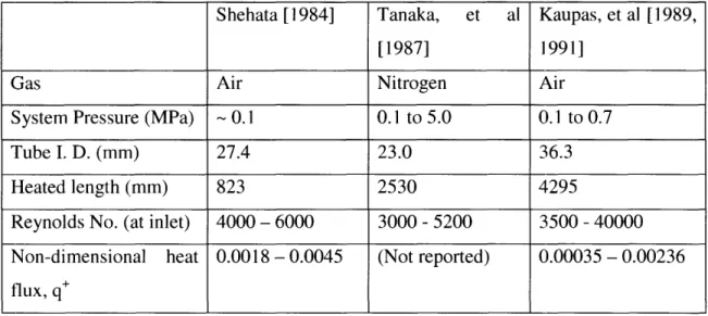
taken and where there are significant gaps in the experimental data. The following table identifies the ranges of Re number where experimental data has been taken for convection flow

regimes. From Table 2-1 it is apparent that there exists a lack of experimental data for Re <

3000. This range of Re numbers encompasses both laminar flow and the transition regime

between laminar and turbulent flows. While heat transfer correlations have been proposed for

laminar convection they still must be verified experimentally. Accurate heat transfer correlations

for the transitional regime may only be proposed after the regime has been clearly defined by experimental data.

Table 2-1 Parameters of various gas upflow experiments in heated tubes

Shehata [1984] Tanaka, et al Kaupas, et al [1989,

[1987] 1991]

Gas Air Nitrogen Air

System Pressure (MPa) - 0.1 0.1 to 5.0 0.1 to 0.7

Tube I. D. (m) 27.4 23.0 36.3

Heated length (mm) 823 2530 4295

Reynolds No. (at inlet) 4000- 6000 3000 - 5200 3500 - 40000 Non-dimensional heat 0.0018 - 0.0045 (Not reported) 0.00035 - 0.00236 flux, q

References

1. Aicher, T. and Martin, H., "New correlations for mixed turbulent natural and forced

convection heat transfer in vertical tubes," International Journal of Heat and Mass

Transfer, Vol. 40, No. 15, pp. 3617-3626, 1997.

2. Bankston, C. A., "The transition from turbulent to laminar gas flow in a heated pipe."

Journal of Heat Transfer, Vol. 92, pp. 569-579, 1970.

3. Bejan, A, Convection Heat Transfer,, Chapter 4, John Wiley & Sons, Inc., 1993.

4. Burmeister, L. C., Convective Heat Transfer, 2

_{Edition, Chapter 10 , John Wiley &}

Sons, Inc., 1993.

5. Celata, G. P., D'Annibale, F., Chiaradia, A., and Cumo, M., "Upflow turbulent mixed

convection heat transfer in vertical pipes," International Journal of Heat and Mass

Transfer, Vol. 41, pp. 4037-4054, 1998.

6. Churchill, S.W., "2.5.10 Combined free and forced convection in channels," Heat

Exchanger Design Handbook, ed. Hewitt, G.F., Begell House, Inc., 1998.

7. Jackson, J. D., Cotton, M. A., and Axcell, B. P., "Studies of mixed convection in vertical

tubes," International Journal of Heat and Fluid Flow, Vol. 10, No. 1, pp. 2-15, 1989.

8. Jackson, J. D., Personal Communication, April 1998 as referenced in Mikielewicz, D. P., et al, "Temperature, velocity and mean turbulence structure in strongly heated internal gas

flows - Comparison of numerical predictions with data," International Journal of Heat

and Mass Transfer, Vol.45, pp. 4333-4352, 2002.

9. Kaupas, V. E., Poskas, P. S., and Vilemas, J. V., "Heat Transfer to a Transition-Range Gas Flow in a Pipe at High Heat Fluxes" (2. Heat Transfer in Laminar to Turbulent Flow

Transition) and (3. Effect of Buoyancy on Local Heat Transfer in Forced Turbulent

Flow), HEAT TRANSFER-Soviet Research, Vol. 21, No. 3. pp. 340-361, 1989.

10. Tanaka, H., Maruyama, S., and Hatano, S., "Combined forced and natural convection heat

transfer for upward flow in a uniformly heated, vertical pipe," International Journal of

Heat and Mass Transfer, Vol. 30, No. 1, pp. 165-174, 1987.

11. Parlatan, Y., "Friction Factor and Nusselt Number Behavior in Turbulent Mixed

Convection in Vertical Pipes," Ph. D. Thesis, Department of Nuclear Engineering, MIT,

3. EXPERIMENTAL LOOP DESIGN

The non-dimensional parameters used to characterize convection flow regimes, Ra, Re, Bo*, and Kv will serve as guidelines for the design of the experimental thermal-hydraulic loop.

Initially the design focus will be on matching the ranges of each of the aforementioned

non-dimensional parameters encountered in post-LOCA operation of the proposed GFR. Once this

requirement is met the design focus will shift to expanding these ranges in order to provide experimental data for as many flow regimes mentioned in Table 1.1 as possible. Heat transfer in

the proposed experimental loop will be analyzed using LOCA-COLA (Loss of Coolant Accident

-- COnvection Loop Analysis), a computer code developed at MIT. LOCA-COLA was originally

developed to analyze decay heat removal by natural circulation in the GFR core. However the code is sufficiently flexible to model a variety of thermal-hydraulic loops. A detailed description of LOCA-COLA and its FORTRAN coding is given by Williams et al. [2003]

3.1 GFR LOCA-COLA Analysis

Several possible GFR block-core designs and operating conditions are described in Appendix

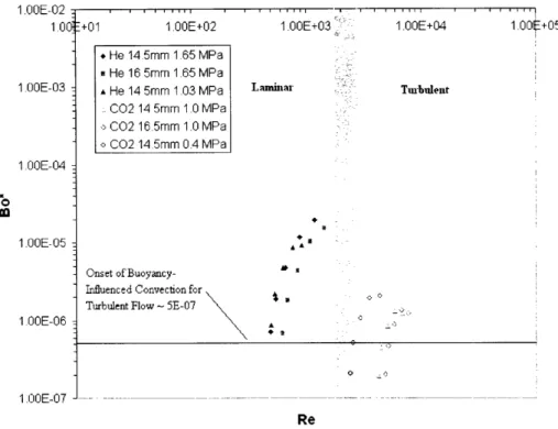
A. An analysis of the decay heat removal for these various core designs and operating conditions was conducted at MIT using LOCA-COLA. [Williams et al. 2003] Figures 3-1, 3-2, and 3-3 are

graphs of the four relevant non-dimensional parameters for convection, Ra, Re, Bo*, and Kv,

measured along a core channel from inlet to outlet for the various geometries and operating conditions of the GFR. As expected, the GFR operates predominantly in a mixed convection regime following a LOCA (Figure 3-1). Perhaps more importantly, Figure 3-1 also shows that

the GFR will operate in the transition regime between laminar and turbulent mixed convection

and mixed and forced convection. As mentioned in the previous chapter, the transition between

forced and mixed convection is characterized by the onset of buoyancy-aided convection. Figure

3-2 is evidence of this fact as it shows that a significant portion of the turbulent flow encountered in the GFR loop will experience the onset of buoyancy-influenced convection. As a result it is important for the experimental loop to be able to generate data both above and below the onset of

of the GFR loop will not exhibit lower heat transfer characteristics due to laminarization of the

flow. As a result operation of turbulent flow regimes where laminarization is prominent should

be avoided in the experimental loop in order to reproduce the heat transfer characteristics of the

GFR loop. Turbulellnt Forced .-Convection Transitional A A A A I A Laminar A_.9- * 6 f IL As -?Mixed

C'onvection,_{- Tbble enttT}

X /

~~~Free

1.00E+01 1.OOE+02 1.00E+03 1.00E+04 1.00OE+05 1 OOE+06 1.00E+07 1.00E+08 1.00E+09

Ra

Figure 3-1 Ra vs. Re map for reactor prototype loop

I .UUE'tUCU 1 .00E+05I 1 00E+04 I 1 00E+03 1 OOE+02 1 OOE+01 1 OOE+OCI " mE- , : -.... " . . . , ... I . , . . - - . .

1.OOE-02: 1.0 1.00E-03 1.OOE-04 to 1.OOE-05 1.OOE-06 --.f7 --+01 1.OOE+02 Onset of Buoyancy-Ifluenced Convection for

Turbulent Flow - 5E-07

1.00E+03 Lamhlar

~~~:

a

Figure 3-2 Buoyancy parameter for reactor prototype loop

3:

.00.

4

15

6

-+01 1 .OOE+02 1 .OOE+0... OOE+O3 ?t

r- : L asinkar 1.OOE+04 Turbldlent * * Ag * , A A . Laminarization of Turbulent Flow Prominent - 4E-06 0oo -0 0 0 &%7'? _C, Re

Figure 3-3 Acceleration parameter for reactor prototype loop

* He 14.5mm 1.65 MPa * He 16 5mm 1.65 MPa A He 14 5mm 1.03 MPa C02 14 5mm 1.0 MPa , C2 16.5mm 10 MPa o CO2 14.5mm 0.4 MPa 1.OOE + He 14.5mm 1.65 MPa · He 16.5mm 1.65 MPa A He 14.5mm 1.03 MPa _ C02 14.5mm 1.0 MPa o, C02 16.5mm 1.0 MPa o C02 14.5mm 0.4 MPa 1 .00E+05 1 00E-0 1.( 1 .00E-0' 1 .00E-0 1 OOE-0( 1.OOE-0O 1 S - - - . = - s -f~ , , ., .,, , * , ., . .. . . 1 1.00,05 i i

t .

3.2 Experimental Loop Design

As mentioned previously, the experimental loop was designed with two objectives in mind,

the first being to encompass the entire range of post-LOCA operating conditions as depicted in

Figures 3-1, 3-2, and 3-3, while the second being to encompass as many of the flow regimes portrayed in Table 1 .1l as possible. In addition to filling in experimental gaps in convection flow regimes the second objective will allow the heat transfer analysis to be extended into flow regimes where heat transfer correlations are well established, i.e. turbulent and laminar forced convection. As a result, we will be able to benchmark some of our data and resulting heat transfer correlations with those found in the literature.

3.2.1 Design Considerations and Constraints

We were initially faced with several considerations when contemplating the design for the experimental loop. First we wanted to keep a certain degree of similitude between the geometry of the GFR (prototype) loop and the experimental loop, as key non-dimensional parameters such as Ra and Re number are dependent upon the hydraulic diameter (inner diameter of the tube). As a result a test section diameter of 16mm and length of 2m was chosen to closely match the

prototype loop (For GFR geometry see Appendix A). Secondly, since most of the experimental runs may utilize natural circulation, we wanted to maximize the available driving force from this source. To this end, the thermal elevation difference between the heated channel and the heat exchanger was set at a maximum value of 4.25m (limited by the height of the lab space available).

Another main design consideration for the loop resulted from the addition of a hot-wire probe for measuring local fluid velocity and temperature profiles in the heated test section. Accurate calibration of this hot-wire probe above 450°C is extremely difficult. As a result the maximum bulk fluid temperature for the heated test section will be restricted to 450°C. This constraint is actually very significant as the coolant flow in the GFR prototype is greater than

1000°C for some cases. And since non-dimensional scaling parameters for convection flow regimes are dependent upon temperature, we will have to compensate for the reduced operating

temperature of the experimental loop. The presence of the probe also leads to one more design modification. An extra heated test section with a diameter of 32mm was incorporated into the

loop design, as a larger test section diameter will result in more accurate probe data. However

this extra test section, with a hydraulic diameter twice that of the original test section, will also

serve to increase the range of non-dimensional parameters encompassed by the experimental

loop. The two heated test sections will be interchanged depending upon whether accurate

prototype representation or probe data is desired.

One more constraint for the bulk fluid temperature arises from the fact that the experimental loop will incorporate a blower in order to reach forced convection regimes. The blower will be

located in the cold leg of the experimental loop and will limit the maximum temperature of the

fluid in the cold leg to I 00°C as the rubber gaskets of the blower cannot exceed that temperature.

Finally, the wall temperature in the heated test section is limited to 650°C to meet ASME code

requirements at the maximum system pressure of 1.0 MPa for stainless steel 316.

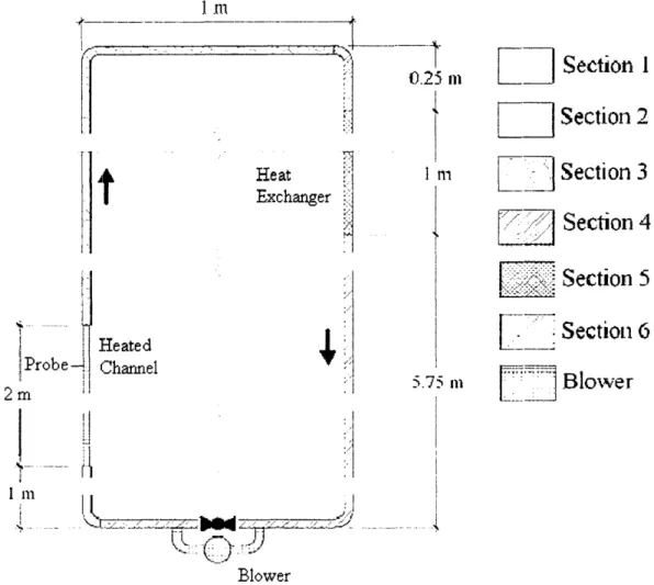
3.2.2 Loop Description

Based upon the aforementioned design considerations, we arrived at the experimental loop

depicted in Figure 3-4. The relevant component dimensions and descriptions are listed in Table 3.1. The overall dimensions of the loop are 7m high by m wide with 25.4mm ID tubing, the thermal elevation difference is 4.25m, the heated section of the loop is 2m long with either an ID of 16 or 32mm, and the heat exchanger has a length of 2m and a height of lm. The heat

exchanger length of 2 meters was calculated based upon counter flow with a constant wall

temperature of 27°C. Stainless Steel 316 was the material of choice for the loop as it is relatively

inexpensive and met ASME requirements at maximum system pressure and temperature.

L

Section

2m!

Lii

EIi:

. Section

6

:

t

lower

II

I

-

__

I__

--1

1

l

Figure 3-4 Experimental loop diagram

Table 3-1 Component description of experimental loop

Section

Description

Diameter

Material

AZ

Length

1 Upcomer 25.4 mm SS 316 1.00 m 1.00 m

2 Heated CH. 16,32 mm SS 316 2.00 m 2.00 m

3

HotLeg

25.4 mm

SS 316

4.00 m

5.00 m

4 Downcomer 25.4 mm SS 316 0.25 m 0.25 m

5 Heat Ex. Tube in Tube Cu 1.00 m 2.00 m

6 Cold Leg 25.4 mm ISS 316 5.75 m 6.75 m

1 m1 i

Section 2

Section 3

Section 4

3.3 LOCA-COLA Analysis of Proposed Experimental Loop

Having established the key dimensions of the experimental loop for input into

LOCA-COLA, the next step is to determine the maximum range of non-dimensional convection

parameters the loop can generate. This will be accomplished by running LOCA-COLA

simulations utilizing both the 6mm and 32mm diameter test sections along with three gases, helium, nitrogen, and carbon dioxide, with pressures ranging from 0.1 MPa to 1.0 MPa.

3.3.1 Helium Trial Calculations

Six trials were conducted using helium as the test fluid with the variables being test section diameter and system pressure. For each trial the heat flux was adjusted to approach the

maximum fluid bulk temperature of -450 °C. Also for every trial the heat exchanger had a

constant wall temperature of 27°C. Table 3.2 contains the three main inputs for the trials; test

section diameter, system pressure, and heat flux, along with the resulting output loop parameters

for each trial.

Table 3-2 LOCACOLA inputs and resulting parameters for He coolant

Heat Twall Flow Pressure Total

ID Pressure Flux Tin Tout Max Rate Drop Heat Velocity* Re*

mm MPa kW/m^2 C C C kg/s Pa kW mrn/s 16.0 0.2 0.50 27 456 457 2.25E-05 9.16 0.050 0.49 63 16.0 0.6 4.00 29 443 490 1.87E-04 25.90 0.402 1.37 529 16.0 1.0 8.00 47 411 512 4.25E-04 36.30 0.804 1.92 1210 32.0 0.2 0.45 27 435 441 4.27E-05 8.99 0.091 0.23 61 32.0 0.6 3.00 40 411 476 3.14E-04 22.20 0.603 0.58 449 32.0 1.0 5.50 73 409 521 6.34E-04 30.50 1.110 0.75 887

*Denotes average value in heated section

3.3.1.1 Scaling Ra number

As stated previously the main concern in scaling the Ra numbers between the prototype and model is the fact that the much higher temperatures of the prototype allow for a lower range of Gr numbers which in turn leads to lower Ra numbers. However looking at Figure 3-5 we see that

with helium the model

loop

101

which completely encompasses the range of Ra numbers found for the prototype. If we look a

little closer at Figure 3-5 we see that the two trials conducted at 0.2 MPa generate the lowest ranges of Ra numbers. Now besides the fact that these two trials were conducted at the same

system pressure they have one other important similarity, a very small temperature difference

between the maximum wall temperature and bulk fluid exit temperature. For the 16 mm test section at 0.2 MPa this difference is only °C, and for the 32 mm test section at 0.2 MPa this

difference is only 6 C. (For helium in the prototype this difference is 100 C) This latter

similarity is the reason why the 0.2 MPa cases can generate lower Ra number ranges as the Gr number is proportional to the difference between the temperature of the wall and the bulk fluid temperature, (Tw-Tb). 1.OOE+06 1.00E+05 1.00E+04 1.00E+03 1.OOE+02 1.00E+01 1.00E+00 Tiubldent .. . .. Forced C ontvection . - Tmbldent lxed - C

~Colnvectiolt

.

~*

^

[*

*

He16mm0.6MPa

1.00E+01 1.00E+02 1.00E+03 1.00E+04 1.00E+05 1.00E+06 1.00E+07 1.00E+08 1.00E+09

Ra

Figure 3-5 Ra vs. Re map for experimental loop with He coolant

3.3.1.2 Scaling Bo* number

The Buoyancy parameter is important for its influence upon convection. According to Jackson [1989], buoyancy-influenced turbulent convection in round tubes occurs when Bo* - 5 x 10- 7. This is important as the prototype Bo* number range of 2 x 10-7 to 3 x 10-5includes this value for the onset of buoyancy-influenced turbulent convection. However, looking at Figure 3-6, we see that buoyancy-influenced turbulent convection is irrelevant in the helium trial calculations as the flow is laminar for every case. As a result, we will look to nitrogen and carbon dioxide to generate turbulent flows, where buoyancy-influenced convection is relevant.

1 .00E+02 0 [I c 1 .00E+03 Lmnhtar } z= Lamular~~~~~~~~~~- : z. . . . U3 U 11 0 0 I_0 & t A Onset of Buoyancy- · :

Influenced Convection for

Turbulent Flow 5E-07 I

Re

Figure 3-6 Buoyancy parameter for experimental loop with helium coolant

E+01 1 .00E+04 1.00E+05

1.OOE02 -1.0([ 1.OOE-03 1.OOE-04 o0_Do 1.OOE-05 1.OOE-06 1.OOE-07 * 16mm 0.2 MPa i 16mm 0.6 MPa , 16mm 1.0 MPa [ 32mm 0.2 MPa 32mm 0 6 MPa o 32mm 1.0 MPa Tiubldent -1 S

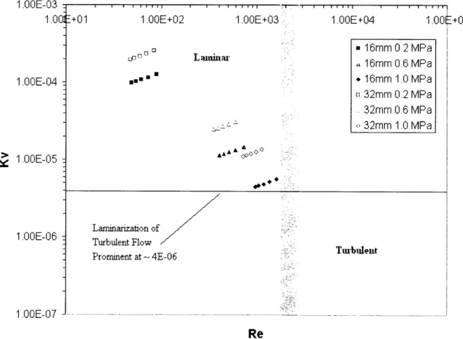
3.3.1.3 Scaling Kv parameter

As stated in Chapter 2, the acceleration parameter is important in determining if

laminarization is likely to occur in turbulent flow. As per McEligot and Jackson [2004], laminarization is prominent at Kv 4 x 10-6. On the other hand, laminarization is unimportant when Kv < I x 10-6. However, as stated previously, all of the helium trial calculations resulted in laminar flow where the process of laminarization is not relevant. As a result the acceleration

parameter is simply representative of the acceleration of the gas flow and is plotted here for

completeness. Figure 3-7 shows that helium will operate in a Kv range of 4 x 10-6_{to 3 x 10}-4 .

-+01 1 .00E+02 Fran LPm-ME U I . , , I , I A, 1 .00E+03 Lamina' 1.OOE+04 1.00t+05 ,AA & 0 _:~'0 Lanminarization of Turbulent Flow Prominent at - 4E-06 i'. ; ' :=::

. =~~~ublet

Figure 3-7 Acceleration parameter for experimental loop with helium coolant

-1 anCd) r I .UUL---UO -1.00 1.00E-04 i 1.00E-05 1 .00E-06 I nn n7 * 16mm 0.2 MPa ,, 16mm 0.6 MPa * 16mm 1.0 MPa n 32mm 0.2 MPa 32mm 0.6 MPa < 32mm 1.0 MPa Ii . . . -- l l l | l l l l l l i l i ,.wu - I .. l _ _ _ _ _ _ _ _ _ _ _ _

3.3.2 Nitrogen Trial Calculations

The experimental setup for nitrogen is very similar to that of helium, namely the same input

parameters and constraints were considered. However, since the area of overlap between the

relevant non-dimensional parameters of the two coolants occurs at higher helium pressures and

lower nitrogen pressures, the system pressure for the nitrogen coolant was extended down to 0.1

MPa for both the 16 and 32 mm test sections to create a larger overlap. As a result we will be

able to compare heat transfer correlations developed from the two coolants for a larger flow

regime area. However it should be noted that for 5 out of the total 8 trials the inlet temperature of

the test section is greater than 100°C, which violates the maximum temperature for the rubber

gaskets of the blower. This problem is easily solved as the inlet temperatures of the test section

can be brought below 100°C by simply increasing the length of the heat exchanger.

Table 3-3 LOCACOLA inputs and resulting parameters for N2 coolant

Heat Twall Flow Pressure Total

ID Pressure Flux Tin Tout Max Rate Drop Heat Velocity* Re*

Mm MPa kW/m^2 C C C kg/s Pa kW mrn/s 16.0 0.1 1.10 37 446 521 2.54E-04 28.70 0.111 1.62 773 16.0 0.2 2.50 79 435 611 6.62E-04 43.30 0.251 2.29 1970 16.0 0.6 5.50 130 428 565 1.73E-03 94.00 0.553 2.18 4980 16.0 1.0 8.00 157 435 557 2.69E-03 134.00 0.804 2.13 7560 32.0 0.1 0.80 58 440 534 3.96E-04 24.80 0.161 0.66 595 32.0 0.2 1.50 113 414 572 9.40E-04 33.80 0.302 0.86 1380 32.0 0.6 3.00 161 406 620 2.30E-03 73.10 0.603 0.75 3280 32.0 1.0 4.55 174 398 661 3.81E-03 108.00 0.915 0.76 5410

*Denotes average value in heated section

3.3.2.1 Scaling Ra number

lit

is apparent from Figure 3-8 that the model utilizing nitrogen cannot cover the lower portion of

the prototype Ra number range. However nitrogen does provide an overlap of Ra numbers

between itself and helium from I x 103 to I x 106, which will prove useful for future

comparisons. Furthermore the use of nitrogen as a coolant allows us to extend the operating

range of the loop further into turbulent mixed convection and even across the boundary between

mixed and free convection. This is important as data taken from the transition region between

mixed and free convection may be used to verify the boundary between mixed and free

convection proposed by Burmeister [1993].

1 .00E+06 1.00E+05 1.00E+04 4) 1OE0 1.00E+02 1.00E+01 1.OOE+00 -Turbullent Forced

Conv ectionl _{. Tubulent}

Mix led Convection' AAAAAA A t A As A, A & , &AA f : Tranlsitiondal -A -A -A T IUL' _

1.00E+'01 1.00E+02 1.00E+03 1.00E+04 1.00E+05 1.00E+06 1.00E+07 1.00E+08 1.00E+09

Ra

Figure 3-8 Ra vs. Re map for experimental loop with nitrogen coolant

3.3.2.2 Scaling Bo* number

As mentioned in section 3.3.1.2 an important Bo* number is approximately 5 x 10-7as it signals

the onset of buoyancy-influenced convection in turbulent flow. Also, as mentioned previously

the model loop utilizing helium was unable to generate Bo* numbers this low. However, when the coolant in question is nitrogen the Bo* number range is approximately 4 x 10-7to 4 x 10-4, as shown in Figure 3-9. As a result we should be able to observe the onset of buoyancy-influenced convection for turbulent flow in the model loop (boundary between forced and mixed

convection).

-+01 1 .OOE+02

Onset of Buoyancy-Influenced Convection for Turbulent Flow -5E-07

, , , , , . i . ., . 1 .OOE+03=; -_ Lmaninlari :' X X

x0!

Figure 3-9 Buoyancy parameter for experimental loop with nitrogen coolant

3.3.2.3 Scaling Kv number

From Figure 3-10 we see that the model loop utilizing a nitrogen coolant is able to extend the Kv range covered by helium down to approximately 5 x 10- 7. As a result, the range of Kv

numbers encompassed by the loop utilizing nitrogen as a coolant completely encompasses the

transition region from where laminarization goes from being unimportant to being prominent, 5 x 1 0- 7 to 4 x 10-6. However, as was mentioned previously, the process of laminarization is only important when the flow is turbulent, i.e., the Re number is greater than 2300. But while the Kv values above the threshold value of 4 x 10-6 occur for laminar flow they are sufficiently close to

the transitional region between laminar and turbulent flow to merit close attention.

1 00+05 * 16mm 0.1 MPa * 16mm 0.2 MPa , 16mm 0.6 MPa a 16mm 1.0 MPa x 32mm 0.1 MPa o 32mm 0.2 MPa 32mm 0.6 MPa . 32mm 1.0 MPa 1.OO0E-02 1.00 1 .OOE-03 1.OOE-04 ,K C Om 1.OOE-05 1.OOE-06 1.00E-07 1 .OOE+04 Tiubident o o _a O C, a A A A -_ An A_ai - - - = ... . . . . ,,,,, . , ,,,,,, f , * , ,,,,,

1 .00E-03 1.0c 1.00E-04 > 1.00E-05 1 .00E-06 1 .00E-07 -+01 1.00E Laminarization of Turbulent Flow -Prominent - 4E-06 I I . ... I' 7., -+02 1.00E+'03

Laminar

=;

\~~~~~*

*f *

t

Re

Figure 3-10 Acceleration parameter for experimental loop with nitrogen coolant

3.3.3 Carbon Dioxide Trial Calculations

The carbon dioxide trials, like the nitrogen trials, utilized a lower system pressure, 0.1 MPa,

to provide for a larger area of overlap between the coolants. However, in this case lowering the

pressure turns out to be even more effective as we can now compare heat transfer correlations

developed from three different coolants for the same flow regimes.

1 .00E+04 1 ₀ L 0 5 1 .001 ~+05 * 16mm 0.1 MPa . 16mm 0.2 MPa A 16mm 0.6 MPa a, 16mm 1.0 MPa x 32mm 0.1 MPa o 32mm 0.2 MPa 32mm 0.6 MPa o 32mm 1.0 MPa ,,., - - , .~~~~~~~~~~~- .

I

t0aa

A

OP~~~~Tlbln

Table 3-4 LOCACOLA inputs and resulting parameters for C02 coolant

Heat Twall Flow Pressure Total

ID Pressure Flux Tin Tout Max Rate Drop Heat Velocity* Re* Mm MPa kW/m^2 C C C kg/s Pa kW mrn/s 16.0 0.1 2.10 68 485 623 4.88E-04 39.30 0.211 2.15 1500 16.0 0.2 3.25 103 419 632 1.00E-03 58.00 0.327 2.28 3160 16.0 0.6 7.00 151 409 517 2.60E-03 127.00 0.704 2.12 7960 16.0 1.0 10.00 177 406 511 4.14E-03 178.00 1.005 2.09 12500 32.0 0.1 1.20 101 423 557 7.25E-04 29.50 0.241 0.83 1140 32.0 0.2 2.00 140 418 601 1.38E-03 45.80 0.402 0.84 2120 32.0 0.6 4.20 177 397 647 3.63E-03 102.00 0.845 0.76 5490 32.0 1.0 7.80 166 387 627 6.74E-03 180.00 1.568 0.83 10400

*Denotes average value in heated section

3.3.3.1 Scaling Ra number

Carbon dioxide as a coolant in the model loop serves a similar function as the nitrogen coolant. Namely it allows us to compare results between more than one coolant for the same Ra number and it also allows us to extend the range of Ra numbers encompassed by the model loop. (Figure 3-1 1) More specifically we will be able to compare results from all three coolant fluids fior a Ra number range of approximately I x 104 to x 106, and a Re number range of roughly 1000-2000. The carbon dioxide trials also allow us to obtain more data for the transition from

Ttu'bildent Forced Convection Trasitional Lanilnar -i i Tubildent Mfixed Convection, milent Lee i ectionl CO2 1e C02 32 C2 32 C02 32 o C02 3 D Pa IP~ i~ 6mm 1.0 MPa ,mm 0.1 MPa 'mm 0.2 MPa 2mm 0.6 MPa _mm 1.0 MPa

1.00E+01 1.00E+02 1.00E+03 1.00E+04 1.00E+05 1.00E+06 1.00E+07 1.00E+08 1.00E+09

Ra

Figure 3-1 1 Ra vs. Re map for experimental loop with carbon dioxide coolant

3.3.3.2 Scaling Bo* number

Since we have already established the fact that we can encompass the regime of buoyancy-influenced convection, the only objective left is to extend the model loop Bo* to lower values in order to encompass more of the prototype Bo* range of 2 x 10- 7to 3 x 10-5, i.e., dominant forced

convection. Figure 3-12 shows that the lowest possible Bo* number obtained in the model loop

utilizing the carbon dioxide coolant is approximately 2.5 x 10-7, and while the prototype Bo* range extends to a slightly lower value, the difference is negligible.

4 nIl' n-I -U -- TU .I 1.OOE+05 1.OOE+04 g 1.00E+03 1 .00E+02 1.OOE+01 I .UUt+UU I 1 l1 lU+l In A-,aA Z A, I A A AAA I A' I I . , , - ,

.,

,

.

.I

.-..

+131 1.OOE+02 , , ,,,, ,i .= 1 .00E+03 ' Lainirnar x 'C 0 x O x 0 ru Onset of Buoyancy-Influenced Convection for

Turbulent Flow 5E-07 I

. .

-- ff

Re

Figure 3-12 Buoyancy parameter for experimental loop with carbon dioxide coolant

3.3.3.3 Scaling Kv number

The carbon dioxide trials pose the most difficulty in avoiding laminarization of turbulent

flow in the mixed convection regimes. Looking at Figure 3-13 we see that the trial runs

operating in the transition region between laminar and turbulent flow have Kv values greater than

4 x 10-6. Whether laminarization in this transition region is important or not will have to be

determined experimentally.

:

1 .00E03 -1.00i 1.00E-04 :" 1.00E-05 1 .OOE-06 1 nnfP n7 Z+01 1 .00E+02 Lain Laminanization of Turbulent Flow Prominent - 4E-06 Re

Figure 3-13 Acceleration parameter for experimental loop with carbon dioxide coolant

3.3.4 Trials Utilizing the Blower

While we were able to completely map the mixed convection region of the GFR conditions

using our various input parameters under the guiding force of natural circulation, we would like

to be able to generate data from both laminar and turbulent forced convection regimes in order to

compare with accepted heat transfer correlations and analyses for the aforementioned regimes.

Furthermore we will only utilize helium for these trials as the nitrogen and carbon dioxide

coolants would require much more heat input to reach turbulent-forced convection. As the onset

of turbulent flow occurs at a Re number of approximately 2300, we will need to generate data

both significantly below and above this number for comparison to accepted results. Figure 3-14

is a Ra vs. Re map for helium coolant utilizing the blower. From the figure we can see that at a pressure of 0.1MPa with 1.1 KW deposited in the flow we can generate a laminar forced convection regime with a Re number range of approximately 1000-1900. And as we increase the

1.OOE+03 />: LI~~~~~~~~~kr~/-5 := = 1191'~~~~~~~~~~~t: 1.OOE+04 Tmbit 0.1 MPa 0.2 MPa 0.6 MPa 1.0 MPa 0.1 MPa 0.2 MPa 0.6 MPa 1.0 MPa I i i i i 1 7 1.001--+05 Ldent x x xx X x x .j _ =C *-1 l * , & ..., , ,, i,, l * 16MM m 16mm A 16MM A 16MM x 32mm o 32mm ; 32mm o 32mm am- i i i I I i IL 4A _i i i InO04A i

__

__

pressure and power we can generate a turbulent forced convection regime with a Re number

range of approximately 4000-10000.

ANAsiAS* ,.--.' .AConvection/ Tmbldlent

Fiee Transitionll~ _{* A- = * na1 U} : -=:~/Fe _Convection

* He 6mm O.1MPa 1.1 KW

Laminiar Ai He 16mm -1MPa 15 KW

* He 16mm 0.2MPa 3.0 KW

He 16mm 0.6MPa 2.5 KW

1.OOE+01 1.OOE+02 1.OOE+03 1.OOE+04 1.OOE+05 1.OOE+06 1.OOE+07 1.OOE+08 1.OOE+09

Ra

Figure 3-14 Turbulent and laminar forced convection for experimental loop with He coolant

3.4 LOCA-COLA Analysis Summary

In the preceding sections it has been shown that through the use of three fluids, helium, nitrogen, and carbon dioxide, two test section diameters, 16 and 32 mm, and varying system pressures, 0.1 MPa- 1.0 MPa, that the relevant dimensionless parameters, Ra, Re, K , and Bo* can be conserved from the GFR prototype to the experimental model. Figures 15, 16, and 3-17 are graphs of the entire ranges of the Ra, Re, Kv, and Bo* numbers resulting from natural

circulation for both the prototype and model. Furthermore in addition to covering the entire

range of reactor conditions our second objective was to encompass as many of the nine flow and

heat transfer regimes mentioned in Table 1.1 From Figure 3-15 it is apparent that we can cover laminar, transitional, and turbulent mixed convection flows. And since we can also control the

I 111 lRtl or]

-4) X

Re number through use of the blower we should be able to operate in mixed and forced

convection for laminar, transitional, and turbulent flows. Figures 3-16 and 3-17 act, respectively,

as guidelines to determine whether buoyancy-influenced convection and/or laminarization effects

are likely to be important. As a result using the experimental loop we should be able to develop heat transfer correlations that are not only applicable to the GFR prototype loop but to a larger range of flow and convection regimes.

,4 er t-. ehae

Tiubldent .

Forced

Convection

_{I tmblent}

lixed Convection./ LAA t O11

-

:

Tranisitional

+ ,* t S

1.OOE+O01 1.OOE+02 1.OOE+03 1.OOE+04 1.OOE+05 1.OOE+06 1.OOE+07 1OE+08 1OE+09

Ra

Figure 3-15 Complete Ra vs. Re map generated from experimental loop

I .uut-+Uo 1.OOE+05 1.OOE+04

.4).E+03

---

1 .0OE+02 Laminar ,,, 1.OOE+03 1 .OOE+O3 - 1 .0OE+04 * Prototype - A Model - Helium * Model- Nitrogen

* Model- Carbon Dioxide

Turbulent

N . XB

!,

A. ·

Onset of Buoyancy-Influenced Convection for Turbulent Flow- 5E-07

I *. , 4, *-* : A * * d *- . U . . * Ua A 3 I I 4® W · A 9, \ _{* A}* _ _ 9· 9 - O I W# U1 U 9 a - tk . - 9* , 14. Re

Figure 3-16 Range of Buoyancy parameter generated from experimental loop

4 nnor nl' I UUE_-UC 1.i 1.OOE-O 1. 00E-O 1 .OOE-O I nnr n-+05 Re

Figure 3-17 Range of acceleration parameter generated from experimental loop

:+01 'i .Ov~ v 1 .00E-03 1.OOE-04 # m 1.00OE-05 1.00OE-06O 1 nnF-07

-" -"I;

I

.;:

-References

1. Burmeister, L. C., Convective Heat Transfer, 2

Edition, Chapter 10, John Wiley &

Sons, Inc., 1993.

2. Jackson, J. D., Cotton, M. A., and Axcell, B. P., "Studies of mixed convection in vertical tubes," International Journal of Heat and Fluid Flow, Vol. 10, No. 1, pp. 2-15, 1989.

3. McEligot D.M. and Jackson J.D., "Deterioration Criteria for Convective Heat

Transfer in Gas Flow Through Non Circular Ducts," INEEL/JOU-03-01311, INEEL

Report, Revised 2004. Also published in Nuclear Engineering and Design, 2004.

4. Williams W. C., Hejzlar P., Driscoll M. J., Lee W. J., and Saha P., "Analysis of a

Convection Loop for GFR Post-LOCA Decay-Heat Removal from a Block- Type

Core," Topical Report MIT-ANP-TR-095, Massachusetts Institute of Technology,

Department of Nuclear Engineering, 2003.

4. LOOP CONSTRUCTION

Having verified that the proposed experimental loop design can operate in the flow regimes

of interest, the next stage in the project was construction of the loop. Actual fabrication of the

experimental loop was broken down into three stages. In the first stage the components of the loop, as described in Table 3-1, along with the power supply and forced convection system are

assembled. In the second stage the instrumentation necessary for acquiring experimental data for

use in calculating heat transfer coefficients and non-dimensional parameters is installed in the

loop. Finally in the last stage insulation and guard heaters are applied to the test section and hot leg of the loop to reduce heat loss to the environment and maintain bulk fluid temperature.

4.1 Main Components

The entire loop is composed of Stainless Steel 316 tubing with an inner diameter of 25.4 rmm, with the exception of the test section, which either has an inner diameter of 16 or 32 mm.

The various sections of the loop are connected with stainless steel compression fittings. The test

section is connected to the rest of the loop by reducing unions. Furthermore this transition has been made as smooth as possible as a taper has been inserted just upstream of the test section to ensure minimum disturbance while the fluid flow is developing.

A counter flow tube in tube heat exchanger was selected for the loop as it best met the heat

transfer requirements of the loop. The heat exchanger itself is composed of 6 loops with an

average diameter of 30.5cm (12 in) for an overall length of approximately 5.75m. However the

heat exchanger from the top to bottom coil is only roughly 0.5m, half the height of the heat

exchanger used in the LOCA-COLA analysis, which as a result actually provides a slight increase

in the available driving head for natural circulation. Furthermore since the heat exchanger length assumed in the LOCA-COLA analysis was 2m the actual length of 5.75m will be more than sufficient to cool bulk fluid temperatures below 100°C. Also over-cooling of the fluid will not be an issue since the flow rate of the cooling water into the heat exchanger can be adjusted.

The test section will be resistively heated utilizing a 1500-ampere DC power supply. The

power supply is connected to the exterior wall of the test section by a copper clamp at the bottom

section. The level of heat input to the test section will be correlated with the electrical current

provided by the power supply.

While the majority of the experimental trials will be conducted utilizing natural circulation,

forced convection regimes can only be reached in the experiment with the addition of an external

driving force. A forced convection system consisting of a compressor connected to an

accumulator tank provides this driving force. Fluid flow is first branched off of the bottom

horizontal section of the loop and taken to the compressor. The flow is then directed into the accumulator tank, where the compressed flow is smoothed before re-entering the main loop. From there the flow is reintroduced into the main loop through another valve located in the bottom section of the loop.

4.2 Instrumentation

In order to calculate heat transfer coefficients knowledge of the wall temperatures, heat

deposited in the fluid, fluid velocities, and pressure drops in the system is required. As a result extensive instrumentation for the experimental loop is required. Figure 4-1 is a complete Process and Instrumentation Diagram for the experimental loop. The rest of this section is a detailed description of the instrumentation beginning with the test section and moving in the direction of the flow as depicted in Figure 4-1.