HAL Id: hal-01492982
https://hal.sorbonne-universite.fr/hal-01492982
Preprint submitted on 20 Mar 2017HAL is a multi-disciplinary open access
archive for the deposit and dissemination of sci-entific research documents, whether they are pub-lished or not. The documents may come from teaching and research institutions in France or abroad, or from public or private research centers.
L’archive ouverte pluridisciplinaire HAL, est destinée au dépôt et à la diffusion de documents scientifiques de niveau recherche, publiés ou non, émanant des établissements d’enseignement et de recherche français ou étrangers, des laboratoires publics ou privés.
Resistance metric, and spectral asymptotics, on the
graph of the Weierstrass function
Claire David
To cite this version:
Claire David. Resistance metric, and spectral asymptotics, on the graph of the Weierstrass function. 2017. �hal-01492982�
Resistance metric, and spectral asymptotics, on the graph
of the Weierstrass function
Claire David
March 20, 2017Sorbonne Universités, UPMC Univ Paris 06
CNRS, UMR 7598, Laboratoire Jacques-Louis Lions, 4, place Jussieu 75005, Paris, France
1
Introduction
Following our work on the graph of the Weierstrass function [Dav17], in the spirit of those of J. Kigami [Kig89], [Kig93], and [Str99], [Str06], which enabled us to build a Laplacian on the aforementioned graph, it was natural to go further and give the related explicit resistance metric.
The aim of this work is twofold. We had a special interest in the study of the spectral properties of the Laplacian. In [Dav17], we have given the explicit the spectrum on the graph of the Weierstrass function. In the case of Laplacians on post-critically finite fractals, previous works, by J. Kigami and M. Lapidus [KL03], and R. S. Strichartz [Str06], make the link between resistance metric, and asymp-totic properties of the spectrum of the Laplacian, by means of an analoguous of Weyl’s formula.
So we asked ourselves wether those results were still valid, for the graph of the Weierstrass function.
2
Framework of the study
In this section, we recall results that are developed in [Dav17].
Notation. In the following, λ and Nb are two real numbers such that:
0 < λ < 1 , Nb ∈ N and λ Nb > 1
We will consider the (1−periodic) Weierstrass function W, defined, for any real number x, by: W(x) =
+∞
∑
n=0
λn cos (2 π Nbnx)
We place ourselves, in the sequel, in the Euclidean plane of dimension 2, referred to a direct or-thonormal frame. The usual Cartesian coordinates are (x, y).
The restriction ΓW to [0, 1[×R, of the graph of the Weierstrass function, is approximated by means of a sequence of graphs, built through an iterative process. To this purpose, we introduce the iterated
function system of the family of C∞ contractions fromR2 toR2: {T0, ..., TNb−1}
where, for any integer i belonging to{0, ..., Nb− 1}, and any (x, y) of R2:
Ti(x, y) = ( x + i Nb , λ y + cos ( 2 π ( x + i Nb ))) Property 2.1. ΓW = N∪b−1 i=0 Ti(ΓW)
Definition 2.1. For any integer i belonging to{0, ..., Nb− 1}, let us denote by:
Pi= (xi, yi) = ( i Nb− 1 , 1 1− λ cos ( 2 π i Nb− 1 ))
the fixed point of the contraction Ti.
We will denote by V0 the ordered set (according to increasing abscissa), of the points:
{P0, ..., PNb−1}
The set of points V0, where, for any i of{0, ..., Nb− 2}, the point Pi is linked to the point Pi+1,
con-stitutes an oriented graph (according to increasing abscissa)), that we will denote by ΓW0. V0 is called
the set of vertices of the graph ΓW0.
For any natural integer m, we set:
Vm= N∪b−1
i=0
Ti(Vm−1)
The set of points Vm, where two consecutive points are linked, is an oriented graph (according to
increasing abscissa), which we will denote by ΓWm. Vm is called the set of vertices of the graph ΓWm.
We will denote, in the sequel, by
NmS = 2 Nbm+ Nb− 2
the number of vertices of the graph ΓWm, and we will write:
Vm=
{ Sm
0 ,S1m, . . . ,SNmm−1
Figure 1: The polygonsP1,0,P1,1,P1,2, in the case where λ =
1
2, and Nb= 3.
Figure 2: The graphs ΓW0 (in green), ΓW1 (in red), ΓW2 (in orange), ΓW (in cyan), in the case where λ = 1
2, and Nb= 3.
Definition 2.2. Consecutive vertices on the graph ΓW
Two points X et Y de ΓW will be called consecutive vertices of the graph ΓW if there exists a natural integer m, and an integer j of{0, ..., Nb− 2}, such that:
X = (Ti1◦ . . . ◦ Tim) (Pj) et Y = (Ti1 ◦ . . . ◦ Tim) (Pj+1) {i1, . . . , im} ∈ {0, ..., Nb− 1}
or:
X = (Ti1 ◦ Ti2 ◦ . . . ◦ Tim) (PNb−1) et Y = (Ti1+1◦ Ti2. . .◦ Tim) (P0)
Definition 2.3. For any natural integer m, the NmS consecutive vertices of the graph ΓWm are, also,
the vertices of Nbm simple polygons Pm,j, 06 j 6 Nbm− 1, with Nb sides. For any integer j such
that 06 j 6 Nbm− 1, one obtains each polygon by linking the point number j to the point num-ber j + 1 if j = i mod Nb, 06 i 6 Nb− 2, and the point number j to the point number j − Nb+ 1
if j =−1 mod Nb. These polygons generate a Borel set ofR2.
Definition 2.4. Polygonal domain delimited by the graph ΓWm, m ∈ N
For any natural integer m, well call polygonal domain delimited by the graph ΓWm, and denote
byD (ΓWm), the reunion of the N
m
b polygons Pm,j, 06 j 6 Nbm− 1, with Nb sides.
Definition 2.5. Polygonal domain delimited by the graph ΓW
We will call polygonal domain delimited by the graph ΓW, and denote by D (ΓW), the limit: D (ΓW) = lim
n→+∞D (ΓWm)
Definition 2.6. Word, on the graph ΓW
Let m be a strictly positive integer. We will call number-letter any integer Mi of {0, . . . , Nb− 1},
and word of length |M| = m, on the graph ΓW, any set of number-letters of the form: M = (M1, . . . ,Mm)
We will write:
TM = TM1◦ . . . ◦ TMm
Definition 2.7. Edge relation, on the graph ΓW
Given a natural integer m, two points X and Y of ΓWm will be calledadjacent if and only if X and Y are two consecutive vertices of ΓWm. We will write:
X ∼
m Y
This edge relation ensures the existence of a word M = (M1, . . . ,Mm) of length m, such that X
and Y both belong to the iterate:
Given two points X and Y of the graph ΓW, we will say that X and Y are adjacent if and only if there exists a natural integer m such that:
X ∼
m Y
Proposition 2.2. Adresses, on the graph of the Weierstrass function
Given a strictly positive integer m, and a word M = (M1, . . . ,Mm) of lenghth m ∈ N⋆, on the
graph ΓWm, for any integer j of{1, ..., Nb− 2}, any X = TM(Pj) de Vm\ V0, i.e. distinct from one of
the Nb fixed point Pi, 06 i 6 Nb− 1, has exactly two adjacent vertices, given by:
TM(Pj+1) et TM(Pj−1)
where:
TM = TM1◦ . . . ◦ TMm
By convention, the adjacent vertices of TM(P0) are TM(P1) and TM(PNb−1), those of TM(PNb−1), TM(PNb−2)
and TM(P0) .
Definition 2.8. Measure, on the domain delimited by the graph ΓW
We will call domain delimited by the graph ΓW, and denote by D (ΓW), the limit: D (ΓW) = lim
n→+∞D (ΓWm)
which has to be understood in the following way: given a continuous function u on the graph ΓW, and a measure with full support µ onR2, then:
∫ D(ΓW) u dµ = lim m→+∞ Nm b −1 ∑ j=0 ∑ X vertice ofPm,j u (X) µ (Pm,j)
We will say thar µ is a measure, on the domain delimited by the graph ΓW.
Proposition 2.3. Harmonic extension of a function, on the graph of the Weierstrass func-tion
For any strictly positive integer m, if u is a real-valued function defined on Vm−1, its harmonic
extension, denoted by ˜u, is obtained as the extension of u to Vm which minimizes the energy:
EΓWm(˜u, ˜u) =
∑
X∼
mY
(˜u(X)− ˜u(Y ))2
The link between EΓWm and EΓWm−1 is obtained through the introduction of two strictly positive
con-stants rm and rm+1 such that:
rm ∑ X∼ mY (˜u(X)− ˜u(Y ))2 = rm−1 ∑ X ∼ m−1Y (u(X)− u(Y ))2
In particular: r1 ∑ X∼ 1Y (˜u(X)− ˜u(Y ))2 = r0 ∑ X∼ 0Y (u(X)− u(Y ))2
For the sake of simplicity, we will fix the value of the initial constant: r0= 1. One has then:
EΓWm(˜u, ˜u) = 1 r1 EΓW0 (˜u, ˜u) Let us set: r = 1 r1 and: Em(u) = rm ∑ X∼ mY (˜u(X)− ˜u(Y ))2
Since the determination of the harmonic extension of a function appears to be a local problem, on the graph ΓWm−1, which is linked to the graph ΓWm by a similar process as the one that links ΓW1 to ΓW0,
one deduces, for any strictly positive integer m: EΓWm(˜u, ˜u) =
1
r1EΓWm−1
(˜u, ˜u) By induction, one gets:
rm= rm1 r0 = r−m
If v is a real-valued function, defined on Vm−1, of harmonic extension ˜v, we will write:
Em(u, v) = r−m
∑
X∼
mY
(˜u(X)− ˜u(Y )) (˜v(X) − ˜v(Y ))
Property 2.4. Self-similar measure, for the domain delimited by the graph of the Weier-strass function
Let us denote by µL the Lebesgue measure on R2. We set, for any i of {0, . . . , N
b− 1} :
µi =
µL(Ti(P0))
µL(P0)
The measure µ, such that:
µ =
N∑b−1
i=0
µiµ◦ Ti−1
is self-similar, for the domain delimited by the graph of the Weierstrass function. We refer to [Dav17] for further details.
Definition 2.9. Laplacian of order m ∈ N⋆
For any strictly positive integer m, and any real-valued function u, defined on the set Vm of the vertices
of the graph ΓWm, we introduce the Laplacian of order m, ∆m(u), by:
∆mu(X) =
∑
Y∈Vm, Y∼ mX
(u(Y )− u(X)) ∀ X ∈ Vm\ V0
Definition 2.10. Existence domain of the Laplacian, for a continuous function on the graph ΓW (see [BD85b])
We will denote by dom ∆ the existence domain of the Laplacian, on the graph ΓW, as the set of functions u of domEsuch that there exists a continuous function on ΓW, denoted ∆ u, that we will call Laplacian of u, such that :
E(u, v) = − ∫
D(ΓW)
v ∆u dµ for any v ∈ dom0E
Notation. In the following, we will denote byH0 ⊂ dom ∆ the space of harmonic functions, i.e. the
space of functions u ∈ dom ∆ such that:
∆ u = 0
Given a natural integer m, we will denote byS (H0, Vm) the space, of dimension Nbm, of spline functions
" of level m", u, defined on ΓW, continuous, such that, for any wordM of length m, u ◦ TMis harmonic, i.e.:
∆m (u◦ TM) = 0
Property 2.5. Let m be a strictly positive integer, X /∈ V0a vertex of the graph ΓW, and ψmX ∈ S (H0, Vm)
a spline function such that: ψmX(Y ) = { δXY ∀ Y ∈ Vm 0 ∀ Y /∈ Vm , where δXY = { 1 if X = Y 0 else
For any function u of domE, such that its Laplacian exists:
∆u(X) = lim m→+∞r −m(∫ D(ΓW) ψXmdµ )−1 ∆mu(X)
Notation. We will denote by domE the subspace of continuous functions defined on ΓW, such that: E(u) < +∞
Property 2.6. Spectrum of the Laplacian(We refer to our work [Dav17])
Let us consider the eigenvalues (−Λm)m∈N of the sequence of graph Laplacians (∆m)m∈N, built on the
discrete sequence of graphs (ΓWm)m∈N.
The spectral decimation method leads to the following recurrence relations between the eigenvalues of order m and m + 1: Λm = −2 + Λm−1− ε ( {Λm−1− 2}2− 4 )1 2 2 1 Nb + 1 2 −2 + Λm−1− ε ( {Λm−1− 2}2− 4 )1 2 2 1 Nb where ε ∈ {−1, 1}.
3
Effective resistance metric, on the graph of the Weierstrass function
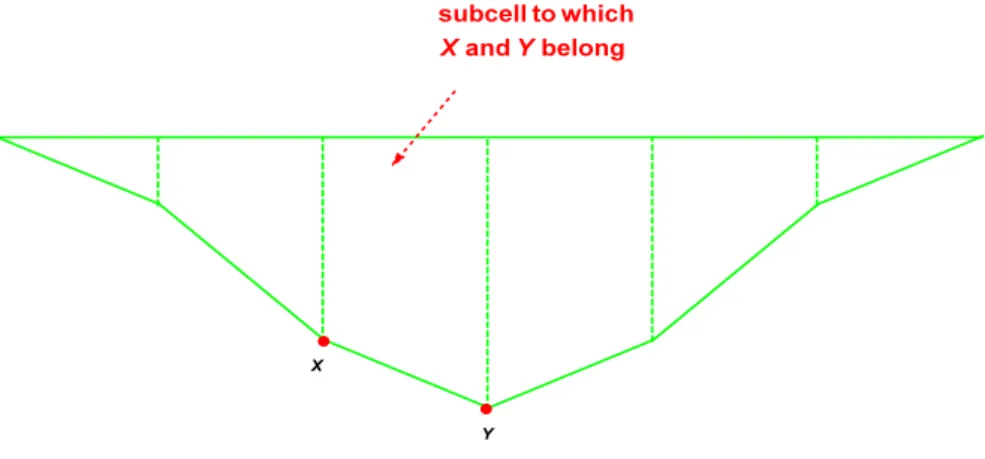
3.1 SubcellsDefinition 3.1. mth−order subcell, m ∈ N⋆, related to a pair of points of the graph ΓW Given a strictly positive integer m, and two points X and Y of Vm such that X∼
mY , we will call
mth−order subcell, related to the pair of points (X, Y ), the polygon, the vertices of which are X, Y , and the intersection points of the edge between the vertices at the extremities of the polygon, i.e. the respective intersection points of polygons of the type Pm,j−1 and Pm,j, 16 j 6 Nbm− 1, on
the one hand, and of the type Pm,j andPm,j+1, 06 j 6 Nbm− 2, on the other hand.
Notation. For any integer j belonging to{0, ..., Nb− 1}, any natural integer m, and any word M of
length m, we set: TM(Pj) = (x (TM(Pj)) , y (TM(Pj))) , TM(Pj+1) = (x (TM(Pj+1)) , y (TM(Pj+1))) Lj,m= x (TM(Pj+1))− x (TM(Pj)) = 1 (Nb− 1) Nbm and: δm = max { 1 (Nb− 1) Nbm , ηm }
Proposition 3.1. Let us denote by:
DW = 2 + ln λ ln Nb
Figure 3: A mth−order subcell, in the case where λ = 1
2, and Nb= 7. the box-dimension (equal to the Hausdorff dimension), of the graph ΓW.
Given a strictly positive integer m, and two points X and Y belonging to Vm, such that X ∼ mY ,
the mth−order subcell, related to the pair of points (X, Y ), is included in the rectangle, whose X and Y are two vertices, of width:
Lj,m=
1 (Nb− 1) Nbm
and height:
ηm = η2−DWLj,m2−DW + η1Lj,m+ η2L2j,m
where the real constants η2−DW, η3−DW, η4−DW are given by :
η2−DW = (Nb− 1)2−DW { 2 1− Nb(DW−2) π2(2 N b− 1) (Nb− 1)2 + 2 π 2(2 N b− 1) (Nb− 1)2 1 NbDW − 1+ 4 π2 (NbDW − 1) } η1 = 8 π2 η2 = 2 π2 (2 Nb− 1)
Proposition 3.2. An upper bound, for the box-dimension of the graph ΓW
For any integer j belonging to {0, 1, . . . , Nb− 1}, and each natural integer m, let us consider the
rectangle, the width of which is:
Lj,m= x (TM(Pj+1))− x (TM(Pj)) =
1 (Nb− 1) Nbm
and the length of which, is:
hj,m=|y (TM(Pj+1))− y (TM(Pj))| 6 ηm
such that the points TM(Pj+1) and TM(Pj+1) are two vertices of .
Let us consider a natural integer Nj,m> Lj,m, and divide Lj,min Nj,mintervals of the same length
Lj,m
Nj,m
. Then:
i. In the case where 1
λ < Nb, the values of hj,m on each of those interval vary at most of: η2−DW ( Lj,m Nj,m )2−DW + η1 Lj,m Nj,m + η2 ( Lj,m Nj,m )2 6 C ( Lj,m Nj,m )2−DW
where C denotes a positive constant which does not depend on Nj,m.
The graph ΓW on Lj,m can be covered by at most:
Nj,m { C ( Lj,m Nj,m )1−DW + 1 } = C L1j,m−DWNj,mDW + Nj,m
squares, the side length of which is Lj,m Nj,m
.
ii. In the case where Nb<
1
λ, the values of hj,m on each of those intervall vary at most of; η2−DW ( Lj,m Nj,m )2−DW + η1 Lj,m Nj,m + η2 ( Lj,m Nj,m )2 6 C Lj,m Nj,m
where C denotes a positive constant which does not depend on Nj,m.
The graph ΓW on Lj,m can be covered by at most:
Nj,m+ 1
squares, the side length of which is Lj,m Nj,m
.
Proof. For any pair of integers (im, j) of{0, ..., Nb− 2}2:
Tim(Pj) = ( xj+ im Nb , λ yj+ cos ( 2 π ( xj+ im Nb )))
For any pair of integers (im, im−1, j) of {0, ..., Nb− 2}3:
Tim−1(Tim(Pj)) = (xj+im Nb + im−1 Nb , λ2yj+ λ cos ( 2 π ( xj + im Nb )) + cos ( 2 π (xj+im Nb + im−1 Nb ))) = ( xj + im Nb2 + im−1 Nb , λ2yj+ λ cos ( 2 π ( xj + im Nb )) + cos ( 2 π ( xj+ im Nb2 + im−1 Nb )))
For any pair of integers (im, im−1, im−2, j) of{0, ..., Nb− 2}4: Tim−2 ( Tim−1(Tim(Pj)) ) = ( xj+ im Nb3 + im−1 Nb2 + im−2 Nb , λ3yj+ λ2 cos ( 2 π (x j+im Nb )) +λ cos ( 2 π ( xj+ im Nb2 + im−1 Nb )) + cos ( 2 π ( xj+ im Nb3 + im−1 Nb2 + im−2 Nb )) )
Given a strictly positive integer m, and two points X and Y of Vm such that:
X ∼
m Y
there exists a wordM of length |M| = m, on the graph ΓW, and an integer j of{0, ..., Nb− 2}2, such
that:
X = TM(Pj) , Y = TM(Pj+1)
Let us write TM under the form:
TM= Tim◦ Tim−1◦ . . . ◦ Ti1
where (i1, . . . , im) ∈ {0, ..., Nb− 1}m.
One has then:
x (TM(Pj)) = xj Nbm + m ∑ k=1 ik Nbk x (TM(Pj+1)) = xj+1 Nbm + m ∑ k=1 ik Nbk and: y (TM(Pj)) = λmy j+ m∑−1 k=1 λm−kcos ( 2 π ( xj Nk b + k ∑ ℓ=0 im−ℓ Nbk−ℓ )) + cos ( 2 π ( xj Nm b + m ∑ k=1 ik Nk b )) y (TM(Pj+1)) = λmy j+1+ m−1∑ k=1 λm−kcos ( 2 π ( xj+1 Nk b + k ∑ ℓ=0 im−ℓ Nbk−ℓ )) + cos ( 2 π ( xj+1 Nm b + m ∑ k=1 ik Nk b ))
|y (TM(Pj+1))− y (TM(Pj))| 6 2 λ m 1− λ π2(2 j + 1) (Nb− 1)2 + 2 m−1∑ k=1 λm−kπ { 2 j + 1 (Nb− 1) Nk b + 2 k ∑ ℓ=0 im−ℓ Nbk−ℓ } π (Nb− 1) Nk b + 2 π 2 (Nb− 1) Nm b ( 2 j + 1 (Nb− 1) Nm b + 2 m ∑ k=1 ik Nk b ) = 2 λ m 1− λ π2(2 j + 1) (Nb− 1)2 + 2 π2λmπ Nb− 1 m∑−1 k=1 { (2 j + 1) λ−k (Nb− 1) N2k b + 2 k ∑ ℓ=0 im−ℓλ−k N2k−ℓ b } + 2 π 2 (Nb− 1) Nm b ( 2 j + 1 (Nb− 1) Nm b + 2 m ∑ k=1 ik Nk b ) + 4 π 2 (Nb− 1) Nm b m ∑ k=1 (Nb− 1) Nk b = 2 λ m 1− λ π2(2 j + 1) (Nb− 1)2 +2 π 2 λmπ Nb− 1 { (2 j + 1) (Nb− 1) λ−1Nb−2(1− λ−m+1Nb−2m+2) 1− λ−1Nb−2 + 2 m ∑ k=1 (Nb− 1) λ−k N2k b 1− Nb−k−1 1− Nb−1 } + 2 π 2 (Nb− 1) Nm b ( 2 j + 1 (Nb− 1) Nm b + 2 m ∑ k=1 (Nb− 1) Nk b ) + 4 π 2 (Nb− 1) Nm b m ∑ k=1 (Nb− 1) Nk b = 2 λ m 1− λ π2(2 j + 1) (Nb− 1)2 + 2 π2λmπ Nb− 1 { (2 j + 1) (Nb− 1) λ−1Nb−2(1− λ−m+1Nb−2m+2) 1− λ−1Nb−2 +2 m ∑ k=1 (Nb− 1) λ−k N2k b 1− Nb−k−1 1− Nb−1 } + 2 π 2 (Nb− 1) Nm b ( 2 j + 1 (Nb− 1) Nm b + 2N −1 b (Nb− 1) (1 − Nb−m+1) 1− Nb−1 ) +4 π 2 Nm b Nb−1(1− Nb−m+1) 1− Nb−1 = 2 λ m 1− λ π2(2 j + 1) (Nb− 1)2 +2 π 2 λmπ Nb− 1 { (2 j + 1) (Nb− 1) λ−1Nb−2(1− λ−m+1Nb−2m+2) 1− λ−1Nb−2 +2 m ∑ k=1 (Nb− 1) λ−k N2k b 1 1− Nb−1 − 2 m ∑ k=1 (Nb− 1) λ−k N2k b Nb−k−1 1− Nb−1 } + 2 π 2 (Nb− 1) Nm b ( 2 j + 1 (Nb− 1) Nm b +2 (Nb− 1) (1 − N −m+1 b ) Nb− 1 ) +4 π 2 (1− Nb−m+1) (Nb− 1) Nm b |y (TM(Pj+1))− y (TM(Pj))| 6 2 λ m 1− λ π2(2 j + 1) (Nb− 1)2 +2 π 2 λm Nb− 1 { (2 j + 1) (Nb− 1) λ−1Nb−2(1− λ−m+1Nb−2m+2) 1− λ−1Nb−2 + 2 m ∑ k=1 (Nb− 1) λ−k N2k b 1 1− Nb−1 −2 m ∑ k=1 (Nb− 1) λ−k N k−1 b 1− Nb−1 } + 2 π 2 (Nb− 1) Nm b ( 2 j + 1 (Nb− 1) Nm b + 2 (1− Nb−m+1) + 2 (1− Nb−m+1) ) 6 2 λm 1− λ π2(2 j + 1) (Nb− 1)2 + 2 π2λm(2 j + 1) (Nb− 1)2 (1− λ−m+1Nb−2m+2) λ N2 b − 1 +4 π2λm1− λ −m+1N−2m+2 b λ N2 b − 1 Nb Nb− 1 − 4 π2 λm1− λ −m+1N−2m+2 b λ N2 b − 1 1 Nb− 1 + 2 π 2 (Nb− 1) Nm b ( 2 j + 1 (Nb− 1) Nm b + 4 (1− Nb−m+1) ) Since: x (TM(Pj+1))− x (TM(Pj)) = 1 (Nb− 1) Nbm
and:
DW = 2 + ln λ ln Nb
, λ = e(DW−2) ln Nb = N(DW−2)
b
one has thus:
|y (TM(Pj+1))− y (TM(Pj))| 6 6 λm { 2 1− λ π2(2 N b− 1) (Nb− 1)2 +2 π 2(2 N b− 1) (Nb− 1)2 1 λ N2 b − 1 + 4 π 2 (λ N2 b − 1) } + 2 π 2 (Nb− 1) Nbm { 4 + 2 Nb− 1 (Nb− 1) Nbm } = em (DW−2) ln Nb { 2 1− e(DW−2) ln Nb π2(2 Nb− 1) (Nb− 1)2 +2 π 2(2 N b− 1) (Nb− 1)2 1 Nb(DW−2)Nb2− 1 + 4 π 2 Nb(DW−2)Nb2− 1) } + 2 π 2 (Nb− 1) Nbm { 4 + 2 Nb− 1 (Nb− 1) Nbm } = Nbm (DW−2) { 2 1− Nb(DW−2) π2(2 N b− 1) (Nb− 1)2 +2 π 2(2 N b− 1) (Nb− 1)2 1 Nb(DW−2)N2 b − 1 + 4 π 2 (Nb(DW−2)N2 b − 1) } + 2 π 2 (Nb− 1) Nbm { 4 + 2 Nb− 1 (Nb− 1) Nbm } = Nbm (DW−2) { 2 1− Nb(DW−2) π2(2 Nb− 1) (Nb− 1)2 + 2 π 2(2 N b− 1) (Nb− 1)2 1 NbDW − 1+ 4 π2 (NbDW − 1) } + 2 π 2 (Nb− 1) Nbm { 4 + 2 Nb− 1 (Nb− 1) Nbm } = L2j,m−DW (Nb− 1)2−DW { 2 1− Nb(DW−2) π2(2 Nb− 1) (Nb− 1)2 +2 π 2(2 N b− 1) (Nb− 1)2 1 NbDW − 1+ 4 π2 (NbDW − 1) } +2 π2Lj,m {4 + (2 Nb− 1) Lj,m} This way:
ηm = ( 1 Nm b )2−DW { 2 1− Nb(DW−2) π2(2 Nb− 1) (Nb− 1)2 + 2 π 2(2 N b− 1) (Nb− 1)2 1 NbDW − 1+ 4 π2 (NbDW − 1) } + 2 π 2 (Nb− 1) Nbm { 4 + (2 Nb− 1) ( 1 (Nb− 1) Nbm )}
3.2 Effective resistance metric
Property 3.3. The space dom ∆, modulo constant functions, is a Hilbert space, included in the space of continuous functions on the graph ΓW, modulo constant functions.
Definition 3.2. Effective resistance metric, on the graph ΓW
Given a pair of points (X, Y ) of the graph ΓW, we define, as in [Str03], the effective resistance metric between the points X and Y , by:
RΓW(X, Y ) =
{
min
{u | u(X)=0,u(Y )=1}E(u)
}−1
In an equivalent way, RΓW(X, Y ) may be defined as the minimum value of the real numbers R such
that, for any function u of dom ∆:
|u(X) − u(Y )|26 R E(u)
Definition 3.3. Metric, on the graph ΓW
Let us define, on the graph ΓW, the distance dΓW defined, for any pair of points (X, Y ) of ΓW, by:
dΓW(X, Y ) =
{
min
{u | u(X)=0,u(Y )=1}E(u, u)
}−1
Remark 3.1. As it is explained in [Str06], one may note that the minimum min
{u | u(X)=0,u(Y )=1} E(u)
is reached when the function u is harmonic on the complement set, in ΓW, of the set{X} ∪ {Y } (we re-call that, by definition, a harmonic function u on ΓWminimizes the sequence of energies(EΓWm(u, u)
)
m∈N.
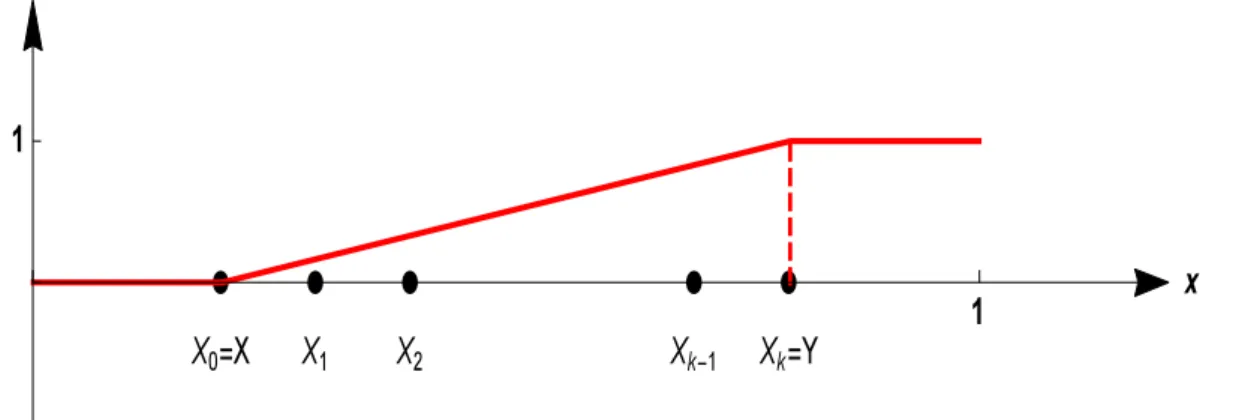
In order to fully apprehend and understand the intrinsic meaning of these functions, one might reason by analogy with the unit interval [0, 1]. In this case, one will note that, given two points X and Y of [0, 1] such that X < Y , the function u is affine by pieces, taking the value zero on [0, X], and the value 1 on [Y, 1] (see the illustration on the following figure):
∀ t ∈ [0, 1] : u(t) = t− X Y − X
Figure 4: The graph of the function u where the value min{u | u(X)=0,u(Y )=1} E(u) is reached.
Let us denote by m the natural integer such that: X ∼
m Y
One may introduce, the, for any integer p, the sequence of points (Xj)06j62p such that:
X0 = X , X2p= Y
and, for any integer j such that 0 < j < 2p− 1:
Xj ∈ Vp+1 , Xj ∼ p+1Xj+1
In the case of the unit interval, the normalization constant is: r−1= 1
2 One has then:
E(u, u) = lim p→+∞Ep(u, u) = lim m→+∞r−pEΓWp(u) = lim p→+∞ ∑ (X,Y )∈ V2 p, X∼pY r−p (u|Vp(X)− u|Vp(Y ))2 = lim p→+∞ ∑ (X,Y )∈ V2 p, X∼ pY 1 2p ( u|Vp(X)− u|Vp(Y ))2 = lim p→+∞ k−1 ∑ j=0 1 2p ( u ( X + j 2p ) − u ( X +j + 1 2p ))2 = ∫ Y X dt (Y − X)2 = 1 Y − X If dRdenotes the usual Euclidean distance on R:
∀ (X, Y ) ∈ R2 : d
R(X, Y ) =|Y − X| one has then:
min
{u | u(X)=0,u(Y )=1}E(u) =
1 dR(X, Y )
Let us now consider, more generally, a fractal domainF, in an Euclidean space of dimension d ∈ N⋆, equipped with the distance dRd. If, one has, in advance, defined an energy onF, it is worth searching
wether there exists a real number β such that: ∀ (X, Y ) ∈ F2 : ( min {u | u(X)=0,u(Y )=1} E(u) )−1 ∼ (dRd(X, Y ))β
In the case of the Sierpi`nski gasketSG (we refer to [?]), Robert S. Strichartz lays the emphasis upon the fact that, given X ∼
m Y , one has: min {u | u(X)=0,u(Y )=1} E(u) . r m SG = ( 3 5 )m
This also corresponds thus to the order of the diameter of the mth−order cells.
Since the Sierpi`nski gasket SG is obtained from the initial triangle of diameter 1 by means of three contractions, the respective ratios of which are equal to 1
2, one has simply to look the real number βSG such that: ( 1 2 )m βSG = ( 3 5 )m
This leads to:
βSG = ln
5 3
ln 2
Definition 3.4. Dimension of the graph ΓW, in the effective resistance metric
The dimension of the graph ΓW, in the effective resistance metric, is the strictly positive num-ber dGammaW such that, given a strictly positive real number r, and a point X ∈ ΓW, for the X−centered
ball of radius r, denoted byBr(X):
µ (Br(X)) = rdΓW
Proposition 3.4. The dimension of the graph ΓW, in the effective resistance metric, is given by: i. First case: λ > 1 Nb . dΓW = lnNb λ ln Nb
ii. Second case: λ < 1 Nb
.
dΓW = 2
Remark 3.2. Once again, it is worth having a look at the case of the Sierpiński gasket. Robert S. Strichartz stars from the fact that the measure of mth−order cells is 1
3m. Two consecutive points x and y are
such that, for the effective resistance metric
d(x, y)∼ (
3 5
)m
For the self-similar measure µSG, which affects the value 1
3m to each m
th−order cell, one has simply
to look for the real number dSG such that: ( 3 5 )m dSG = 1 3m
which leads to:
dSG = ln 3 ln53
One may then deduce from the above an estimate, for the effective resistance metric, of the measure of a X−centered ball of radius r, denoted by Br(X):
µSG(Br(x)) = rdSG
Let us now go back to the graph ΓW.
Given a natural integer m, and two points X and Y such that X ∼
m Y :
min
{u | u(X)=0,u(Y )=1} E(u) . r
−m = Nm b
For the detailed calculations which enable one to obtain the normalization constants, we refer to [?]. For the self-similar measure ˜µ introduced in the above, each mth−order cell, i.e. each simple poly-gonPm,j, 06 j 6 Nbm− 1, with Nb sides and Nb vertices, has a measure of the order of:
(Nb− 1)
ηm Nbm The points X and Y such that X∼
mY belong to a m
th−order subcell, which is the intersection of
a simple polygon Pm,j, 06 j 6 Nbm− 1, with the rectangle of which X and X are two vertices, of
width η
m
Nbm, and heigth η
m. This subcell a has a measure, the order of which is thus:
ηm
Nbm i. First case: λ > 1
Nb
.
One has simply to look for the real number dΓW such that:
Nbm dΓW = λ m Nbm which yields: dΓW = lnNb λ ln Nb
ii. Second case: λ < 1 Nb
.
One has simply to look for the real number βΓW such that:
Nbm dΓW = 1 Nb2m which yields:
dΓW = 2
4
Detailed study of the spectrum of the Laplacian
As exposed by R. S. Strichartz in [Str06], one may bear in mind that the eigenvalues can be grouped into two categories:
i. initial eigenvalues, which a priori belong to the set of forbidden values (as for instance Λ = 2) ; ii. continued eigenvalues, obtained by means of spectral decimation.
We present, in the sequel, a detailed study of the spectrum of ∆, in the case where Nb = 3, which can
be easily extend to higher values of the integer Nb.
4.1 Eigenvalues and eigenvectors of ∆1
Let us recall that the vertices of the graph ΓW1 are:
P0 , T0(P1) , T0(P2) , T1(P0)
P1 , T1(P2) , T2(P0) , T2(P1) , P2
One may note that:
Card (V1\ V0) = 4
Let us denote by u an eigenfunction, for the eigenvalue−Λ. For the sake of simplicity, we set:
u (T0(P1)) = a ∈ R , u (T0(P2)) = b ∈ R , u (T2(P0)) = c ∈ R , u (T2(P1)) = d ∈ R
One has then:
u(P0)− a + b − a = −Λ a a− b + u(P1)− b = −Λ b u(P1)− c + d − c = −Λ c c− d + u(P2)− d = −Λ d
One may note that the only "Dirichlet eigenvalues", i.e. the ones related to the Dirichlet problem: u|V0 = 0 i.e. u(P0) = u(P1) = u(P2) = 0
Figure 5: Successive values of an eigenfunction on V1, in the case where Nb= 3.
are obtained for:
b = −(Λ − 2) a a = −(Λ − 2) b d = −(Λ − 2) c c = −(Λ − 2) d i.e.: b = (Λ− 2)2b a = (Λ− 2)2a d = (Λ− 2)2d c = (Λ− 2)2c The forbidden eigenvalue Λ = 2 cannot thus be a Dirichlet one.
Let us consider the case where:
(Λ− 2)2= 1 i.e.
Λ = 1 or Λ = 3 The value Λ = 1 leads to:
a = b , c = d
which yields a two-dimensional eigenspace. The multiplicity of the eigenvalue Λ = 3 is 2.
For the eigenvalue Λ = 3:
The eigenspace, for the eigenvalue 3, has dimension 2. The multiplicty of the eigenvalue Λ = 3 is 2. Since the cardinal of V1\ V0 is:
NS
1 − Nb = 2 Nb− 2 = 4
one may note that we have the complete spectrum.
4.2 Eigenvalues of ∆2
Let us now look at the spectrum of ∆2. For the sake of simplicity, we will denote by a, b, c, d, e, f , g, h,
the successive values of an eigenfunction at the Nb2− 1 points between P0and P1, and by a′, b′, c′, d′, e′, f′, g′, h′,
the successive values of an eigenfunction at the Nb2− 1 points between P1 and P2, as it appears on the
following figure.
Figure 6: Successive values of an eigenfunction on V2, in the case where Nb= 3.
One has then:
(2− Λ) a = −u(P0)− b (2− Λ) b = −c − a (2− Λ) c = −b − d (2− Λ) d = −c − e (2− Λ) e = −d − f (2− Λ) f = −e − g (2− Λ) g = −f − h (2− Λ) h = −g − u(P1) and:
(2− Λ) a′ = −u(P1)− b′ (2− Λ) b′ = −c′− a′ (2− Λ) c′ = −b′− d′ (2− Λ) d′ = −c′− e′ (2− Λ) e′ = −d′− f′ (2− Λ) f′ = −e′− g′ (2− Λ) g′ = −f′− h′ (2− Λ) h′ = −g′− u(P2)
One may note that the only Dirichlet eigenvalues, in the case where:
u|V1 = 0 i.e. u(P0) = u(P1) = u(P2) = c = f = c′= f′ = 0
are obtained for: (2− Λ) a = −b (2− Λ) b = −c − a 0 = −b − d (2− Λ) d = −e (2− Λ) e = −d 0 = −e − g (2− Λ) g = −h (2− Λ) h = −g and (2− Λ) a′ = −b′ (2− Λ) b′ = −c′− a′ 0 = −b′− d′ (2− Λ) d′ = −e′ (2− Λ) e′ = −d′ 0 = −e′− g′ (2− Λ) g′ = −h′ (2− Λ) h′ = −g′ i.e.: (2− Λ) a = −b { 1− (2 − Λ)2}a = −c 0 = −b − d (2− Λ) d = −e (2− Λ)2e = e 0 = −e − g (2− Λ)2h = h (2− Λ) h = −g and (2− Λ) a′ = −b′ { 1− (2 − Λ)2}a′ = −c′ 0 = −b′− d′ (2− Λ) d′ = −e′ (2− Λ)2e′ = e′ 0 = −e′− g′ (2− Λ)2h′ = h′ (2− Λ) h′ = −g′ The forbidden eigenvalue Λ = 2 is not therefore a Dirichlet one.
Let us consider the case where:
(Λ− 2)2= 1 i.e.
Λ = 3 or Λ = 1 For Λ = 1, one has:
a = −b c = 0 d = −b = a e = −d = a d = −e = −a g = −e = −a h = −g = e = a and a′ = −b′ c′ = 0 d′ = −b′ = a′ e′ = −d′ = a′ d′ = −e′ = −a′ g′ = −e′ = −a′ h′ = −g′ = e′ = a′
The eigenspace, for Λ = 1, has thus dimension 2. The multiplicity of the eigenvalue Λ = 1 is 2. For Λ = 3: a = b c = 0 d = −b = −a e = d = −a g = −e = a h = g = a and a′ = b′ c′ = 0 d′ = −b′ = −a′ e′ = d′ = −a′ g′ = −e′ = a′ h′ = g′ = a′
The eigenspace, for Λ = 3, has thus dimension 2. The multiplicity of the eigenvalue Λ = 3 is 2. Let us now look at the continued eigenvalues, i.e. the ones obtained from the eigenvalues Λ1 = 1
and Λ1= 3 by means of spectral decimation:
Λ2 = ϕ−1 ( (ϕ (Λ1)) 1 Nb ) = { (ϕ (Λ1)) 1 Nb + 1 }2 (ϕ (Λ1)) 1 Nb = −2 + Λ1− ε √ {Λ1− 2}2− 4 2 1 Nb + 1 2 −2 + Λ1− ε √ {Λ1− 2}2− 4 2 1 Nb
where ε ∈ {−1, 1}, for the values:
Λ1 ∈ {1, 3}
As in [Str06], let us get rid, temporarily, of the Dirichlet conditions. We have thus: u(P0) + b = −(Λ − 2) a a + c = −(Λ − 2) b b + d = −(Λ − 2) c e + f = −Λ d e + g = −(Λ − 2) f f + h = −(Λ − 2) g g + u(P1) = −(Λ − 2) h and u(P1) + b′ = −(Λ − 2) a′ a′+ c′ = −(Λ − 2) b′ b′+ d′ = −(Λ − 2) c′ e′+ f′ = −Λ d′ e′+ g′ = −(Λ − 2) f′ f′+ h′ = −(Λ − 2) g′ g′+ u(P2) = −(Λ − 2) h′
For the initial eigenvalue Λ1 = 1, it is worth noticing that its restriction to V1\ V0 must satisfy the
eigensystem associated to the eigenvalue Λ1 = 1, i.e.:
{ u(P0) + f = −(Λ1− 2) c u(P1) + c = −(Λ1− 2) f and { u(P1) + f′ = −(Λ1− 2) c′ u(P2) + c′ = −(Λ1− 2) f′ or: { u(P0) + f = c u(P1) + c = f and { u(P1) + f′ = c′ u(P2) + c′ = f′ i.e.:
For u(P0) = u(P1) = u(P2) = 0, it works, and the Dirichlet conditions appear to be satisfied. One has then: b = −(Λ − 2) a c = {−1 + (Λ − 2)2}a d = (Λ− 2){1−{1− (Λ − 2)2}}a e + f = −Λ (Λ − 2){1−{1− (Λ − 2)2}} a e = (Λ− 2) {1−{−1 + (Λ − 2)2}} h f = {−1 + (Λ − 2)2}h g = −(Λ − 2) h and b′ = −(Λ − 2) a′ c′ = {−1 + (Λ − 2)2}a′ d′ = (Λ− 2){1−{1− (Λ − 2)2}} a′ e′+ f′ = −Λ (Λ − 2) {1−{1− (Λ − 2)2}}a′ e′ = (Λ− 2) {1−{−1 + (Λ − 2)2}}h′ f′ = {−1 + (Λ − 2)2}h′ g′ = −(Λ − 2) h′ We obtain thus an eigenspace, the dimension of which is 4.
For the eigenvalue Λ1 = 1, the spectral decimation spectral leads to:
( 2− Λ2+ ε2ρ (ω2)2 ei θω2 2 )Nb = 1 + ε1 √ 3 ei π2 2 which leads to the double eigenvalue:
Λ2 = 2 + cos π 9 + √ 3 sinπ 9
For the eigenvalue Λ1 = 3, the spectral decimation leads to the double eigenvalue:
Λ2= 2
{
1 + cosπ 9
}
Since the cardinal of V2\ V1= 12 is:
NS
2 − N1S = 2 Nb2+ Nb− 2 − (3 Nb− 2) = 12
one may note that we have the complete spectrum.
4.3 Eigenvalues of ∆3
As previously, one can easily check that the forbidden eigenvalue Λ = 2 is not therefore a Dirichlet one.
One can also check that Λ3 = 1 and Λ3= 3 are eigenvalues of ∆3, both with multiplicity 2.
From: Λ2= 2 { 1 + cosπ 9 }
the spectral decimation leads then to the quadruple eigenvalue: Λ3= 4 cos2 π 27 From: Λ2 = 2 + cos π 9 + √ 3 sinπ 9 the spectral decimation leads then to the quadruple eigenvalue:
Λ3= 4 cos2
π 54
4.4 Eigenvalues of ∆m, m ∈ N, m > 4
As previously, one can easily check that the forbidden eigenvalue Λ = 2 is not therefore a Dirichlet one.
One can also check that Λm = 1 and Λm = 3 are eigenvalues of ∆m, both with multiplicity 2.
By induction, one may note that, due to the spectral decimation, the initial eigenvalue Λ1 = 1 gives
birth, at this mth step, to an eigenvalue Λm, of multiplicity 2m−1. In the same way, the initial
eigen-value Λ1 = 3 gives birth, at this mth step, to an eigenvalue Λm, of multiplicity 2m−1.
Results are summarized in the following array:
Initial eigenvalue Λ1 continued eigenvalue Λ2 continued eigenvalue Λ3 continued eigenvalue Λ4
1 2 + cosπ 9 + √ 3 sinπ 9 4 cos 2 π 27 4 cos 2 π 81 3 2 { 1 + cosπ 9 } 4 cos2 π 54 2 { 1 + cos π 81 }
Property 4.1. Let us introduce:
Λ = lim
m→+∞N m b Λm
One may note that, due to the definition of the Laplacian ∆, the limit exists.
4.5 Eigenvalue counting function
Definition 4.1. Eigenvalue counting function
Let us introduce the eigenvalue counting function, related to ΓW \ V0, such that, for any positive
number x:
NΓW\V0(x) = Card{Λ Dirichlet eigenvalue of −∆ : Λ 6 x}
Property 4.2. Given a strictly positive integer, the cardinal of Vm\ Vm−1 is:
NS
m− NmS−1 = 2
(
Nbm−1− Nbm−2) The highest eigenvalue is:
Nbm× 3 This leads to:
NΓW(Nm
b × 3) =
(
Nbm−1− Nbm−2) If one looks for an asymptotic growth rate of the form
NΓW(x)∼ xα
one obtains:
α = 1 By following [Str06], one may note that the ratio
NΓW(x)
x
is bounded above and away from zero, and admits a limit along any sequence of the form C Nbm, C > 0, m ∈ N⋆. This enables one to deduce the existence of a periodic function g, the period of which is equal to ln Nb,
discontinuous at the value 3, such that: lim x→+∞ { NΓW(x) x − g(ln x) } = 0
Remark 4.1. Existing results of J. Kigami and M. Lapidus [KL03], and also of R. S. Strichartz [Str06], yield: NΓW(x) = G(x) xαΓW +O(1) with: αΓW = dΓW dΓW + 1 = lnNb λ ln Nb lnNb λ ln Nb + 1 where: dΓW = lnNb λ ln Nb
is the dimension of the graph ΓW for the resistance metric.
References
[BBR17] K. Barańsky, B. Bárány, and J. Romanowska. On the dimension of the graph of the classical Weierstrass function. Advances in Math., 2017.
[BD85a] M. F. Barnsley and S. Demko. Iterated function systems and the global construction of fractals. The Proceedings of the Royal Society of London, 1985.
[BD85b] A. Beurling and J. Deny. Espaces de Dirichlet. i. le cas élémentaire. Annales scientifiques de l’É.N.S. 4 e série, 1985.
[BL80] M.V. Berry and Z. V. Lewis. On the Weierstrass-Mandelbrot function. Proc. R. Soc. Lond, 1980.
[Dav17] Claire David. Laplacian, on the graph of the Weierstrass function, arxiv:1703.03371, 2017. [DR16] Cl. David and N. Riane. Formes de Dirichlet et fonctions harmoniques sur le graphe de la
fonction de Weierstrass, hal-01421453, 2016.
[Fal85] K. Falconer. The Geometry of Fractal Sets. Cambridge University Press, 1985.
[FOT94] M. Fukushima, Y. Oshima, and M. Takeda. Dirichlet forms and symmetric Markov processes. Walter de Gruyter & Co, 1994.
[FS92] M. Fukushima and T. Shima. On a spectral analysis for the Sierpiński gasket. Potential Anal, 1992.
[FS11] Z. Feng and Y. Song. Some properties of the Sierpiński tetrahedron. International Journal of Nonlinear Sciencel, 2011.
[Har11] G. Hardy. Theorems connected with Maclaurin’s test for the convergence of series. The Proceedings of the Royal Society of London, 1911.
[HMC13] S. A. Hernández and F. Menéndez-Conde. Some properties of the Sierpiński tetrahedron. Abstract and Applied Analysis, 2013.
[Hun98] B. Hunt. The Hausdorff dimension of graphs of Weierstrass functions. Proc. Amer. Math. Soc., 1998.
[Hut81] J. E. Hutchinson. Fractals and self similarity. Indiana University Mathematics Journal, 1981. [Kel17] G. Keller. A simpler proof for the dimension of the graph of the classical Weierstrass function.
Ann. Inst. Poincaré, 2017.
[Kig89] J. Kigami. A harmonic calculus on the Sierpiński spaces. Japan J. Appl. Math., 1989. [Kig93] J. Kigami. Harmonic calculus on p.c.f. self-similar sets. Trans. Amer. Math. Soc., 1993. [Kig98] J. Kigami. Distributions of localized eigenvalues of Laplacians on post critically finite
self-similar sets. J. Funct. Anal., 1998.
[Kig03a] J. Kigami. Harmonic analysis for resistance forms. Journal of Functional Analysis, 2003. [Kig03b] J. Kigami. Harmonic analysis for resistance forms. Journal of Functional Analysis, 2003. [KL03] J. Kigami and M. Lapidus. Weyl’s problem for the spectral distribution of laplacians on p.c.f.
self-similar fractalss. Communications in Mathematical Physics, 2003.
[Man77] B. B. Mandelbrot. Fractals: form, chance, and dimension. San Francisco: Freeman, 1977. [RSS81] T. Zhang R. S. Strichartz, A. Taylor. Densities of self-similar measures on the line.
Experi-mental Mathematics, 1981.
[Sab97] C. Sabot. Existence and uniqueness of diffusions on finitely ramified self-similar fractals. Annales scientifiques de l’É.N.S. 4 e série, 1997.
[Shi91] T. Shima. On eigenvalue problems for the random walks on the Sierpiński pre-gasket. Japan J. Indus. Appl. Math., 1991.
[Str99] R. S. Strichartz. Analysis on fractals. Notices of the AMS, 1999. [Str01] R. S. Strichartz. Analysis on fractals. Notices of the AMS, 2001.
[Str06] R. S. Strichartz. Differential Equations on Fractals, A tutorial. Princeton University Press, 2006.
[Str12] R. S. Strichartz. Exact spectral asymptotics on the Sierpiński gasket. Proc. Amer. Math. Soc., 2012.
[Tit77] E. C. Titschmarsh. The theory of functions, Second edition. Oxford University Press, 1977. [Wei72] K. Weierstrass. Über continuirliche funktionen eines reellen arguments, die für keinen werth
des letzteren einen bestimmten differentialquotienten besitzen, in karl weiertrass mathematis-che werke, abhandlungen ii. Akademie der Wissenchaften am 18 Juli 1872, 1872.