Design and Experimental Analysis of Legged
Locomotive Robots
by
Timothy J. Villabona
Submitted to the Department of Mechanical Engineering in partial fulfillment of the requirements for the degree of
Bachelor of Science in Mechanical Engineering at the
MASSACHUSETTS INSTITUTE OF TECHNOLOGY
MASSACHUSETTS INST UTE
OF TECHNOLOGY
SEP 16 2009
LIBRARIES
ARCHIVES
Author .. June, 2009@Massachusetts Institute of Technology, 2009. All rights reserved.
Department of Mechanical Engineering 11th May 2009
(Th
Certified by.. ... .. . ... ... ...
Russell L. Tedrake Professor, Department of Electrical Engineering and Computer Science Thesis Advisor
Accepted by ...--. ...
John Lienhard V Collins Professor of Mechanical Engineering Chairman, Undergraduate Thesis Committee
Design and Experimental Analysis of Legged Locomotive Robots
by
Timothy J. Villabona
Submitted to the Department of Mechanical Engineering on 11th May 2009, in partial fulfillment of the
requirements for the degree of
Bachelor of Science in Mechanical Engineering
Abstract
In this thesis, I present the design and motion-capture analysis of two previously well-studied dynamic-walking machines, the rimless wheel and the compass gait robot. These robots were the basis for my undergraduate research at the Computer Science/Artificial Intelli-gence Laboratory (CSAIL) at the Massachusetts Institute of Technology. The rimless wheel is a real-world physical realization built to compare to a long-analyzed model, the simplest example of passive dynamic walking. Despite the seemingly deterministic model, undeniable experimental evidence for unpredictable stochasitic behavior is observed. The compass gait is the second iteration of a previous design by Dr. Fumiya Iida in my laboratory. Both ma-chines are among the most fundamental walking models, and are important for developing energy-efficient dynamic walkers.
Thesis Supervisor: Russell L. Tedrake
Professor, Department of Electrical Engineering and Computer Science
Approved by: John Lienhard V
Collins Professor of Mechanical Engineering Chair, Undergraduate Thesis Committee
Acknowledgments
I'd like to thank Russ Tedrake of the MIT Computer Science and Artificial Intelligence Lab-oratory. As a mechanical engineering undergraduate, much of his work in control theory and locomotion exceeded my mental latitudes in my time spent working in his laboratory. Though much of his work still lies beyond my analytical reach, I've gained valuable design experience and learned of the amazing robots that can be created by applying online learning and simple mechanical control to legged locomotion. Thrishantha Nanayakkara of Harvard University provided guidance and support through his one-on-one assistance developing the numerical analysis employed for data analysis and his part in developing the analytic models for the rimless wheel. His MATLAB knowledge proved invaluable.
I'd like to thank Rick Cory for his expertise in developing the motion-capture program mod-els, and John W. Roberts for his assistance with the high-speed video hardware and software. Thanks also to Stephen Proulx and Fumiya lida for providing helpful insight and ideas for the construction of both the rimless wheel and compass gait.
1
Introduction
1.1
Passive Dynamic Walking
In the late 1980s, Tad McGeer introduced the style of robot locomotion known as passive dynamic walking [4]. These machines are completely passive, meaning that they derive their kinetic energy from gravitational potential energy. The robots must walk down a (slight) decline, and the conversion of potential to kinetic energy drives their motion. Steady-state is attained by the balance of energy losses in the foot collisions and friction either at the foot-floor interface or internal joint friction.
Passive locomotion is the best method for initial study of foot-ground interactions because no external actuation can suppress natural behaviors intrinsic to the system. The hope of passive dynamic walking research is that its analysis might aid in the development of more complex walkers. By actuating some degrees of freedom and adding control, amazing walkers can emerge that take advantage of the energy efficiency of passive walkers and make their gaits more useful with control. Furthermore, these walkers aim to emulate the motions of the human gait. Insight into these motions has important benefits for prosthetics development, more ergonomic footwear, and improve neuromuscular rehabilitation [1].
1.2
Applying Control to Passive Dynamics
Figure 1 shows an example of bridging this gap between passive and simple actuated robots, designed by Russ Tedrake of MIT. The left robot is a passive dynamic walker which walks down a small ramp following a small sidways push. The robot rocks onto a single stance leg, while the other leg swings forward down the ramp. The robot lands on this swing leg, while the previous stance leg swings forward. The cycle repeats, converting gravitational energy to kinetic energy of the swinging foot and energy lost to foot-ground friction and inelastic collisions. This robot has but one passive pin joint at the hip. This waddling gait is the
Figure 1: The robot on the left is a simple passive dynamic walker-completely unactuated. The robot on the right is an actuated version of the same robot.
simplest representation of stable three-dimensional walking. The right robot is an actuated version of the same passive walker, capable of walking on flat terrain. This intelligent robot learns a control algorithm to restore energy to the robot that is lost to the collisions and friction, which would have been otherwise restored by gravity [2].
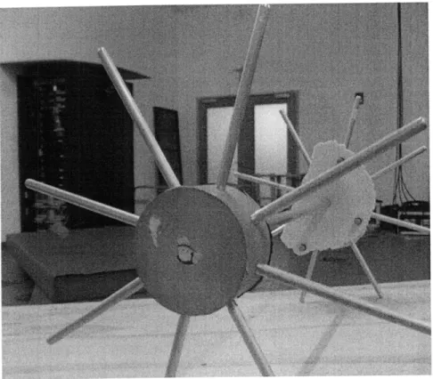
The goals of my undergraduate research were to design and investigate the behavior of a passive walker, the rimless wheel [1], and design a new minimally-actuated walker, the
2
Rimless Wheel
2.1
Background and Model
The rimless wheel (RW) is the simplest model of passive dynamic walking. The canonical model has no hinges, only rigid legs and a central point mass. This model has been analyzed in [2,4]. This model provides the most basic and essential features of walking-a discrete set of ground contact points with significant energy conversions at the collisions ending each cycle. Figure 2 shows a modified version of the canonical model for the rimless wheel. The
(M + 4m)189
M + 4m)g
Figure 2: The rimless wheel model.
modifications are made in order to better rectify the model with the physical embodiment of the constructed rimless wheel. Most notably, rather than a point mass, a more accurate mass distribution is needed. The body is now a central hub, and the mass of the legs is accounted for. The central hub of mass M has n equal-length legs protruding from it. Between each step, the mass of the hub gains kinetic energy as it is converted from gravitational potential energy. At each discrete step, the rimless wheel loses angular velocity, both from conservation
of angular momentum and from energy lost to foot-ground friction and vibrations dissipated through the floor and the rimless wheel. The original model introduced by McGeer in [3] treats the weight transfer phase (leg-to-leg) as slipless and inelastic. Maintaining these assumptions, we introduce a coefficient of restitution to model the impacts. Let point O be the datum of potential energy. Model one pair of opposite legs as a rod passing through the central hub. Let I be the moment of inertia of one pair of legs. Let M >> m. The kinetic energy of the rimless wheel is given by
1 4
L= -
1(M +
4m)1202 + -1 2,2 2
while the gravitational torque is
(M + 4m)gl cos 0. (2)
Rewriting these two dynamics as a sum ( of generalized torques,
d OL L
dt= ( ) (3)
gives
[(M + 4m)12 + 41] 0 - (M + 4m)gl cos 0. (4)
As this is passive locomotion we have no further forces or torques and may set our expression = 0. This gives an ordinary differential equation of the form
C = f(x, ~) (5)
where x = [, ] and 0b represents the physical system parameters. As described earlier, we may assume from intuition that the impacting "steps" result in a loss of kinetic energy dissipated in vibrations sent through the floor and body of the rimless wheel. We can model
this idea as
+ = e6-, e < 1,
where e is the loss coefficient and [-, +Jindicate variables immediately before and after a collision, respectively.
When applied numerically from collision to collision, we arrive at a steady-state value for 0, that is, the system recuperates energy between each collision such that
k =
-
n+1, (7)where n indicates a collision. This is a somewhat crude model of the rimless wheel dynamics; we shall see that the model must be expanded to include an element of stochasticity.
2.2
Experimental Procedure
Initial Steep
Ramp
Figure 4: The rimless wheel experimental setup.
Our rimless wheel was constructed of aluminum. Because a single rimless wheel would be hopelessly unstable in the axial direction (the plane of the page in Fig. 2), two identical rimless wheels were constructed and rigidly bounded by an axle. They were keyed to the axle to ensure leg alignment. On each end of the axle, eight legs of 0.135m were threaded into a central hub of mass 1.39kg. The combined mass of the legs was about L the mass of the central hub. In the first several rounds of trials, the legs tended to come unthreaded and excessively wobbly; springs were added into the holes to keep the legs preloaded against the threads. A ramp of 100 slope and 3.5m length was constructed of standard lumber. All experiments involved the rimless wheel rolling down this ramp with nine motion capture markers affixed to one of the central hubs. One leg was marked and the rimless wheel was released from this grounded leg for all trials. One version of the experiment consisted of releasing the RW from a steeper 450 ramp, allowing it to transfer to the longer flatter ramp (51 trials). The second version of the experiment consisted of the RW released directly on the flatter ramp (48 trials). This gave two distributions of initial velocity and allowed for confident conclusions to be drawn regarding the convergence properties of the RW to steady
state. Both versions of the experimental setup are depicted in Fig. 4.
2.3
Data Analysis
Sixteen cameras recorded the xyz coordinates of the markers at 120Hz. These raw coor-dinates were synthesized using an algorithm derived in [5] to obtain the stepwise angular displacement of the rimless wheel. The accuracy of the motion-capture system is
remark-0.05 Raw Data Savitsky-Golay Filtered
0.04 0.03 0.03 - A 0.02 0.041 oig03 0 0-Y 04 -0.02 -002 --003 12 1.4 1.6 1.8 2 2.2 2.4 2.6 2.8 1 12 14 1.6 1.8 2 22 2.4 time, a time, s
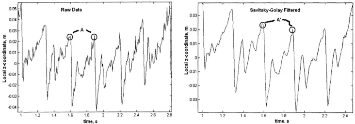
Figure 5: Side-by-side comparison of raw, localized (with the hub center as the origin) z-coordinate data and data cleaned via Savitsky-Golay filtering. Note the preservation of the sharp derivatives (points A and A'), while smoothing out the high-frequency vibrational system noise.
able; with 16 cameras the system is able to track markers with sub-millimeter precision in a 3-meter cubic area. The drawback of such precision is that for these experiments such sensitivity is able to capture the vibrations of the legs, which can make observation of the larger-scale motions of the system difficult. While we are only concerned with the angular velocity of the rimless wheel, the vibrations from impact made it difficult to pin down the angular motions of the rimless wheel from the raw 3-d coordinates. It was clear from video observation that vibrations were sent through the body of the RW as several legs could be seen vibrating. In fact, the original model of the RW had longer legs; the one described in these experiments had shortened legs to help reduce vibrations. Even with markers placed on the central hub, removal of this vibrational "noise" was necessary. Fig. 5 depicts the
typical data recorded from a given trial. A 3rd-degree Savitsky-Golay filter was employed to reduce high-frequency data.
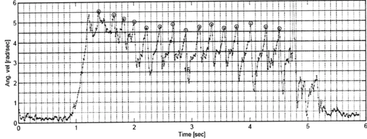
From the data alone, it is difficult to separate the instant of the collisions from bounces and slippage of the feet. Especially for the first few impacts, the RW is susceptible to skip-ping and bouncing along the wood surface. To help differentiate the two, we recorded video at 120Hz and synchronized the video with the angular velocity data. Visual inspection of the video aided in developing algorithms to separate collisions from bounces. The algorithm developed seeks velocity peaks in the range of 450 increments (the predicted rotation angle between impacts). Fig. 6 shows a characteristic motion-capture data trial of the rimless wheel. Note the initial higher-speed impacts from rolling the RW down a steeper ramp, and the settling to a lower, repeated velocity at each impact.
6 i i i i i i i 8 i i { i i i i i i I t i i i i i
1 + i i iL I i i i 4 {i iL4 i w L i L i i i i i
2
i0 1 2 3 4 b 6
Time [sec]
Figure 6: A sample trial of the rimless wheel rolled collision are marked with circles.
down the steeper ramp. The points of
2.4
Discussion of Results
The distributions for collision impact velocities are shown in Fig 7. Note that the faster starts converge to similar velocities to the trials from the regular, less inclined ramp. In both types of trials, the first few collisions are widely varied, yet the speed of the rimless
Impact I s impact 3 2 .51 5 1 2 4 5 6 7 3 . . Impacts 8-11 25. .5 1 2 3 4
impact velocity, iadi's 5 6
rolled from 2. O. 0 2 Ca z 0. 7 s Impact 2 -r ap id ... .... ... . .. ... 5 -convergence to 1 steady-state 5-01 1 2 3 4 5 6 7 3S mpactsmpacts 4-7 2 5 1 5 0 1 2 3 4 5 6 7 .5 Impacts 12-15 2 .5 1 2 3 4 5 6 7 regular ramp
impact velocity, rad/s
Im pact I.. .... • . 5s Impact 3 2 3 s Impacts 8-11 2- 5- 1-2- convergence ... s after several - impacts 3 4 5 6 7 5. Impact 2 2 1 2 3 4 5 6 7 ImpatsImpacts 4-7 2 5 1-Impacts 12-l15
impact velocity, rad!s impact velocity, rad/s
rolled from initial steeper ramp
Figure 7: Histograms of rimless wheel collisions for two types of trials.
1 2
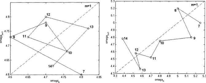
wheel eventually converges to a more consistent value. This convergence takes many more collisions in the trials including the steeper ramp-about 10 collisions versus two for those only involving the shallower ramp. This longer convergence time is likely due to the fact that the rimless wheel takes several collisions to dissipate the excess kinetic energy generated from rolling down the steeper ramp. However, there remains significant variability throughout the trial, even once the rimless wheel has arrived at it's 'steady-state' phase-i.e., where it is as close to conservation of net energy from one collision to the next as it will get. This idea of unpredictability is further illustrated in Fig. 8, which shows the return maps 1 of two consecutive trials. Note how there is no trend of collisions on the line of slope m = 1, nor
omega
n
omegan
Figure 8: Typical return maps of two consecutive trials. Note how there is no similarity in shape, and the inconsistency of angular speeds between identical collisions in both trials.
are there any distinct similarities between the two maps.
1
A return map plots a parameter at a discrete event versus the parameter at the following discrete event-in this case, w(n) vs. w(n+ 1), where n represents each collision. Poevent-ints fallevent-ing on the slope m = 1 imply that
cyclic-wise (not instantaneous) steady-state has been reached, since the system is at the same parameters
These results reveal that there is much more to the story of the dynamics of the rimless wheel than revealed in Eq. 6. Recall that the rimless wheel started from the same initial orientation for all trials. Thus, judging from the return maps of Fig. 8, even if we inspect the location of the same collisions (hence, the same leg impacts), we see a high level of variance. This stochasticity is not entirely surprising, since there are simply too many variables to model accurately the collision dynamics for every possible foot-ground interaction. The grain profile of the wooden ramp at impact, the surface finish of the wood, the imperfections from leg to leg, as well as for the two bounded rimless wheels-these are all factors which affect the interactions of the collision. If we assume that after collision, the next physical interaction the RW has with the environment is the next collision (no further external dis-turbances), then-whatever the source-the net effect of this environmental stochasticity is a
change in vale for the coefficient of restitution e from Eq. 6.
Most modern robots rely on wheeled mechanisms for locomotion, which greatly reduces the element of stochasticity encountered from foot-ground impacts. However, this method of transport also greatly limits the ability of something to traverse anything but flat terrain. Any (relatively) large bumps, steps, or even obstacles such as tall grass or weeds are much more easily traversed with limbs of multiple degrees of freedom. As this is the simplest model of legged walking in a controlled laboratory setting, the stochasticities encountered here may be fundamental to all legged walkers. A predictive learning algorithm to constantly monitor environment might be employed to control limbs to minimize losses or maximize stability.2
2
For in-depth analysis and presentation of novel methods of online learning algorithms, see [Tedrake, 2004].
3
Compass Gait
3.1
Introduction
M
swing leg
>
M stance legFigure 9: Schematic of the compass gait analytic model.
The compass gait is a simple bipedal robot with two legs and a pin joint connecting them at the hip. This is an improvement on the rimless wheel in the sense that it better approximates human locomotion. The state of the robot is described by the position and velocity of its two legs, known as the stance and swing legs. This is a sufficiently simple model such that its dynamics are feasible to model analytically. Furthermore, in rough terrains, its point-approximating feet better enable foot placement control than walkers with larger curved feet [7].
The compass gait and its control solutions have been analyzed extensively-both numer-ically [2,6, 10] and experimentally [7]. The current challenge is controlling the compass gait in rough terrain. The experimental compass gait used in [7] is shown in Fig. 10. In order to maintain stability, the hip was attached to a boom with a set of counterweights. The motor driving the legs was attached coaxially with the boom axis, hanging off the side of the leg assembly. This necessitated another counterweight on the other side of the compass gait to even its rotational inertia, and more weight at the end of the boom to even the masses at both ends of the boom. I undertook the design of a new compass gait with a bisecting angle mechanism to reduce the overall rotational inertia of the compass gait. A bisecting angle
Figure 10: The previous compass gait robot
mechanism has been employed in actuated walker design before [8,9], with the benefit being actuation of both legs while eliminating a degree of freedom.
3.2
New Design
This new compass gait design is shown in Fig. 11. The new design houses the motor between the legs of the robot in order to minimize its torque on the entire assembly. Both legs are free to swing independently of each other without the motor in place, but with the motor connected to the legs via bevel gears, all three bodies are kinematically coupled such that the motor always bisects the angle of the separated legs. The legs are coupled to the shaft as shown in Fig. 12. Both legs are set on bearing sets (a) which are snugly fit onto a central
Figure 11: The new compass gait robot design
shaft passing through the entire assembly (not shown). A press fit was avoided in order to maintain the ability to disassemble the entire robot. The bearings are press fit into the bearing rings (b), as is one bevel gear (c) on the inner side of each leg. This bearing/gear ring is subsequently press fit into the hole at the hip of each leg for attachment to the central shaft. The motor is mounted to the central shaft by an L-shaped bracket, which allows the motor to swing freely so that its effect on the leg swings is minimized. E-clips are used to bind the entire assembly together in the shaft's axial direction. To isolate the motor's shaft from the compliance of the mounting bracket and leg attachments, and to prevent the bevel gears from binding up from such deflections, a flexure coupling is used to couple the motor to the bevel gear train. This coupling has compliance in all but the axial direction, so the motor and bevel gears may shift slightly relative to their nominal orientation while still
Figure 12: Solid modeled exploded view of the leg attachment assembly
providing smooth torque. A bearing block is deemed unnecessary as the motor shaft under this design takes minimal lateral forces-its weight is mostly carried by the central shaft, and its loading is nearly radially symmetric.
3.3
Discussion
It is the hope of the author that this design of the compass gait will improve on the efficiency of the previous design. In passive walkers, efficiency is key-Honda's ASIMO has only roughly
1 the efficiency of humans [2]. Furthermore, this design provides a new experimental model
of legged locomotion and better approximates human locomotion because of its inherent symmetry and lower center of mass. Humans rely heavily on the inertia of their swinging leg while walking. In a sense, the human gait resembles repeated cycles of falling down and catching-though this is complicated by the toe, ankle, and knee joints.
4
Closing Remarks
The walkers discussd in this thesis are two of the most fundamental models of legged lo-comotion. Analysis of the rimless wheel has shown us that stochasticity cannot be ignored even in the simplest, one degree-of-freedom model we can create of legged locomotion. For jointed and other more complicated robots, one can only expect to encounter more variabil-ity, especially in foot-ground interactions and any other external impacts. The compass gait takes us one step closer to fully actuated bipedal locomotion. Possible future expansions of the robot presented here might include knee and ankle joints [7], or the removal of the radial boom to further challenge the development of robust control strategies.
References
[1] T. McGeer (May 1990) "Passive bipedal running," Proc. of the Royal Society of London, vol. 240, no. 1297, pp. 107-134
[2] R. Tedrake (Sep 2004) "Applied optimal control for dynamically stable legged loco-motion," Ph.D. Thesis, Dept. of Electrical Engineering and Computer Science, Mas-sachusetts Institute of Technology.
[3] T. McGeer (Apr 1990) "Passive Dynamic Walking," Int'l Journal of Robotics Research, vol. 9, no. 2, pp. 62-82.
[4] T. McGeer (1993) "Dynamics and Control of Bipedal Locomotion," Journal of
Theoret-ical Biology, no. 163, pp.2 77-3 14.
[5] S. Blostein, T. S. Huang, K. Arun (Sep 1987) "Least-Squares Fitting of two 3-D Point Sets" IEEE Trans. on Pattern Analysis and Machine Intelligence, vol. 9, no. 5, pp. 698-700.
[6] A. Goswami, B. Espiau, A. Keramane (Apr 1996) "Limit cycles and their stability in a passive bipedal gait", Proc. of the 1996 IEEE Int'l Conf. on Robotics and Automation
(ICRA), pp. 246-251.
[7] F. lida, R. Tedrake (2009) "Minimalistic Control of a Compass Gait Robot in Rough Terrain" Proc. of the IEEE/RAS Int'l Conf. on Robotics and Automation (ICRA). [8] Steven Hartley Collins, Andy Ruina (Apr 2005) "A bipedal walking robot with efficient
and human-like gait", Proc. of the 2005 IEEE Int'l Conf. on Robotics and Automation
(ICRA).
[9] Martijn Wisse (Sep 2004) "Essentials of dynamic walking; Analysis and design of two-legged robots," PhD Thesis, Technishe Universiteit Delft.
[10] M.W. Spong, G. Bhatia (Oct 2003) "Further results on control of the compass gait biped," Proc. of the IEEE Int'l Conf. on Intelligent Robots and Systems (IROS), pp. 1933-1938.


