Design and implementation of an indoor mobile navigation system

(1)

Design and Implementation of an Indoor Mobile Navigation

System

by

Allen Ka Lun Miu

B.S., Electrical Engineering and Computer Science, University of California at Berkeley (1999)

Submitted to the Department of Electrical Engineering and Computer Science in partial fulfillment of the requirements for the degree of

Master of Science in Computer Science and Engineering at the

MASSACHUSETTS INSTITUTE OF TECHNOLOGY January 2002

c

Author . . . . Department of Electrical Engineering and Computer Science

January 18, 2002 Certified by . . . . Hari Balakrishnan Assistant Professor Thesis Supervisor Accepted by . . . . Arthur C. Smith Chairman, Department Committee on Graduate Students

(2)

Design and Implementation of an Indoor Mobile Navigation System by

Allen Ka Lun Miu

Submitted to the Department of Electrical Engineering and Computer Science on January 18, 2002, in partial fulfillment of the

requirements for the degree of

Master of Science in Computer Science and Engineering

Abstract

This thesis describes the design and implementation of CricketNav, an indoor mobile navi-gation system using the Cricket indoor location sensing infrastructure developed at the MIT Laboratory for Computer Science as part of Project Oxygen. CricketNav navigates users to the desired destination by displaying a navigation arrow on a map. Both the direction and the position of the navigation arrow are updated in real-time as CricketNav steers the users through a dynamically computed path. To support CricketNav, we developed a modular data processing architecture for the Cricket location system, and an API for accessing loca-tion informaloca-tion. We implemented a least-squares posiloca-tion estimaloca-tion algorithm in Cricket and evaluated its performance. We also developed a rich and compact representation of spa-tial information, and an automated process to extract this information from architectural CAD floorplans.

Thesis Supervisor: Hari Balakrishnan Title: Assistant Professor

(3)

Acknowledgments

I would like to deeply thank my advisor, Hari Balakrishnan, for being my personal navigator who always guided me back on track whenever I am lost. I also thank my mentors Victor Bahl and John Ankcorn for sharing their invaluable advice and experiences.

I thank Bodhi Priyantha for his devotion in refining the Cricket hardware to help make CricketNav possible. I thank the rest of the Cricket team (Dorothy Curtis, Ken Steele, Omar Aftab, and Steve Garland), Kalpak Kothhari, “Rafa” Nogueras, and Rui Fan for their feedback about the design and implementation of CricketServer and CricketNav. My gratitude also goes to Seth Teller, who showed me the way to tackle the map extraction problem.

I would like to acknowledge William Leiserson, who wrote the source code for ma-nipulating UniGrafix files and floorplan feature recognition, and Philippe Cheng, who has contributed some of the ideas used in extracting accessible paths and space boundaries from CAD drawings.

My time spent working on this thesis would not have been nearly as fun without my supportive and playful officemates and labmates: Godfrey (“Whassup yo?”), Kyle (“I gotta play hockey.”), Michel and Magda (“Hey, you know.”, “Hey, you know what?”). I also thank my ex-officemates, Alex, who have shown me the ropes around MIT when I first arrived, and Dave, who always have something interesting to say about anything and everything.

I would like to thank my close friends—Alec Woo, Eugene Shih, Karen Zee, Norman Lee, Ronian Siew, Victor Wen—for their companionship and support.

I dedicate this thesis to my family and my beloved Jie for their unconditional love and encouragement.

(4)

List of Figures

1-1 Screen shot of a navigation application. It shows an navigation arrow in-dicating the user’s current position. The arrow indicates the direction that

leads the user towards the destination. . . 10

1-2 Components required for CricketNav. . . 11

2-1 A person carrying a CricketNav device is in the office 640A so the correct navigation arrow should point downwards. However, small errors in reported coordinate value may cause the navigation arrow to anchor outside the room and point in the wrong direction. . . 14

2-2 The Cricket Compass measures the angle θ with respect to beacon B. . . . 18

2-3 Software architecture for CricketServer. . . 19

2-4 A Cricket beacon pair is used to demarcate a space boundary. The beacons in a beacon pair are placed at the opposite sides of and at equal distance away from the common boundary that they share. There is a beacon pair that defines a virtual space boundary between A₀ and A₁. Each beacon advertises the space descriptor of the space in which the beacon is situated. This figure does not show the full space descriptor advertised by each beacon. 21 2-5 The coordinate system used in Cricket; the beacons are configured with their coordinates and disseminate this information on the RF channel. . . 22

2-6 Experimental setup: Beacon positions in the ceiling of an open lounge area 26 2-7 Sample distribution for all beacons listed in Table 2.1 . . . 26

2-8 Position Error (cm) vs. k using MEAN distance estimates. The speed of sound is assumed known when calculating the position estimate. . . 29

2-9 Position Error (cm) vs. k using MODE distance estimates. The speed of sound is assumed known when calculating the position estimate. . . 29

2-10 Position Error (cm) vs. k using MODE distance estimates and varying m between 4 and 5. The curves labeled UNKNOWN (KNOWN) represent the results obtained from a linear system that assumes an unknown (known) speed of sound. . . 29

2-11 Standard deviations of the results reported in Figure2-10. . . 29

2-12 Position Error (cm) vs. m for k = 1. . . . 30

2-13 Standard deviations of the results reported in Figure2-12. . . 30

2-14 Cumulative error distribution for k = 1 and m = 3, 4. Speed of sound is assumed known. The horizontal line represents the 95% cumulative error. . 31

2-15 Cumulative error distribution for k = 1 and 5 ≤ m ≤ 12. Speed of sound is assumed unknown. The horizontal line represents the 95% cumulative error. 31 2-16 Mean, mode, and standard deviation of the time elapsed to collect one sample from m beacons. . . . 33

(7)

2-17 Mean latency to collect k samples each from m beacons. . . . 33

2-18 Median latency to collect k samples each from m beacons. . . . 33

3-1 Process for floorplan conversion. . . 40

3-2 Components of a doorway in a typical CAD drawing. . . 41

3-3 The figure shows a triangulated floor map, which shows the constrained (dark) and unconstrained (light) segments. For clarity, the unconstrained segments we show are the ones in the valid space only. . . 42

3-4 The figure shows the extracted accessible paths from the same triangulated floor map. The accessible path connects the midpoint of the triangles in valid space. . . 42

3-5 The primal and dual planar graph consisting of a single primal triangle. . . 44

3-6 The corresponding quad edge representation for the primal triangle. . . 44

3-7 The data structure representing quadedge α. . . . 44

4-1 CricketNav prototype. The snapshot is shown in 1:1 scale to the size of a typical PDA screen (320x240 pixels). . . 47

4-2 A correction arrow appears when the user wanders off the wrong direction. 48 4-3 Two possible paths leading to destination. The solid path is generally preferred. 50 4-4 A local path (light) is constructed when the user wanders away from the original path (dark). . . 50

4-5 Three arrows pointing upwards. The arrow orientations are left-turn, straight, right-turn. . . 50

4-6 The shape and direction of the path between points P and Q are used to determine the orientation and direction of the navigation arrow. . . 51

(8)

List of Tables

2.1 Experimental setup: Beacon coordinates (in cm) . . . 25

(9)

Chapter 1

Introduction

1.1 Motivation

Imagine that it is your first time visiting the Sistine Chapel and you have a strong desire to see Michelangelo’s landmark painting, the “Last Judgement.” Although the Musei Vaticani is filled with numerous magnificent works of art, the museum is about to close and you would like to head directly to admire your favorite painting. After entering the museum, you arrive at the first gallery and eagerly look for signs that points you to the Last Judgement. No luck. You try to ask a museum attendant for help but she only gives a long sequence of directions so complicated that you cannot possibly hope to follow them. After wandering around for a while, you find a pamphlet that includes a map indicating the location of your favorite painting. Holding the desperately needed navigation aid in your hand, you feel hopeful and excited that you will soon see Michelangelo’s masterpiece. But soon, those feelings turn into feelings of defeat and frustration. As you walk through different galleries, you have trouble locating yourself on the map; the landmarks surrounding you do not seem to correspond to those indicated on the map. Moreover, you discover that various galleries are closed for the day and the path you are currently taking will not take you to your eventual goal.

Scenarios such as the one described here happen whenever people try to find a partic-ular place, person, or object in an unfamiliar or complex environment. Examples of this includes airports, conferences, exhibitions, corporate and school campuses, hospitals, mu-seums, shopping malls, train stations, and urban areas. These examples motivate the need for a navigation compass that navigates users in real time using a sequence of evolving directions to the desired destination (see Figure 1-1). A navigation compass is not only useful for guiding users in unfamiliar places, but also has applications in navigating au-tonomous robots and guiding the visually or physically disabled people through safe paths in an environment.

Recently, a number of location sensing technologies have emerged to allow powerful handheld computing devices pinpoint the physical position [13, 3, 18] and orientation [19] of mobile devices with respect to a predefined coordinate system. The combination of location infrastructure and portable computation power provide a substrate for the implementation of a digital navigation system: assuming a suitable map representing the surrounding en-vironment is available, the handheld device can dynamically compute a path between the device’s current location and the desired destination, and display an arrow pointing the user towards the next intermediate point along the path.

(10)

Figure 1-1: Screen shot of a navigation application. It shows an navigation arrow indicating the user’s current position. The arrow indicates the direction that leads the user towards the destination.

Navigation systems based on GPS [10] exist today to help guide drivers and pedestrians in open outdoor environments where GPS works. However, no system exists for indoor mo-bile navigation in the way we envision. This thesis describes the design and implementation of CricketNav, a precise indoor navigation system using the Cricket indoor location sensing infrastructure developed at the MIT Laboratory for Computer Science as part of Project Oxygen.

The design requirements of indoor navigation systems are different from outdoor navi-gation systems in several ways. First, the coordinate system and the measurement precision supported by the indoor location infrastructure often differs from GPS. For supporting in-door navigation applications, this thesis argues that the detection of space boundaries by an indoor location system is more important than accurate coordinate estimates. Second, navigation within a building is different from navigation in the road system. Mobile users in a building do not have a set of well-defined pathways because they can roam about in any free space within the environment whereas cars are mostly restricted to travel only on the road network. Consequently, the techniques used for charting a path between any indoor origin and destination are different from those used in charting paths on the road network. Finally, digitized maps and Geographical Information System (GIS) [8] databases for the road network are generally available from various commercial and public sources whereas maps of buildings and campuses are not. Because the CAD floorplans of buildings and campus are not represented in a form that can be readily processed by indoor naviga-tion systems, it is likely that the deployment of indoor naviganaviga-tion infrastructures will be conducted on a custom basis. Such a deployment model requires a set of tools to automate the process of creating indoor maps.

An indoor navigation system can be generalized to support a variety of location-aware applications. For example, location systems can use information about the physical struc-ture of a floorplan to correct its position estimates. Similarly, applications that track a user’s trajectories can use structural information to find the maximum likelihood trajecto-ries taken by the user. Resource discovery applications may augment the navigation map

(11)

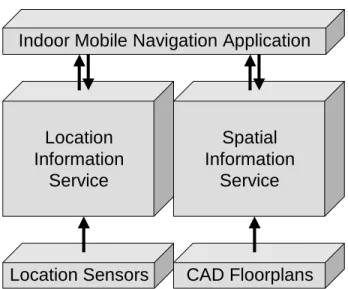
Indoor Mobile Navigation Application Location Sensors Location Information Service Spatial Information Service CAD Floorplans

Figure 1-2: Components required for CricketNav.

to display the locations of nearby resources such as printers and other devices of interest. More importantly, the same resource discovery applications may use the navigation system to locate the positions of various resources and calculate the path length cost relative to the user’s current position. This allows a user to find, for example, the nearest uncongested printer to the user’s current position.

1.2 Design Overview

CricketNav is a mobile navigation application that runs on a handheld computing device connected to a wireless network. CricketNav interacts with two supporting systems to ob-tain the necessary information for navigation (Figure 1-2). The Spatial Information Service provides maps of the physical structure and the spatial layout of the indoor environment. CricketNav uses this information to perform path planning, to determine the direction of the navigation arrow with respect to the user’s current position, and to render a graphical representation of the physical surrounding on the handheld display. The Location Informa-tion Service periodically updates CricketNav with the user’s current posiInforma-tion. CricketNav uses the position updates to anchor the starting point of a path leading to the destination, to prefetch the relevant maps from the spatial information service, to update the current position and direction of the navigation arrow, and to determine when to recalculate a new path for a user who has wandered off the original course.

We use the Cricket location-support system to supply location updates to the appli-cation [18, 19]. The details of the original Cricket system, extensions made to Cricket to support CricketNav, and an evaluation of Cricket’s positioning performance are described in Chapter 2. For the Spatial Information Service, we convert architectural CAD floorplans into a data representation that can be conveniently used for both path planning and ren-dering. The process used for automatic data conversion, and the data structures used for representing spatial information are described in Chapter 3. Chapter 4 describes the design and implementation of CricketNav and Chapter 5 concludes this thesis with a discussion of deployment issues and the current status of CricketNav.

(12)

1.3 Contributions

This thesis makes three main contributions

• Cricket: A modular data processing architecture for the Cricket location system, and

an extensible API for accessing Cricket location information. Implementation and evaluation of a position estimation algorithm for Cricket.

• An automated process of converting architectural CAD floorplans into a spatial data

representation that is useful for a variety of location-aware applications.

• An interactive indoor navigation application that adapts to the quality of information

(13)

Chapter 2

The Cricket Location

Infrastructure

CricketNav requires periodic updates from a location information service to determine the user’s current position, which is then used as the anchor point for selecting an appropriate path and arrow direction for the user to follow. In this chapter, we discuss the location infrastructure requirements for our indoor navigation system and briefly describe some possible location sensing technologies. We then describe the Cricket location system and the software extensions made to it for CricketNav. We conclude this chapter with an experimental evaluation of Cricket’s positioning performance.

2.1 Requirements

There are three requirements for an indoor location support system. The first concerns the types of location information offered by the system. The second concerns its performance in terms of accuracy and latency. The third concerns the practicality of deployment and maintenance of these systems.

2.1.1 Space Location

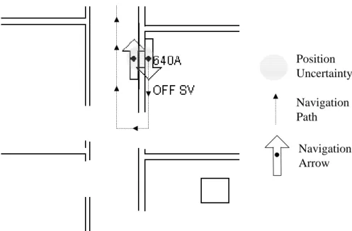
In practice, it is not sufficient to use only coordinate information for navigation. Although there is enough information to match a reported coordinate to a location point in a map, the uncertainty of coordinate estimates sometimes crosses the boundary between two spaces. The error in the reported coordinate may cause the location point to be mapped into a different space, which in turn causes the system to give a navigation direction at the wrong anchor position (see Figure 2-1). The error in the resulting navigation direction is often large because indoor boundaries fundamentally define the shape and the direction of navigation pathways.

Our experience with CricketNav suggests one way of greatly reducing, and sometimes eliminating, this source of error. We rely on the location infrastructure to report the current space in which the user is located. A space is an area defined by some physical or virtual boundary in a floorplan such as a room, a lobby, a section of a large lecture hall, etc. CricketNav uses the reported space information to help keep the location point within the boundary of the current space in which the user is located. For example, a location system may report that the user is inside the office 640A to disambiguate the two possible

(14)

Position Uncertainty Navigation Path Navigation Arrow

Figure 2-1: A person carrying a CricketNav device is in the office 640A so the correct navigation arrow should point downwards. However, small errors in reported coordinate value may cause the navigation arrow to anchor outside the room and point in the wrong direction.

navigation arrows shown in Figure 2-1.

2.1.2 Accuracy and Latency

This section discusses the accuracy and latency requirements of a location system to support CricketNav. For the purpose our discussion, we define location accuracy to be the size of the uncertainty region as illustrated in Figure 2-1. For simplicity, we model the uncertainty

region as a circle, with the center representing the mean reported (x, y) position1 _{under a}

normal distribution of independent samples. The radius of the region is set to two standard deviations of the linear distance error from the mean location. Thus the true location should lie within the uncertainty region in 95% of the time. The update latency is simply defined to be the delay between successive location updates.

CricketNav uses location information to mark the user’s current position on a floor map. Thus, the location system needs to be accurate enough so that CricketNav does not mark the user’s current position in the wrong space. As discussed in the previous section, CricketNav uses space information to reduce this type of error. Hence, it is essential that the location system reports space locations with high accuracy. In particular, the location system should accurately detect opaque space boundaries defined by objects such as walls. However, the reported space do not have to be strictly accurate at open space boundaries, such as those located at a doorway. Whether the reported location lies just inside or outside the open boundary, the navigation direction will be similar.

The reported position should also be accurate enough so that it roughly corresponds to the relative positions in the real setting. For example, if a user is standing to the right of one door, it would be confusing to mark the user’s position indicating that he/she is standing

(15)

to the left of it. In this case, a reasonable position accuracy—in terms of the uncertainty radius—should be between 30 to 50 cm, which is half the width of a typical door.

The final performance requirement is the update latency, which is the delay between successive location updates. Ideally, the update rate should be no less than once in one to two seconds, and the update rate should remain fixed whether the user is standing still or walking. The latter requirement implies that the location system is capable of tracking a user continuously while she is in motion. Some location system tracks a user discontinuously, which means that a location update is given only when the user is stationary. Continuous tracking is very difficult to implement for most location systems because these location systems often requires collecting multiple location measurements from the same location in order to achieve a reasonable accuracy. Therefore, we drop the continuous tracking requirement and assume that the user remains stationary for about five seconds whenever she wants a direction update from CricketNav.

2.1.3 Practicalities

There are a number of practical requirements for deploying an indoor navigation system. First, the indoor environment contains many objects such as computers, monitors, metals, and people that interfere with radio signals and magnetic sensors. Hence, a practical lo-cation sensing system should operate robustly in the presence of such interfering sources. Second, the location sensors of mobile devices must have a compact form factor such that it can easily be integrated with small handheld devices. Third, the location system must be scalable with respect to the number of users currently using the system. Finally, the location sensing infrastructure must minimize deployment and maintenance costs. It is un-desirable to require excessive manual configuration, wiring, and/or frequent battery changes to deploy and maintain the system.

2.2 Existing Systems

Over the past few years, a number of location sensing technologies have emerged to provide location information needed for navigation. Below is a brief description of some of these systems.

2.2.1 GPS

The Global Positioning System uses a network of time-synchronized satellites that period-ically broadcast positioning signals [10]. A mobile GPS sensor receives the signals from four or more satellites simultaneously over orthogonal radio frequency (RF) channels. The positioning signals are coded such that the receiver can infer the offset time between each pair of synchronized signals. Moreover, the orbits of each satellite can be predicted; hence, their positions can be calculated at any given time. From the known position of satellites and three or more offset time values, one can calculate the GPS sensor’s current position by trilateration.

Some specialized GPS receivers have integrated inertial sensors to provide continuous position tracking of mobile objects between GPS positioning updates, and offer positioning accuracies to within a few meters in an open outdoor environment. Unfortunately, GPS does not work well indoors as satellite signals are not strong enough to penetrate building walls, or in many urban areas.

(16)

2.2.2 HiBall Tracker

The HiBall Tracker uses synchronized infrared LEDs and precision optics to determine the user’s position with sub-millimeter accuracy with less than a millisecond latency [23]. It consists of deploying large arrays of hundreds to thousands of LED beacons on ceiling tiles and a sophisticated sensor “ball” that is made up of six tiny infrared sensors and optical lenses. Position and orientation estimations are obtained by sighting the relative angles and positions of the ceiling LEDs. Both the sensor and the LED arrays are centrally synchronized by a computer to control the LED intensity and lighting patterns required to determine the user’s position. The system requires extensive wiring, which makes it expensive and difficult to deploy.

2.2.3 RADAR

RADAR uses a standard 802.11 network adapter to measure signal strength values with respect to the base stations that are within range of the network adapter. Because radio signals are susceptible to multi-path and time-varying interference, it is difficult to find a suitable radio propagation model to estimate the user’s current position. Instead, RADAR proposes the construction of a database that records the signal strength pattern of every location of interest. A system administrator does this manually during system installation. At run time, a server compares the signal strength pattern measured by a receiver and tries to infer its location by finding the closest matching pattern in the database. A drawback of this location approach is that the signal pattern that is recorded statically in the database may greatly differ from the values measured in the dynamic environment, where the signal quality varies with time and the noise level in the environment. Thus, RADAR may not operate robustly in a highly dynamic indoor environment.

2.2.4 Bat

The Bat System consists of transmitters attached to tracked objects and mobiles, and an array of calibrated receivers deployed at known locations on the ceiling. RF and ultrasonic signals are transmitted simultaneously from the transmitters. The receivers measures the lag of the ultrasonic signal to infer its time-of-flight from the mobile transmitter. By multiplying the measured time-of-flight with the speed of sound, one can calculate the distance between a receiver and the mobile transmitter. A different distance estimate is obtained for each of the receivers deployed on the ceiling. The known positions of the receivers and their estimated distance from the mobile transmitter are used to calculate the mobile transmitter’s position. One disadvantage of the Bat System is the expensive wiring infrastructure used to relay information collected at the ceiling receivers to a central computer for processing. Then the processed location information must be relayed back to the user’s handheld device. Since the location updates are transmitted periodically over a wireless network, the handheld pays a significant communication and energy overhead. Also, the Bat architecture does not scale well with the number of objects being located in the system. It places the transmitters at the locatable objects. As the number of locatable object increases, the level of contention among Bat transmitters increases.

Nevertheless, Bat is a pioneering location system that successfully demonstrates the ad-vantages of using ultrasonic-based time-of-flight measurements in the indoor environment. Time-of-flight measurements generally provide more robust distance estimations than tech-niques that rely on signal strength, which are prone to interference by random noises

(17)

gen-erated in the environment. Although ultrasound is susceptible to non-line of sight (NLOS) errors caused by deflection and defraction, these errors can be reduced using various filtra-tion techniques. Finally, the timing circuitry required to measure the time of flight at the speeds of sound is simpler and cheaper than the hardware required for measuring the time difference of GPS satellite signals that travel at the speed of light.

2.3 Cricket

CricketNav uses the Cricket location system as a low cost and practical solution to obtain periodic updates about the mobile user’s current space, position, and orientation. Like Bat, Cricket uses a combination of RF and ultrasonic signals to determine the time-of-flight between a transmitter and a receiver. However, the architecture is fundamentally different from the Bat system. The Bat system places passive receivers in the infrastructure and an active transmitter on the mobile device. In contrast, Cricket deploys active transmitters (beacons) in the ceiling and passive receivers (listeners) on the locatable objects and devices. The main advantages of Cricket’s architecture are scalability, privacy, and ease of de-ployment. Because the mobile listener is passive, the level of channel contention does not increase with respect to the number of locatable objects and devices. Having passive lis-teners on the mobile device also fosters a model that facilitates user privacy; a mobile device can determine its location without having to inject any query messages into the in-frastructure, which makes user tracking harder. Cricket is an ad hoc, distributed system. Beacons can be placed almost arbitrarily with little manual configuration and all compo-nents work autonomously without synchronization or centralized control, which simplifies system deployment.

Cricket beacons are programmable, which enhances the support for location-aware ap-plications. Currently, Cricket beacons are programmed to broadcast a space descriptor and its coordinate over the RF channel during each periodic beacon. Thus, a listener can offer two types of location information. One of these is the listener’s space location, which is a named area defined by some physical or virtual boundary such as a room or a section of a lecture hall. The other is the listener’s position expressed in coordinates defined by the beacon coordinate system. Cricket beacons may also be programmed to include bootstrap-ping information such as the network location of the local navigation map server or resource discovery service.

One subtle, but important, distinction here is that the space information is offered directly by the Cricket location system, in contrast to other techniques that might use a spatial map to map a coordinate estimate to a space location. The space locations reported by the latter systems are not useful because we cannot use them to help correct erroneous coordinate estimates. On the other hand, Cricket offers independent and high quality space information. A Cricket listener infers its space location by finding the space descriptor advertised by the nearest beacon; hence, it directly infers the space location without external information such as a map. Moreover, the space location reported by Cricket is near-perfect at space boundaries that are not penetrable by ultrasound (e.g., a wall). Hence, applications can use Cricket’s space information and a map of a floorplan to test if a reported position estimate is ambiguous (i.e., test if the point lies in the wrong space as in Figure 2-1). If the reported position is indeed ambiguous, applications can use the map information to help them guess a position that is consistent with the reported space. Therefore, by offering accurate space information, Cricket allows applications to

(18)

Beacons on ceiling θ B Compass Sensors Horizontal Plane d1 d2

Figure 2-2: The Cricket Compass measures the angle θ with respect to beacon B. correct ambiguous position estimates, which in turn increases the overall robustness of the location system.

Cricket listeners enhanced with Cricket Compass capabilities can provide orientation information [19]. Multiple ultrasonic sensors are mounted on the enhanced Cricket listener so that when the listener is oriented at an angle with respect to a beacon, the same ultrasonic signal hits each sensor at different times. Assuming that the listener is held relatively flat on the horizontal plane, the timing difference can be translated into an angle θ with respect to the beacon B that transmitted the beacon, as shown in Figure 2-2.

All Cricket beacons run the same distributed, randomized algorithm for avoiding colli-sions among neighboring beacons. Additional interference protection is implemented at the listener for detecting signal collisions and dropping beacon samples that are corrupted by an interfering beacon. Unlike many other existing location-sensing technologies, no part of the Cricket system require central control or explicit synchronization. This property helps keep the Cricket location system simple and robust.

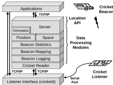
2.4 Software for Cricket: The CricketServer

On their own, the Cricket listeners output raw measured distance samples to a host device via a serial port. The raw data must be processed by a space inference algorithm to determine the current space containing the host device. The raw data must also be processed by a filtering algorithm and a least-square matrix solver to produce sanitized distance and position estimates.

One contribution of this thesis is the design and implementation of the CricketServer, a service program that processes raw Cricket distance measurements from a particular Cricket listener into location information. Instead of implementing its own routines to process raw data, location-aware applications can simply connect to the CricketServer to obtain periodic location updates. The CricketServer normally runs in the handheld device attached to the Cricket listener but it can also run on the network to free up scarce CPU cycles on the handheld. The following sections discusses the CricketServer in detail.

(19)

Cricket Reader Beacon Logging Beacon Mapping Beacon Statistics

Listener Interface (cricketd)

Cricket Listener Cricket Beacon Position TCP/IP Space Orientation Server Applications TCP/IP TCP/IP Data Processing Modules Serial Port Location API

Figure 2-3: Software architecture for CricketServer.

2.4.1 Overview

The CricketServer is composed of a Cricket listener interface called cricketd2, a stack of

data processing modules, and a server that interfaces with location-aware applications. The software architecture for the CricketServer is shown in Figure 2-3.

Whenever a new beacon sample is received, the Cricket listener hardware checks the integrity of the received beacon packet. If not in error, it sends both the beacon and the time-of-flight measurement to cricketd via the serial port. In turn, cricketd pushes this unprocessed beacon via TCP/IP to the data processing stack and to other registered applications soliciting unprocessed data. Hence, applications and data processing modules may run locally on the host machine to which a listener is attached or remotely on a network-reachable server machine.

The data processing modules collect and convert time-of-flight measurements into loca-tion informaloca-tion such as space and posiloca-tion. Each module represents a basic data processing function and the output of each module is pushed to the input queue of the next until the data reaches the server, where location information is dispatched to all registered applica-tions. Intermediate results may be multiplexed to different modules so that common data processing functionalities may be consolidated into one module. For example, the posi-tion and space inference modules may share a common module that filters out deflected time-of-flight measurements.

The modular data processing architecture has a couple of other advantages. For instance, one can experiment with different space inferencing algorithms by simply replacing the space inferencing module. In addition, new modules may be added later without affecting the existing ones. For example, if accelerometers are added to the basic Cricket listeners, new modules may be added to process the acceleration information without affecting the processing done by the existing modules.

(20)

2.5 Data Processing Modules

This section describes the data processing modules shown in Figure 2-3.

2.5.1 Cricket Reader Module

The Cricket Reader Module (CRM) is responsible for fetching raw beacon readings from a variety of beacon sources, which can be a local or remote instance of cricketd, a file containing previously logged beacons, or a simulator that generates beacon readings. Once a beacon reading is obtained from the source, it is parsed and fed into higher level processing modules.

2.5.2 Beacon Mapping Module

During system testing and evaluation, Cricket beacons may be moved frequently into dif-ferent locations. Reprogramming the beacon coordinates may become a hassle. Instead, a Beacon Mapping Module (BMM) may be used to append beacon coordinates to the incom-ing beacon messages. By usincom-ing the BMM, beacons do not advertise its coordinates over RF; thus, energy is saved. The beacon coordinate mapping is conveniently stored in a text file so that the coordinates can be modified easily. The beacon mapping can be downloaded over the network as the user device enters the beacon system.

One caveat about using the BMM is that the beacon coordinates must be kept consistent at all times. If a beacon is moved to a new position, the configuration file must be updated. Currently, the update process needs to be done manually. However, we have ongoing re-search in enhancing Cricket beacons with networking and auto-configuration capabilities so that the BMM configuration files can be updated automatically.

2.5.3 Beacon Logging Module

The Beacon Logging Module (BLM) logs beacon readings that can be replayed later by the Cricket Reader Module. This facility helps to debug modules and study the effects of various beacon filtering and position estimation algorithms. The logging facility also helps to support applications that wish to track the history of all the locations that a user has visited.

2.5.4 Beacon Statistics Module

The Beacon Statistics Module (BSM) collects beacon readings over a sliding time window. Distance measurements that occur within the sliding window are grouped by the source beacons. Various statistics such as the mean, median and mode distances are computed for the samples collected in the sliding window. The resulting beacon statistics are passed on to the Space Inferencing and Position Modules. They are also passed to the Server Module and dispatched to applications that have been registered to receive the beacon statistics information.

Space Inferencing Module

In Cricket, each beacon advertises a space descriptor so that a user device can infer its space location [18]. An example space descriptor is shown below:

(21)

A₀ A1 C B “B” “C” “C” “A₁” “A0” “A1”

“spaceid” - advertisedspaceid

value

- space boundary - beacon

spaceid - space label

Figure 2-4: A Cricket beacon pair is used to demarcate a space boundary. The beacons in a beacon pair are placed at the opposite sides of and at equal distance away from the common boundary that they share. There is a beacon pair that defines a virtual space boundary

between A₀ and A₁. Each beacon advertises the space descriptor of the space in which the

beacon is situated. This figure does not show the full space descriptor advertised by each beacon.

[building=MIT LCS][floor=5][spaceid=06]

We associate the listener’s current space location with the space descriptor advertised by the nearest beacon. In order to support this method of space location, we demarcate every space boundary by placing a pair of beacons at opposite sides of the boundary. In particular, each pair of beacons must be placed at an equal distance away from the boundary as shown in Figure 2-4. Note that a pair of beacons may be used to demarcate virtual space boundaries that do not coincide with a physical space-dividing feature such as a wall.

The Space Inferencing Module (SIM) collects the space descriptors advertised by all the near-by beacons and infers the space in which the listener is situated. The SIM first identifies the nearest beacon by taking the minimum of the mode distances of each beacon heard within the sliding window specified in the Beacon Statistics Module. Once the nearest beacon has been identified, its space descriptor is sent to the Server Module to update the user’s space location.

It is important to note that the size of the sliding window in the Beacon Statistics Module must be large enough so that it can collect at least one distance sample from every beacon within the vicinity to identify the nearest beacon within range. The window size should be at least as large as the maximum beaconing period. The beaconing period depends on the number of beacons that are within range of the listener: the more beacons there are, the longer the listener has to wait before it collects a sample from every beacon. Hence, the window size defines the latency of space location and that latency depends on the average beacon density.

2.5.5 Position Module

The Position Module (PM) implements multilateration to compute the listener’s position

in terms of (x, y, z) coordinates. Let v be the speed of sound, di be the actual distance to

each beacon Bi at known coordinates (xi, yi, zi), and ˆti be the measured time-of-flight to

(22)

Beacons on ceiling B y x z (x_i, y_i, 0) (x, y, z) Cricket Listener’s coordinates

Figure 2-5: The coordinate system used in Cricket; the beacons are configured with their coordinates and disseminate this information on the RF channel.

(x − x_i)2+ (y − y_i)2+ (z − z_i)2= d2_i = (v ˆt_i)2 (2.1)

If the beacons are installed on the same x-y plane (e.g. a ceiling), we can set zi =

0.3 _{Thus, the coordinate system defined by the beacons has a positive z axis that points}

downward inside a room, as shown in Figure 2-5. Consider m beacons installed on the

ceiling, each broadcasting their known coordinates (x_i, y_i, 0). We can eliminate the z2

variable in the distance equations and solve the following linear equation for the unknown listener coordinate P = (x, y, z) if the speed of sound v is known:

A~x = ~b (2.2)

where the matrix A and vectors ~x,~b are given by

A =      2(x1− x0) 2(y1− y0) 2(x₂− x₀) 2(y₂− y₀) ... 2(xm−1− x0) 2(ym−1− y0)     , ~x = " x y # , ~b =        x2 1− x20+ y12− y02− v2( ˆt21− ˆt20) x2 2− x20+ y22− y02− v2( ˆt22− ˆt20) .. . x2_m−1− x2₀+ y_m−12 − y₀2− v2( ˆt2 m−1− ˆt20)        , m ≥ 3

When m = 3, there are exactly two equations and two unknown and A becomes a square matrix. If the determinant of A is non-zero, then Equation (2.2) can be solved to determine unique values for (x, y). Substituting these values into Equation (2.1) then yields a value for z.

When more than three beacons are present (m > 3), we have an over-constrained system.

3_{The results presented here hold as long as z}

(23)

In the presence of time-of-flight measurement errors, there may not be a unique solution

for (x, y). We can still solve for an estimated value (x0_{, y}0_{) by applying the least-squares}

method. For a general system of linear equations, the least-squares method finds a solution

~

x0 _{that minimizes the squared error value δ, where}

δ = (A~x0_{− ~b)(A~}_x0_{− ~b)}T_, _x_~0 ₌ "

x0

y0 #

In some sense, the least-squares approach gives the “best-fit” approximation to the true position (x, y). However, the notion of “best-fit” here is a solution that minimizes δ, which is the squared error expressed in terms of a set of linearized constraints; it does not correspond to a solution that minimizes the physical distance offset between the true and estimated positions. Nevertheless, our experimental results presented in Section 2.6 show that the linearized least-squares solution produces estimates that are reasonably close to the true values.

We note that there is a variant to the position estimation approach described above. Instead of assuming a nominal value for the speed of sound, we can treat it as an unknown

and rearrange the terms in Equation (2.2) to solve for (x, y, z, v2) as discussed in [19]. The

expression for A, x,~b becomes:

A =          2(x1− x0) 2(y1− y0) tˆ21− ˆt20 2(x2− x0) 2(y2− y0) tˆ22− ˆt20 2(x1− x0) 2(y1− y0) tˆ23− ˆt20 .. . 2(xm−1− x0) 2(ym−1− y0) t2m−1ˆ − ˆt20          , ~x =    x y v2   , ~b =       x2 1− x20+ y21− y02 x2 2− x20+ y22− y02 .. . x2 m−1− x20+ ym−12 − y02      , m ≥ 4

This approach solves for v dynamically using the time-of-flight measurements. Since the speed of sound can vary with environmental factors such as temperature, pressure, and humidity [7], this approach might improve the positioning accuracy when the location system operates in varying environmental conditions. When the listener collects distance samples from five or more beacons (m ≥ 5), we can further improve the position estimation

accuracy by applying least-squares to find a “best-fit” solution for (x, y, z, v2_).

We can still apply other heuristics to use the extra beacon distance measurements when-ever they are available. For example, we can choose the three “best” beacon distance es-timates out of the set of beacons heard in the sliding window (from BSM) to estimate the listener’s position. Alternatively, we can compute a position estimate from all possible combinations of three beacon distances, and then average all the results to obtain the final position estimate [5]. In practice, extra beacons may not always be within range of the listener as the number of redundant beacons deployed may be minimized to reduce cost. The best algorithms should adapt to the information that is available.

(24)

latency, which can increase as a Cricket listener tries to collect distance samples from more beacons. In our current implementation, we impose a latency bound by specifying a sliding sampling window of five seconds in the BSM. Then we apply the following heuristic based on our experimental results described in Section 2.6: If distance samples are collected from fewer than five beacons within the sliding window, we assume a nominal value for the speed

of sound, and apply least-squares to solve for (x0_{, y}0_{, z}0_{). When the listener collects distance}

samples from more than or equal to five beacons within the sampling window, we treat the speed of sound as unknown and apply least-squares on all the available constraints to solve for (x0_{, y}0_{, z}0_{, v}02_{). This heuristic improves the accuracy of our position estimates while}

keeping the latency acceptably low.

Besides collecting samples from multiple beacons, a listener may collect multiple distance samples from the same beacon within a sampling window. In this case, the BSM helps refine the distance estimate to a beacon by taking the mode of the distances sampled for that beacon. Taking the mode distance value effectively filters out the reflected time-of-flight measurements [18, 20].

Finally, the multilateration technique discussed above assumes that the listener is sta-tionary while it is collecting distance samples. More specifically, Equation (2.2) assumes

that the ˆtimeasurements are consistent with a given listener coordinate so that the equation

can be solved simultaneously [24]. However, when the listener is mobile, as in our naviga-tion applicanaviga-tion, the distance samples collected from each beacon are correlated with the listener’s velocity. As the user moves, successive distance samples will be collected at a dif-ferent location; thus, the simultaneity assumption in Equation (2.2) is violated. In Cricket, the time lag for collecting samples from three different beacons takes at least 0.5 to 1 second. Assuming the mobile user travels at 1 m/s, the distance estimates can vary between 0.5 to 1 meter. Thus, we cannot simply ignore how mobility affects position estimation.

To continuously track the position of a mobile user, we need a more sophisticated posi-tioning technique such as integrating inertial sensors to the Cricket listener and/or adopt-ing the Sadopt-ingle-Constraint-At-A-Time (SCAAT) trackadopt-ing algorithm presented in [23, 24]. The original SCAAT algorithm was developed for the HiBall tracking system and must be adapted to Cricket. In this thesis, we implement the stationary positioning technique described above and assume that the listener stays stationary for a few seconds before its position can be reported. Ideally, the listener should remain stationary until all the stale distance samples is flushed from the sliding window in the BSM.

Orientation Module

The Orientation Module (OM) processes data from a Cricket Compass and outputs ori-entation information in terms of θ and B, which are the relative horizontal angle and the reference beacon shown in Figure 2-2. Currently, we have not implemented the OM module but the algorithm for estimating θ can be easily implemented [19]. The Cricket Compass

finds θ by measuring the absolute differential distance |d1− d2| with respect to a reference

beacon B. The algorithm for estimating θ involves computing the mode of a sequence of differential distance samples reported by the Cricket Compass, and performing a table lookup for translating the difference into an angle value. The final step of the algorithm uses the output of the Position Module to calculate a number used to scale the final result for θ.

The CricketServer is not limited to process orientation measurements from a Cricket Compass. We can just as easily implement and load an orientation module that processes

(25)

Beacon Name (x, y, z) 506A 427, 183, 0 506B 0, 122, 0 506C 244, 244, 0 506D 61, 61, 0 510A 61, 488, 0 510B 0, 305, 0 510D 427, 305, 0 600LL 366, 61, 0 600LR 244, 366, 0 613B 366, 427, 0 615 122, 366, 0 617 183, 0, 0

Table 2.1: Experimental setup: Beacon coordinates (in cm)

data from a digital magnetic compass, and report θ with respect to the magnetic north pole.

Server Module

The Server Module (SM) implements the CricketServer 1.0 protocol to access various lo-cation information produced by the data processing modules. The protocol uses a self-describing format, which makes it extensible. It uses ASCII, which eases the debugging and parsing process during application development. The SM transfers location information over the TCP/IP protocol. Thus applications may fetch processed location information from a specific Cricket listener over the network. The complete specification of the CricketServer 1.0 protocol is in Appendix A.

2.6 Cricket’s Positioning Performance

We conducted an experiment to evaluate the positioning performance of the Cricket location system. In our setup, we placed twelve Cricket beacons on the ceiling of an open lounge area as illustrated in Figure 2-6. To prevent degenerate cases that cause det(A) = 0, we ensured that no three beacons are aligned on a straight line and that no four beacons lie on the same circle. The beacons were configured with the coordinates shown in Table 2.1. We placed a Cricket listener at coordinate (122cm, 254cm, 183cm) and collected over 20000 distance samples from the twelve beacons in about an hour. For each distance sample, we recorded the time stamp and the source beacon that generated the distance sample. The listener remained stationary for the duration of the experiment.

2.6.1 Sample Distribution

Figure 2-7 plots the distribution of logged samples. The plot shows an uneven distribution of samples collected from the different beacons. In particular, the listener received very few successful transmissions from beacon 510D over the one hour period. We do not know the

(26)

Cricket Listener

Figure 2-6: Experimental setup: Beacon positions in the ceiling of an open lounge area

600 800 1000 1200 1400 1600 1800 2000 2200 506A 506B 506C 506D 510A 510B 510D 600LL600LR 613B 615 617

Number of collected sample

Beacon ID

(27)

exact cause of this behavior but we suspect that beacon 510D may have a faulty antenna that is emitting an unusual RF radiation pattern. When the strength of the RF radiation from a faulty beacon is not evenly distributed in free space, the neighboring beacons may not detect its transmission. Thus, the neighboring beacons incorrectly assume that the channel is clear for transmission. Instead of staying silent to avoid a collision, the neighboring beacons attempt to transmit while the faulty beacon is transmitting. Consequently, the listener receives fewer successful samples from the faulty beacon.

2.6.2 2D Positioning Accuracy

Recall from Section 2.5.5 that the position estimates depend on the distance estimates to the individual beacons. Thus, it is intuitive that if we improve the accuracy of the individual distance estimates, we would improve the accuracy of the position estimates. One way to improve accuracy of distance estimates is to collect multiple distance samples from each beacon and then take either the mean or the mode of these values. Alternatively, we can collect distance samples from a large number of beacons, which increases the number of constraints in the linear system of Equation (2.2). Denote k to be the sample frequency, which we define to be the number of samples collected from each beacon. Also, we denote m to be the beacon multiplicity or the number of distinct beacons from which distance estimates are collected, which is equivalent to the number of constraints in the linear system. We examine how the positioning accuracy varies with k and m from our experimental values.

Because 2D position estimates in the xy plane are sufficient for a large number of applications such as CricketNav, we analyze the 2D positioning accuracy. For our analysis, we define the position estimation error, ², to be the linear distance between the listener’s

true coordinate (x, y) and the estimated coordinate (x0_{, y}0_{) produced by the least-square}

algorithm:

² =

q

(x − x0₎2_{+ (y − y}0₎2

Thus, we ignore the z component in our accuracy analyses. Methodology

We obtain our experimental results by randomly choosing distance samples from our data log and process the selected set of samples to obtain a least-squares position estimate. More precisely, we first group the collected data into twelve sample arrays, each containing distance samples from a single beacon. For each position estimation trial, we randomly pick

m beacon arrays, and from each array, we randomly pick k samples. To obtain distance

estimates to each beacon, we take either the mode (denoted as “MODE”) or the mean (denoted as “MEAN”) of the k samples chosen from each beacon. For MODE, the distance estimate is set to the average of all modal values when there is more than one distance value occurring with same maximal frequency. Using either MODE or MEAN, we compute a distance estimate for each of the m beacons. Then we plug the distance estimates into a squares solver to obtain a position estimate. As mentioned in Section ??, the least-squares solver can find a position estimate by treating the speed of sound as a known value or an unknown variable. We compare the position estimates for both and denote them as KNOWN and UNKNOWN respectively. From each position estimate we get, we compute

(28)

500 trials. We take the average position error, ², over these 500 trials as our final result for the experiment.

Occasionally, we obtain a set of distance estimates that yield imaginary results, where

either z2 _{< 0 or v}2 _{< 0. We ignore these values in our reported results. We note, however,}

that no more than 25% of the trials in all our experiments gave imaginary numbers for the range of k and m values we have chosen.

The nominal value we used for the speed of sound, v, is 345m/s, which is the expected

value at 68◦_{F [7]. Unless stated otherwise, the speed of sound is treated as a known value}

when we compute a least-squares estimate.

Our experiment method closely emulates how the CricketServer collects and processes beacon samples from the Cricket listener. In particular, we randomly choose a subset of

m beacons out of the twelve beacons. The geometry of beacon placement is known to

affect positioning accuracy in other location systems [14]. We do not yet understand how the beacon placement geometry in our setup affects the results in our experiment. But by selecting m beacons randomly in every trial, we obtain position estimates from different beacon configurations. Thus, this strategy minimizes the bias that might arise from using samples from only a fixed set of m beacons in a fix geometric configuration.

Results and Analysis

Figure 2-8 plots ² as a function of k using MEAN distance estimates. The different curves represent the results obtained by varying the beacon multiplicity, m. For example, the curve MEAN4-KNOWN shows the results obtained by collecting samples from four beacons (m = 4). The figure shows that the positioning accuracy do not improve as the sample frequency, k, increases. To explain why the accuracy does not improve, we note that there are occasional spikes in the distance measurements caused by reflected ultrasonic signal in the environment. Such measurements skews the average of the measured distance samples. Also, the likelihood of sampling a reflected distance reading increases with k. Thus, the average ² actually increased slightly with k. However, we note that the positioning error decreases with increasing m. This result is expected because increasing the beacon multiplicity is equivalent to increasing the number of constraints in the linear system to improve the fitting of the position estimate.

Figure 2-9 plots ² as a function of k using MODE distance estimates. This figure shows that ² decreases with k. When a large number of samples are collected from each beacon (k > 5), MODE effectively filters out the reflected distance readings. However, when few samples are collected (i.e., k ≤ 5), it is difficult to collect enough consistent samples to benefit from MODE. Essentially, the MODE distance estimation becomes a MEAN distance estimation for small values of k. Some evidence of this is shown by comparing the similar values of ² measured at k = 1, 2 in Figures 2-8 and 2-9.

Also from Figure 2-9, we note that the results for MODE3-KNOWN represents a non-least-square solution because the beacon multiplicity is three, which means that there are exactly three equations and three unknowns. In this case, MODE3-KNOWN does not benefit from the least-squares fitting effect that would be induced by an over-constrained system. Nevertheless, the average error from MODE3-KNOWN is not too much larger than the errors from the other least-square position estimates.

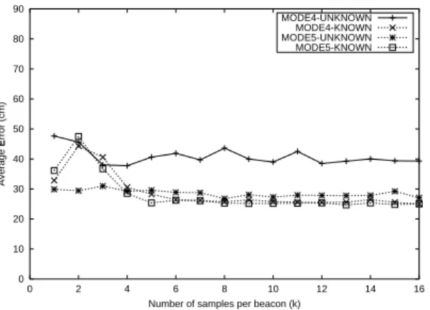
Figures 2-10 and 2-11 compares the results obtained from a linear system that solves the speed of sound, v, as an unknown (UNKNOWN) versus one that assumes a nominal value for the speed of sound (KNOWN). The MODE4-UNKNOWN curves in both figures

(29)

0 10 20 30 40 50 60 70 80 90 0 2 4 6 8 10 12 14 16 Average Error (cm)

Number of samples per beacon (k) MEAN3-KNOWN MEAN4-KNOWN MEAN5-KNOWN MEAN6-KNOWN MEAN7-KNOWN MEAN8-KNOWN

Figure 2-8: Position Error (cm) vs. k us-ing MEAN distance estimates. The speed of sound is assumed known when calculating the position estimate.

0 10 20 30 40 50 60 70 80 90 0 2 4 6 8 10 12 14 16 Average Error (cm)

Number of samples per beacon (k)

MODE3-KNOWN MODE4-KNOWN MODE5-KNOWN MODE6-KNOWN MODE7-KNOWN MODE8-KNOWN

Figure 2-9: Position Error (cm) vs. k us-ing MODE distance estimates. The speed of sound is assumed known when calculat-ing the position estimate.

0 10 20 30 40 50 60 70 80 90 0 2 4 6 8 10 12 14 16 Average Error (cm)

Number of samples per beacon (k) MODE4-UNKNOWN

MODE4-KNOWN MODE5-UNKNOWN MODE5-KNOWN

Figure 2-10: Position Error (cm) vs. k us-ing MODE distance estimates and varyus-ing

m between 4 and 5. The curves labeled

UN-KNOWN (UN-KNOWN) represent the results obtained from a linear system that assumes an unknown (known) speed of sound.

0 10 20 30 40 50 60 70 80 90 0 2 4 6 8 10 12 14 16 Stddev Error (cm)

Number of samples per beacon (k) MODE4-UNKNOWN-STDDEV

MODE4-KNOWN-STDDEV MODE5-UNKNOWN-STDDEV MODE5-KNOWN-STDDEV

Figure 2-11: Standard deviations of the re-sults reported in Figure2-10.

(30)

0 10 20 30 40 50 60 70 80 90 3 4 5 6 7 8 9 10 11 12 Average Error (cm)

Number of sampled beacons (m)

UNKNOWN KNOWN

Figure 2-12: Position Error (cm) vs. m for

k = 1. 0 10 20 30 40 50 60 70 80 90 3 4 5 6 7 8 9 10 11 12

Standard Deviation Error (cm)

Number of sampled beacons (m)

UNKNOWN-STDDEV KNOWN-STDDEV

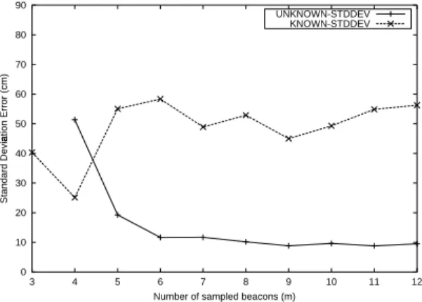
Figure 2-13: Standard deviations of the re-sults reported in Figure2-12.

respectively plot the values for the average error, ², and the standard deviation of the position error over 500 trials, σ(²). The results of these curves are obtained by treating v as an unknown. In this case, there are exactly four constraints and four unknowns in the linear system. Thus, there is no redundancy in the system to induce a least-squares-fitted solution. Indeed, the positioning estimates are poor for MODE4-UNKNOWN when compared to MODE4-KNOWN, which has one extra constraint. However, the results are not always poor when we solve v as an unknown. For example, all the MODE5-UNKNOWN curves have generally lower estimation errors and standard deviations than MODE5-KNOWN. Although KNOWN has one more constraint in the linear system than MODE5-UNKNOWN, both systems have a beacon multiplicity that is greater than the number of unknowns in the linear system. Hence, both MODE5-KNOWN and MODE5-UNKNOWN are over-constrained and both schemes induce a least-squares-fitted position estimate. One fundamental difference between the two schemes is that MODE5-KNOWN finds a best-fit estimate in the x, y space whereas MODE5-UNKNOWN finds a best-fit estimate in the

x, y, v2 _{space. We do not understand the theoretical implications of this difference but}

our experimental results show that for k ≤ 5, the MODE5-UNKNOWN scheme performs better, while it performs similarly to MODE5-KNOWN when k > 5. Although we do not have an explanation for these results, the two figures suggest that the least-squares method is a significant factor in minimizing ², especially when k is large. This relationship holds in all our experiments with m ≥ 5.

We paid particular attention to the results at k = 1 because the previously discussed figures 2-10 and 2-11 respectively show that the positioning error and standard deviation decreases as m increases. To verify if the trend holds, we plot ² and σ(²) as a function of m at k = 1 in Figures 2-12 and 2-13 respectively. The curves labeled KNOWN (UNKNOWN) represents the results obtained from a linear system that assumes the speed of sound is known (unknown). The errors and standard deviations of the UNKNOWN curves decreases with increasing m but an opposite trend occurs for KNOWN. Currently, we do not have an explanation for this. However, our results suggest an interesting way to optimize the beacon placement strategy to improve the accuracy of estimating position: We should increase the

beacon density4 _{such that the listener can hear from five or more beacons from any location.}

(31)

0 0.2 0.4 0.6 0.8 1 1.2 0 10 20 30 40 50 60 CDF Ratio Error (cm) MODE3-KNOWN MODE4-KNOWN

Figure 2-14: Cumulative error distribution for k = 1 and m = 3, 4. Speed of sound is assumed known. The horizontal line repre-sents the 95% cumulative error.

0 0.2 0.4 0.6 0.8 1 1.2 0 10 20 30 40 50 60 CDF Ratio Error (cm) MODE5-UNKNOWN MODE6-UNKNOWN MODE7-UNKNOWN MODE8-UNKNOWN MODE9-UNKNOWN MODE10-UNKNOWN MODE11-UNKNOWN MODE12-UNKNOWN

Figure 2-15: Cumulative error distribution for k = 1 and 5 ≤ m ≤ 12. Speed of sound is assumed unknown. The horizontal line represents the 95% cumulative error. Assume that the BSM uses a small sliding window to collect only one sample from each beacon (i.e., assume k = 1), we now analyze if our positioning algorithm yields the required accuracy as mentioned in Section 2.1.2. To minimize positioning error for all m, our least-squares positioning algorithm crosses-over between UNKNOWN and KNOWN depending on the number of distinct beacons sampled in the BSM’s sliding window. Figure 2-12 shows that the cross-over point is at m = 5. Thus, to test if our positioning algorithm meets CricketNav’s accuracy requirements, we plot the cumulative distribution function (CDF) of the positioning error in two figures. Figure 2-14 plots the CDF for m ≤ 4, and the speed of sound is KNOWN, and Figure 2-15 plots the CDF for m > 4, and the speed of sound is UNKNOWN. The highest error value intersected by the 95% horizontal line in both figures is no greater than 30cm. Hence, we conclude that our positioning algorithm meets CricketNav’s accuracy requirement; our positioning algorithm produces results that have less than 50cm position error 95% of the time.

We summarize the results of our positioning accuracy analysis:

• A MODE distance estimation produces more accurate position estimates than MEAN. • MODE does not begin to take effect until k >= 5.

• The least-squares method described in Section 2.5.5 effectively reduces positioning

errors.

• For k < 5 and m ≥ 5, it is better to assume speed of sound is unknown. Otherwise,

it is better to assume speed of sound is known.

• For k = 1, Cricket is accurate to within 30cm, 95% of the time.

(32)

2.6.3 Latency

From the previous section, we learn that the positioning accuracy varies with the number of samples collected per beacon, k, and the number of distinct beacons sampled, m. Con-ceivably, we could specify the values of these parameters in the CricketServer to obtain the desired positioning accuracy. Such a feature would be useful if applications require strict guarantees on positioning accuracy. However, the cost of guaranteeing accuracy is latency, which we define here as the time it takes to collect enough samples to compute a position estimate with a certain accuracy. As in the previous section, we parameterize accuracy by

k and m. Thus, for our experiments, we define latency to be the time it takes to collect k

distance samples from m different beacons. Since CricketNav have requirements for both positioning accuracy and latency, it is interesting to study how latency varies with k and

m. The following sections describes our experimental results on latency.

Methodology

We wish to design an experimental methodology that closely resembles a typical situation that would be faced by the CricketNav application. In a typical situation, Cricket beacons are deployed throughout the building. A Cricket listener receives a successful sample only if it is within range of a beacon’s ultrasonic and radio transmissions. This requirement has an implicit effect on latency. For example, a listener may not receive a successful sample from a beacon that is situated in a neighboring room; while the radio signal can pass through the wall standing between the beacon and the listener, the ultrasound cannot. Thus, if there are a large number of interfering beacons in the neighboring rooms, a large number of received radio transmissions will be dropped by the listener, which then increases the delay to collect a distance sample from every beacon in the same room.

In our experiments, we assume that the Cricket listener is within radio range of twelve beacons. This is a realistic assumption if the beacon density is low and the radio range is short. Next, we assume that the Cricket listener is within ultrasonic range of m beacons. Thus, as we vary m, we model that there are 12 − m interfering beacons.

We measure the average latency by sampling our data log. Recall that each distance sample in our log were recorded with a time stamp and that the log entries are sorted in time order. Before each sampling trial, we randomly pick a set of m beacons. To measure the average latency, we randomly choose a starting time in the log file and scan forward until we have read at least k samples each from the m selected beacons. The scan wraps around to the first entry if it continues through the end of the log. After the scan stops, the time difference between the time stamps at the starting and stopping points of the scan becomes the latency result for one trial. The final latency result for an experiment with specific values for k and m is computed by averaging the latency over 500 trials.

Results and Analysis

Figure 2-16 shows the mean and median latency of collecting one sample from varying number of different beacons. The latency stays at around 3.25s for different values of m. The latency does not depend on m because the scan stops only after it collects at least one sample from a randomly-predetermined subset of m beacons. Note that the average delay for collecting a sample from a specific beacon is half of the beacon’s average beaconing period. On average, every beacon gets to transmit once within a beaconing period. Thus, the average waiting time is the same whether we collect one sample each from a few beacons