HAL Id: hal-02291224
https://hal-essec.archives-ouvertes.fr/hal-02291224
Preprint submitted on 18 Sep 2019HAL is a multi-disciplinary open access archive for the deposit and dissemination of sci-entific research documents, whether they are pub-lished or not. The documents may come from teaching and research institutions in France or abroad, or from public or private research centers.
L’archive ouverte pluridisciplinaire HAL, est destinée au dépôt et à la diffusion de documents scientifiques de niveau recherche, publiés ou non, émanant des établissements d’enseignement et de recherche français ou étrangers, des laboratoires publics ou privés.
How Serious is the Measurement-Error Problem in a
Popular Risk-Aversion Task?
Fabien Perez, Guillaume Hollard, Radu Vranceanu, Delphine Dubart
To cite this version:
Fabien Perez, Guillaume Hollard, Radu Vranceanu, Delphine Dubart. How Serious is the Measurement-Error Problem in a Popular Risk-Aversion Task?. 2019. �hal-02291224�
How Serious is the
Measurement-Error Problem in
a Popular Risk-Aversion Task?
FABIEN PEREZ, GUILLAUME HOLLARD, RADU VRANCEANU, DELPHINE DUBART
ESSEC RESEARCH CENTER
WORKING PAPER 1911
SEPTEMBER, 2019
How Serious is the Measurement-Error Problem in a Popular
Risk-Aversion Task?
∗Fabien Perez†, Guillaume Hollard ‡, Radu Vranceanu §
Delphine Dubart ¶
September 17, 2019
Abstract
This paper uses the test/retest data from the Holt and Laury (2002) experiment to provide estimates of the measurement error in this popular risk-aversion task. Maximum-likelihood estimation suggests that the variance of the measurement error is approxi-mately equal to the variance of the number of safe choices. Simulations confirm that the coefficient on the risk measure in univariate OLS regressions is approximately half of its true value. Unlike measurement error, the discrete transformation of continuous risk-aversion is not a major issue. We discuss the merits of a number of different solutions: increasing the number of observations, IV and the ORIV method developed by Gillen et al. (2019).
Keywords: Experiments; Measurement error; Risk-aversion, Test/retest; ORIV. JEL Classification: C18; C26; C91; D81.
∗The authors are grateful to Olivier Armantier, Gwen-Jiro Clochard, Paolo Crosetto, Jules Depersin,
Anto-nio Filippin, Lucas Girard, Yannick Guyonvarch, Xavier d’Haultfoeuille, Nicolas Jacquemet and participants at the 10th International Conference of the ASFEE 2019 in Toulouse and the ESA European meeting 2019 in Dijon for their suggestions and remarks that helped to improve this work.
†CREST, INSEE - 5 Avenue Le Chatelier, 91120 Palaiseau. E-mail: [email protected].
‡CREST, Ecole Polytechnique, CNRS - 5 Avenue Le Chatelier, 91120 Palaiseau. E-mail:
§ESSEC Business School and THEMA, 1 Avenue Bernard Hirsch, 95021 Cergy. E-mail:
1.
Introduction
Economists explain individual heterogeneity in observed behavior by appealing to a num-ber of key individual characteristics, such as risk attitudes or time preferences. A common research practice is to elicit this kind of individual characteristic via an elementary task, and then use the resulting value as an explanatory variable in subsequent regressions. One example is the use of an elicitation method to measure risk attitudes, for example that pro-posed by Holt and Laury (2002), and then including the outcome from the task in some OLS regressions.
The potential issue here comes from the considerable within-individual variability in these elicited measures. For example, the correlations between different measures of risk attitudes for the same individual are typically small, even when the same task is repeated within a short period of time (see, for instance, the discussion and references in Bardsley et al. (2010)). From an econometric perspective, within-individual variability can be interpreted as mea-surement error, which has well-known negative consequences: in OLS regressions, the coeffi-cient on the explanatory variable measured with error is attenuated, and other variables that are actually not significant in multivariate regressions may wrongly be estimated to be so, as measurement error in one explanatory variable renders all of the estimates inconsistent.
Another difficulty comes from the fact that popular elicitation methods yield a discrete approximation of a continuous variable (e.g. risk-aversion or the discount rate). Round-ing or truncatRound-ing elicited measures will mechanically produce some imprecision. Last, esti-mated risk-aversion often comes from laboratory experiments with relatively small samples (e.g. N=100 or 200). Many experimental-economics analyses then use small samples, with variables that are plagued by measurement error arising from intra-subject variability and rounding issues.
So far, little is known about the magnitude of this measurement error and rounding: What is the degree of attenuation of the coefficients in OLS regressions? How often will significant coefficients actually appear to be insignificant?
In this paper, we use test/retest information to gauge the size of the measurement error in the extremely popular Holt and Laury (2002) (HL) task to measure risk-aversion.1 We here appeal to the relevant original information in Holt and Laury (2002), as they implemented a “return to baseline” task using the same group of participants in a standard test/retest 1In a relatively short period of time, this task has become the most popular risk-aversion elicitation method
in experimental economics, as mentioned for instance in Zhou and Hey (2018), Charness et al. (2019), Attanasi et al. (2018), Crosetto and Filippin (2016). Google Scholar, accessed on 28.08.19, indicates 5400 citations for this paper.
design. We can therefore compare the choices made by the same individual in the same task, repeated within a short period of time (in the same experimental session). As a robustness check, we carried out a test/retest of the HL task at the ESSEC Experimental Lab in 2019 (see Appendix A).
Our analysis proceeds in three steps. (1) we carry out maximum-likelihood (ML) joint estimations of the variance of the measurement error, as well as of the mean and variance of the variable of interest (the number of safe choices in the Holt-Laury task; see the next section for details). (2) We simulate a linear stochastic model and carry out a large num-ber of univariate OLS regressions. We also vary the sample sizes (with N=100 being the benchmark). This allows us to assess the respective impact of the measurement error and rounding on the variance and significance of the estimated coefficient. (3) Finally, we use the simulations to analyze and compare possible solutions to the measurement-error problem, such as increasing the number of observations, using IV estimators or the Obviously Related Instrumental Variables (ORIV) method developed by Gillen et al. (2019).
Two relevant contributions address the issue of measurement error in experimental data. Gillen et al. (2019) replicate three classic experiments using an original data set (the Caltech cohort survey), and show that the results can change dramatically when the measurement error is correctly accounted for. Our analysis here addresses two important elements not considered there: the impact of the sample size (in particular the small sample sizes typical of laboratory experiments) and the rounding issue arising from the use of a discrete measure of a continuous variable. Engel and Kirchakamp (2019) adopt an alternative method to estimate the measurement error in the HL task. Their focus is on inconsistent answers,2
and they aim to estimate an individual-specific error term (while we here assume that the error terms are independent between tasks, and are drawn from the same distribution for all individuals). In contrast, we use test/retest data to evaluate the size of the measurement error. Test/retest is a simpler way of evaluating the importance of measurement error, and can be applied even when the number of inconsistent choices is small.
We find that:
(1) Assuming normal distributions, the maximum-likelihood (ML) estimated variance of the measurement error is close to 1, similar to the variance of the latent risk-aversion variable. In theory, the attenuation factor is close to 0.5, regardless of the size of the sample. Our subsequent simulations indeed indicate that the typical amount of noise in the HL task 2Jacobson and Petrie (2009) record a large number of such mistakes in a different experiment, and argue
will roughly divide the coefficient of interest by 2.
(2) Our simulations also show that in this task the discrete transformation of the variable of interest (i.e. rounding) does not much affect the attenuation bias, and only marginally affects the variance of the estimators. By way of contrast, the measurement error arising from within-subject variability is responsible for much of the effect on the estimated coefficient.
(3) Increasing the sample size does not alleviate the attenuation bias, but does increase the significance of the estimated coefficient. Going up to N = 1000 suffices for the coefficient to become significant almost 100% of the time, while smaller sample sizes (e.g.N = 100 or
N = 200) produce a large proportion of insignificant coefficients.
(4) As expected, the ORIV method almost completely removes the bias, although ORIV estimates have larger variances than the true OLS estimates. ORIV may not suffice to solve the significance issue resulting from measurement error for small samples.
(5) Using ORIV and increasing the sample size are powerful solutions to address the estimation biases induced by measurement error in the Holt and Laury task (and probably other tasks as well).
The remainder of the paper is organized as follows. The next section briefly describes the HL task and the data. Section 3 provides ML estimates for the variance of the measurement error, and the mean and variance of the variable of interest. Section 4 uses these parameters to simulate a linear stochastic model, and then carries out 100000 regressions under different assumptions about the properties of the explanatory variable. The last section concludes.
2.
The Holt and Laury (2002) task: A primer
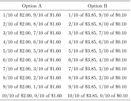
The Holt and Laury (2002) (HL) risk-aversion elicitation task consists in choosing between a ”safe” (small-spread) lottery x
10.2$ + (1−
x
10).1.6$ and a ”risky” (wide-spread) lottery
x
10.3.85$ + (1−
x
Table 1: The Holt and Laury (2002) risk-aversion elicitation task Option A Option B 1/10 of $2.00, 9/10 of $1.60 1/10 of $3.85, 9/10 of $0.10 2/10 of $2.00, 8/10 of $1.60 2/10 of $3.85, 8/10 of $0.10 3/10 of $2.00, 7/10 of $1.60 3/10 of $3.85, 7/10 of $0.10 4/10 of $2.00, 6/10 of $1.60 4/10 of $3.85, 6/10 of $0.10 5/10 of $2.00, 5/10 of $1.60 5/10 of $3.85, 5/10 of $0.10 6/10 of $2.00, 4/10 of $1.60 6/10 of $3.85, 4/10 of $0.10 7/10 of $2.00, 3/10 of $1.60 7/10 of $3.85, 3/10 of $0.10 8/10 of $2.00, 2/10 of $1.60 8/10 of $3.85, 2/10 of $0.10 9/10 of $2.00, 1/10 of $1.60 9/10 of $3.85, 1/10 of $0.10 10/10 of $2.00, 0/10 of $1.60 10/10 of $3.85, 0/10 of $0.10
The data set comes from the initial article by Holt and Laury (2002), who elicited the risk measure for their main treatment (Table 1) twice: once at the beginning of the experimental session and once at the end, after having subjects perform variants of the same task with higher stakes. Their sample included a total of 175 subjects from three US Universities; half were undergraduate students, one third MBA students and the rest business-faculty members.3
Assuming that subjects maximize their expected utility,4 and that their utility function
is twice-differentiable, the value x∗(a continuous variable) for which the subject is indifferent between the safe and the risky lottery is strictly increasing in the coefficient of risk-aversion.
x∗ is thus a valid variable to describe risk preferences, and is our variable of interest. Subjects generally start by choosing the safe option when x = 1 and shift to the risky option for a larger x, more precisely for ⌊x∗⌋ + 1. The number of times the safe option chosen is therefore ⌊x∗⌋. This discrete variable is the standard measure of risk-aversion recommended by Holt and Laury (2002).5 Using a discrete transformation to approximate
a continuous variable introduces some imprecision.
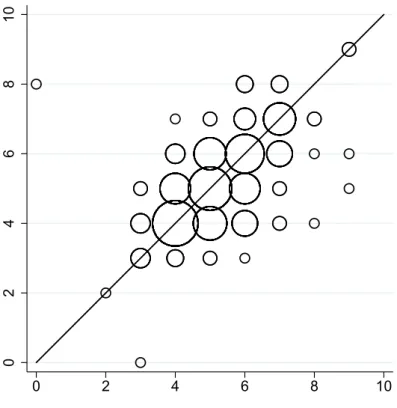
In the scatter diagram in Figure 1, the horizontal axis represents the number of times an individual chose the safe option in the first test, and the vertical axis the same number 3We manually transcribed the data provided at the address http://www.people.virginia.edu
/ cah2k/highdata.pdf.
4The debates around this standard decision model are beyond the scope of the current paper; see
O’Donoghue and Somerville (2018) for a recent discussion.
in the last (retest) test at the end of the session. The size of the circles reflects the number of individuals making a given choice. The dispersion of the circles suggests that noise other than discretization affects the risk-aversion measures. The observed variables with noise and discrete transformation can be written as: x1 =⌊x∗+ ϵ1⌋ and x2 =⌊x∗+ ϵ2⌋, where ϵ1 and
ϵ2 are the noise or measurement errors.
0 2 4 6 8 10 0 2 4 6 8 10
Figure 1: Scatter plot of the number of safe choices in the two repetitions of HL 2002
Finally, as in all MPL tasks, it is not uncommon that some ”inconsistent” subjects switch back from the risky to the safe option. Engel and Kirchakamp (2019) use the information included in these multiple switches to obtain information about the noise. We will follow an alternative path for three reasons. First, the number of multiple switches is only small in the datasets we use (under 10% in the original HL experiment and under 5% in our ESSEC replication). Second, most subjects seem to consider the whole task as one unique choice, choosing the row from which they want to switch to the risky option, and not as a multiple-choice task (Hey et al. (2009)). Third, the two repetitions of the task provide us with enough information to determine the lower bound of the measurement error in this risk-aversion elicitation task.
3.
Estimating the variance of the measurement error
Maximum-Likelihood Assumptions
We wish to estimate the mean and variance of our variable of interest x* and the variance of the measurement error ϵi using standard maximum-likelihood procedures. To do so we use the following notation and simplifying assumptions:
• Variable of interest x∗ ∼ N (m, σx2) truncated over [0,10] (with a density function of
f).
• Measurement error for observation i ∈ {1, 2}, ϵi ∼ N (0, σϵ2)6 (with a distribution
function of Φ).
• ϵ1, ϵ2 and x∗ are all independent of each other.
• We observe x1=⌊x∗+ ϵ1⌋ and x2=⌊x∗+ ϵ2⌋7.
• The unknown parameters are θ ={m, σx, σϵ} .
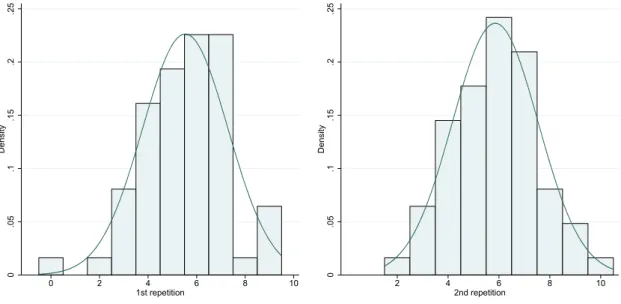
Figure 2 presents the number of safe choices in the test and retest conditions in Holt and Laury (2002). Their shapes suggest that normality is a plausible assumption.
0 .1 .2 .3 Density 0 2 4 6 8 10 1st repetition 0 .1 .2 .3 Density 0 2 4 6 8 10 2nd repetition
Figure 2: Number of safe choices in the two repetitions of HL 2002 6We could assume that ϵ
1 and ϵ2are drawn from normal distributions with different variances.
7In extreme cases we can have x∗+ ϵ < 0 (resp x∗+ ϵ≥ 11): in this case we observe x = 0 (resp x = 10)
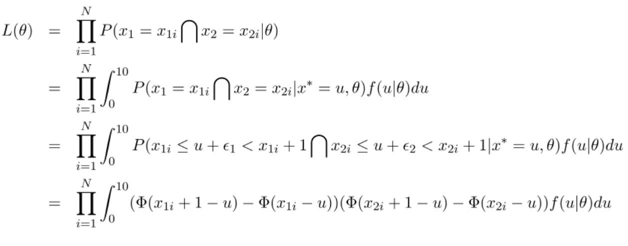
Likelihood function
Under our assumptions, we can determine for any θ the likelihood function that shows how likely it is that the parameter θ is the correct one given the assumed model and the observations. L(θ) = N ∏ i=1 P (x1= x1i ∩ x2 = x2i|θ) = N ∏ i=1 ∫ 10 0 P (x1 = x1i ∩ x2 = x2i|x∗= u, θ)f (u|θ)du = N ∏ i=1 ∫ 10 0 P (x1i≤ u + ϵ1< x1i+ 1 ∩ x2i≤ u + ϵ2< x2i+ 1|x∗ = u, θ)f (u|θ)du = N ∏ i=1 ∫ 10 0 (Φ(x1i+ 1− u) − Φ(x1i− u))(Φ(x2i+ 1− u) − Φ(x2i− u))f(u|θ)du Calibrations
We maximize the log-likelihood function to obtain the maximum-likelihood estimator:
θM ={mM, σMx , σϵM
} .
Table 2: Maximum-Likelihood Estimates
mM σM
x σMϵ
5.743 1.028 0.899 (0.093) (0.082) (0.052)
The data we collected in a replication study carried out at the ESSEC Experimental Lab in 2017 produce similar-sized estimates: see Appendix A.
4.
Simulations
Fictive outcomes and assumptions
Now that we have estimated the variance of the measurement error, as well as the mean and variance of the variable of interest x∗, we can use a simple linear stochastic model to simulate an outcome variable y∗ in order to evaluate the size of the measurement-error problem in simple OLS regressions, with particular emphasis on the value, significance and variance of the estimated coefficient. The simulations are carried out using the following
assumptions:
• y∗ = α + βx∗+ u x∗ ∼ N (mM, σxM2; [0, 10]) u∼ N (0, σu2) X∗⊥⊥ u
• x =⌊x∗+ ϵ⌋ with ϵ∼ N (0, σϵ2) X∗⊥⊥ ϵ ϵ⊥⊥ u
• σ2
u = 1
Under these assumptions and for the β we consider, we have Corr(y∗,x∗) ≃ β. Obviously Related Instrumental Variable
Gillen et al. (2019) argue convincingly that the test/retest design and the duplication of a noisy measure can help to correct attenuation bias and improve the significance of the estimated coefficients.
In a first step, they show that simple IV regressions (2SLS) using x1 as an instrument
for x2 (or the reverse) already improve the quality of the estimation.
To make the best use of all available information, and because there is no reason to prefer
x1 to instrument x2, or x2 to instrument x1, they combine the two IV regressions in one
convex combination, via a method they called Obviously Related Instrumental Variables. This requires that the errors in the 1st and 2nd measures be independent.
We will implement both the IV and the ORIV methods, which will allow us to emphasize the benefits of the latter. For ORIV, we estimate the stacked model:
y∗ y∗ = α1 α2 + β x1 x2 + u (1) instrumenting x1 x2 by W = x2 0N 0N x1
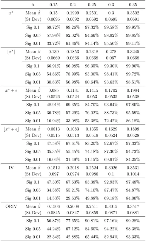
Table 3 displays the coefficient estimates from 100 000 simulated experiments with 100 subjects, a sample size that is relatively common in laboratory experiments. We use in the simulation five “actual” coefficients β = (0.15, 0.20, 0.25, 0.30, 0.35), of relatively small size, as these can be more sensitive to the measurement-error problem. The table shows the estimated mean, variances and frequencies of the significance of these estimators (at three error levels). We stack the estimates by the method of generating the latent variable (the true one, discretization, noise, and discretization and noise), and the estimation of the coefficient when the latent variable is noisy and truncated (IV and ORIV).
To help intuition, Figure 3 presents the distribution of the estimates for β = 0.25 in the six relevant simulations (the true variable, discretization, noise only, discretization and noise, simple IV and ORIV) for N=100; Table 4 displays the analogous estimates for a sample size of 200.
In Appendix B we provide coefficient estimates for “large” samples (up to N=1000), which appear much less frequently in laboratory experiments, but are common when using internet data collection through specialized platforms, or in some field studies.
Table 3: Simulations: Simple OLS and IV with N=100 (100 000 simulations) β 0.15 0.2 0.25 0.3 0.35 x∗ Mean ˆβ 0.1505 0.1998 0.2497 0.2999 0.3505 (St Dev) 0.0986 0.0985 0.099 0.099 0.0987 Sig 0.1 45.19% 64.69% 80.91% 91.40% 96.79% Sig 0.05 32.88% 52.41% 71.03% 85.26% 93.70% Sig 0.01 14.34% 28.42% 46.99% 66.17% 81.90% ⌊x∗⌋ Mean ˆβ 0.1395 0.185 0.2314 0.2779 0.3248 (St Dev) 0.095 0.0951 0.0955 0.0958 0.0954 Sig 0.1 42.94% 61.59% 78.10% 89.26% 95.65% Sig 0.05 30.94% 49.12% 67.64% 82.30% 91.77% Sig 0.01 13.18% 25.83% 43.12% 61.79% 77.89% x∗+ ϵ Mean ˆβ 0.0855 0.1131 0.1415 0.1699 0.1987 (St Dev) 0.0749 0.0748 0.0753 0.0761 0.0765 Sig 0.1 30.87% 44.71% 59.18% 72.18% 82.63% Sig 0.05 20.62% 32.53% 46.75% 60.70% 73.34% Sig 0.01 7.50% 14.02% 23.84% 36.12% 50.11% ⌊x∗+ ϵ⌋ Mean ˆβ 0.0818 0.1083 0.1355 0.1627 0.1902 (St Dev) 0.0732 0.0732 0.0737 0.0745 0.075 Sig 0.1 30.09% 43.24% 57.63% 70.61% 81.02% Sig 0.05 19.93% 31.28% 45.02% 58.84% 71.28% Sig 0.01 7.11% 13.35% 22.64% 34.32% 47.66% IV Mean ˆβ 0.1533 0.2028 0.2538 0.3057 0.3563 (St Dev) 0.1413 0.1427 0.1439 0.146 0.1478 Sig 0.1 28.69% 42.24% 56.78% 70.14% 81.03% Sig 0.05 18.10% 29.42% 43.16% 57.65% 70.61% Sig 0.01 5.14% 10.45% 19.08% 30.44% 43.78% ORIV Mean ˆβ 0.1521 0.2013 0.2518 0.3031 0.3536 (St Dev) 0.1218 0.1227 0.124 0.126 0.1273 Sig 0.1 36.52% 52.27% 67.80% 80.51% 89.32% Sig 0.05 25.27% 39.92% 55.66% 70.52% 82.12% Sig 0.01 10.17% 18.94% 31.75% 46.48% 61.58%
The first column indicates the variable or the estimation method used in the univariate OLS regression. The first variable is the true x∗, the second the discretization of the true variable, the third considers the effect of noise, the fourth combines noise and discretization. For the IV estimations, the discrete noisy measure⌊x∗
1+ ϵ⌋ is instrumented by ⌊x∗2+ ϵ⌋. For the ORIV estimations
the stack model uses⌊x∗j+ ϵ
⌋
for j∈ {1, 2}. The last five columns indicate the
average value, standard deviation and significance of β for 100 000 simulations. For instance the ORIV cell for Sig 0.1 and β = 0.15 is 36.52%, so that the estimated β using ORIV is significant in 36.52% of the 100 000 regressions at the 10% level when the true β is 0.15.
Table 4: Simulations: Simple OLS and IV with N=200 (100 000 simulations) β 0.15 0.2 0.25 0.3 0.35 x∗ Mean ˆβ 0.15 0.1999 0.2501 0.3 0.3502 (St Dev) 0.0695 0.0692 0.0692 0.0695 0.0691 Sig 0.1 69.72% 89.26% 97.32% 99.58% 99.95% Sig 0.05 57.98% 82.02% 94.66% 98.92% 99.85% Sig 0.01 33.72% 61.36% 84.14% 95.50% 99.11% ⌊x∗⌋ Mean ˆβ 0.139 0.1853 0.2318 0.278 0.3245 (St Dev) 0.0669 0.0666 0.0668 0.067 0.0668 Sig 0.1 66.91% 86.98% 96.35% 99.30% 99.90% Sig 0.05 54.86% 78.99% 93.00% 98.41% 99.72% Sig 0.01 30.83% 56.98% 80.64% 93.63% 98.51% x∗+ ϵ Mean ˆβ 0.085 0.1131 0.1415 0.1702 0.1984 (St Dev) 0.0526 0.0524 0.053 0.0535 0.0538 Sig 0.1 48.91% 69.35% 84.70% 93.64% 97.80% Sig 0.05 36.78% 57.29% 76.02% 88.73% 95.59% Sig 0.01 16.94% 33.08% 53.38% 72.42% 86.18% ⌊x∗+ ϵ⌋ Mean ˆβ 0.0813 0.1083 0.1355 0.1629 0.1899 (St Dev) 0.0515 0.0513 0.0519 0.0524 0.0528 Sig 0.1 47.58% 67.61% 83.20% 92.67% 97.33% Sig 0.05 35.35% 55.45% 74.18% 87.30% 94.73% Sig 0.01 16.04% 31.49% 51.15% 69.91% 84.25% IV Mean ˆβ 0.1512 0.2018 0.2524 0.3026 0.3531 (St Dev) 0.097 0.0974 0.0986 0.1 0.1014 Sig 0.1 47.30% 67.63% 83.38% 92.93% 97.48% Sig 0.05 34.58% 55.21% 74.10% 87.47% 94.87% Sig 0.01 14.53% 29.60% 49.88% 69.18% 84.00% ORIV Mean ˆβ 0.1506 0.2008 0.2511 0.3015 0.3517 (St Dev) 0.0845 0.0847 0.0859 0.0871 0.0881 Sig 0.1 56.87% 77.65% 90.81% 97.16% 99.28% Sig 0.05 44.24% 67.12% 84.60% 94.22% 98.38% Sig 0.01 22.34% 42.88% 65.44% 82.94% 93.33%
The first column indicates the variable or estimation method used in the uni-variate OLS regression. The first variable is the true x∗, the second the dis-cretization of the true variable, the third considers the effect of noise, the fourth combines noise and discretization. For the IV estimations, the discrete noisy measure⌊x∗
1+ ϵ⌋ is instrumented by ⌊x∗2+ ϵ⌋. For the ORIV estimations
the stack model uses⌊x∗j+ ϵ
⌋
for j ∈ {1, 2}. The last five columns indicate
the average value, standard deviation and significance of β for 100 000 sim-ulations. For instance the ORIV cell for Sig 0.1 and β = 0.15 is 56.87%, so that the estimated β using ORIV method is significant in 56.87% of the 100 000 regressions at the 10% level when the true β is 0.15.
Discussion of the results
(a) In line with theory, these simulations confirm that measurement error attenuates the coefficient of the variable of interest in univariate OLS regression: the “true” coefficient is approximately divided by 2. Increasing the size of the sample does not remove this bias, but does improve the significance of the coefficients.
(b) In small samples (N=100), measurement errors substantially affect the significance of the coefficients. For instance, with β = 0.25 the coefficient is significant at the 5% level only 46.75% of the time. This helps explain why the coefficients of “meaningful” variables by any theoretical standard are often insignificant in experimental research .
(c) The use of a discrete measure of a continuous variable of interest such as risk-aversion does not appear to be a major problem. As we can see from the simulation tables, this transformation only slightly reinforces the downward bias in the coefficients.
(d) For small samples (N=100) simple IV and ORIV estimations do not fully remove the measurement problem: while the bias is virtually eliminated, the frequency of insignificant coefficients is still very high (at 43 and 55 per cent, respectively, at the 5 per cent significance level).
(e) In larger samples (N=200) the ORIV estimator performs relatively well. Not only is the bias virtually eliminated, but significance is also improved (in particular as compared to the IV estimates). The ORIV coefficients are slightly upward-biased due to the discrete transformation of the observations. See Appendix B for an comparative performance analysis of IV and ORIV in large samples (N=1000).
The frequency curves in Figure 3 depict the distribution of the estimated coefficients (for beta=0.25, and N=100). These show that: (1) the main source of the bias is the measurement error; (2) the discrete transformation of the continuous variable of interest does not much shift the distribution; and (3) the ORIV method eliminates the bias but produces a higher variance.
0 2 4 0.0 0.5 density X. X. X.+ ε X.+ ε IV ORIV
Figure 3: The distribution of the estimators for β = 0.25 and N=100
5.
Conclusion
By cutting the estimated coefficients in half and substantially reducing their significance, the problem of measurement error appears too large to be ignored. For instance, the pro-portion of regressions in which the coefficient of risk aversion appear significant is roughly divided by two for N=200 for a significance level of 0.01. As a consequence, the external validity of measures of risk-aversion is greatly undermined. While we here focus on the Holt-Laury method - the most popular method - there is no reason to believe that different elicitation methods would not lead to similar results.
Our results of course depend on simplifying assumptions that are made throughout the text. While many of these are quite standard (such as assuming that the variable of interest and the error terms are normally-distributed) others can be criticized. In particular, we assumed that the errors in the two repeated tasks are orthogonal. We furthermore ruled out the possibility of an individual switching back and forth in HL-like tasks, even though this behavior is often observed in practice. However, we do not feel that alternative assumptions would have dramatically changed our conclusions: intra-subject variability is too large to be ignored as a cause of measurement error.
within-subject measures in test/retest data, which is now well-documented. In particular, the task used to elicit risk-aversion, as well as the delay between the test and the retest, have little influence on the importance of intra-subject variability, which remains large in all instances.8
A second lesson from our work here relates to sample size. The problems arise when the sample is of the size typical in experimental economics. Most of the significance issues disappear with N = 1000. Since it may be too costly to systematically increase sample sizes up to this value, we suggest the use of IV or ORIV estimation, which corrects most problems for N over 200. Smaller samples are definitely prone to measurement errors, and the results regarding the significance of the risk-aversion coefficient should be interpreted cautiously. This requires eliciting two measures of the variable of interest (risk-aversion in our case), which is probably less costly than doubling or tripling the sample size.
Within the framework of these simplifying assumptions, our study should be seen as a first attempt to use test/retest data to determine the size of the measurement error in probably the most popular risk-aversion elicitation task to date. It also provides new evidence supporting the use of the ORIV method.
References
Attanasi, G., N. Georgantzís, V. Rotondi, and D. Vigani (2018). Lottery-and survey-based risk attitudes linked through a multichoice elicitation task. Theory and Decision 84(3), 341–372.
Bardsley, N., R. Cubitt, G. Loomes, P. Moffat, C. Starmer, and R. Sugden (2010).
Experi-mental Economics: Rethinking the Rules. Princeton University Press.
Charness, G., T. Garcia, T. Offerman, and M. Villeval (2019). Do measures of risk attitude in the laboratory predict behavior under risk in and outside of the laboratory? GATE
Working Paper No. 1921.
Chuang, Y. and L. Schechter (2015). Stability of experimental and survey measures of risk, time, and social preferences: A review and some new results. Journal of Development
Economics 117, 151–170.
Crosetto, P. and A. Filippin (2016). A theoretical and experimental appraisal of four risk elicitation methods. Experimental Economics 19(3), 613–641.
8See Chuang and Schechter (2015), Reynaud and Couture (2012), Crosetto and Filippin (2016),
Engel, C. and O. Kirchakamp (2019). How to deal with inconsistent choices on multiple price lists. Journal of Economic Behavior and Organization 160, 138–157.
Frederick, S. (2005, December). Cognitive reflection and decision making. Journal of
Eco-nomic Perspectives 19(4), 25–42.
Gillen, B., E. Snowberg, and L. Yariv (2019). Experimenting with measurement error: Tech-niques with applications to the Caltech cohort study. Journal of Political Economy 127 (4), 1826–1863.
Hey, J. D., A. Morone, and U. Schmidt (2009). Noise and bias in eliciting preferences.
Journal of Risk and Uncertainty 39(3), 213–235.
Holt, C. A. and S. K. Laury (2002). Risk aversion and incentive effects. American Economic
Review 92(5), 1644–1655.
Jacobson, S. and R. Petrie (2009). Learning from mistakes: What do inconsistent choices over risk tell us? Journal of Risk and Uncertainty 38(2), 143–158.
Mata, R., R. Frey, D. Richter, J. Schupp, and R. Hertwig (2018). Risk preference: A view from psychology. Journal of Economic Perspectives 32(2), 155–72.
O’Donoghue, T. and J. Somerville (2018, May). Modeling risk aversion in economics. Journal
of Economic Perspectives 32(2), 91–114.
Reynaud, A. and S. Couture (2012). Stability of risk preference measures: results from a field experiment on french farmers. Theory and Decision 73(2), 203–221.
Schildberg-Hörisch, H. (2018). Are risk preferences stable? Journal of Economic
Perspec-tives 32(2), 135–54.
Zhou, W. and J. Hey (2018). Context matters. Experimental Economics 21(4), 723–756.
Appendix A. A replication of HL
We replicated the HL test/retest procedure in 2019, with a total of 60 participants in three experimental sessions organized at the ESSEC Experimental Lab (France). Subjects made their decisions on a computer screen and could not establish eye contact with one another; the instructions and data collection were computerized.
The experiment included a first HL risk-elicitation task (Table 1), two attention-diversion tasks (lasting for approximately 10 minutes) and a second HL risk-elicitation task, identical to the first.
The first diversion was the CRT (cognitive-reflection task) introduced by Frederick (2005). The second was a simple real-effort task (counting 7’s) that subjects had to carry out for four minutes. These tasks were not incentivized.
Subjects also indicated their age, gender and major track in their Secondary education. The payoffs for the session are based on the results from one randomly-selected risk task. The session lasted approximately 20 minutes and participants earned on average 7 Euros.
Note that the frequency of multiple switches in these data is very low, at under 5 percent.
0 .05 .1 .15 .2 .25 Density 0 2 4 6 8 10 1st repetition 0 .05 .1 .15 .2 .25 Density 2 4 6 8 10 2nd repetition
Figure 4: The number of safe choices in the two repetitions of the HL task in the ESSEC replication study
Table 5: Maximum-Likelihood Estimates for the ESSEC students
mM σMx σMϵ
6.205 1.319 1.092 (0.199) (0.182) (0.103)
Appendix B. Simulations for “large” samples
In this Appendix we provide estimates for “large” samples: N=300, N=500 and N=1000 (over 10000 simulations).
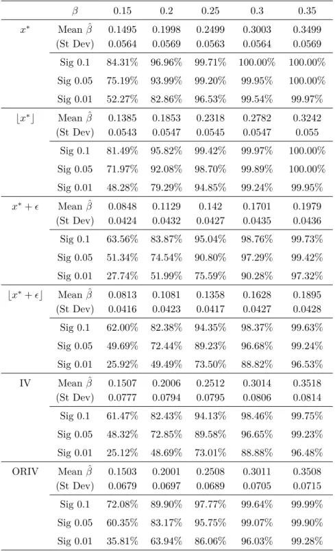
Table 6: Simulations: Simple OLS and IV with N=300 (10 000 simulations) β 0.15 0.2 0.25 0.3 0.35 x∗ Mean ˆβ 0.1495 0.1998 0.2499 0.3003 0.3499 (St Dev) 0.0564 0.0569 0.0563 0.0564 0.0569 Sig 0.1 84.31% 96.96% 99.71% 100.00% 100.00% Sig 0.05 75.19% 93.99% 99.20% 99.95% 100.00% Sig 0.01 52.27% 82.86% 96.53% 99.54% 99.97% ⌊x∗⌋ Mean ˆβ 0.1385 0.1853 0.2318 0.2782 0.3242 (St Dev) 0.0543 0.0547 0.0545 0.0547 0.055 Sig 0.1 81.49% 95.82% 99.42% 99.97% 100.00% Sig 0.05 71.97% 92.08% 98.70% 99.89% 100.00% Sig 0.01 48.28% 79.29% 94.85% 99.24% 99.95% x∗+ ϵ Mean ˆβ 0.0848 0.1129 0.142 0.1701 0.1979 (St Dev) 0.0424 0.0432 0.0427 0.0435 0.0436 Sig 0.1 63.56% 83.87% 95.04% 98.76% 99.73% Sig 0.05 51.34% 74.54% 90.80% 97.29% 99.42% Sig 0.01 27.74% 51.99% 75.59% 90.28% 97.32% ⌊x∗+ ϵ⌋ Mean ˆβ 0.0813 0.1081 0.1358 0.1628 0.1895 (St Dev) 0.0416 0.0423 0.0417 0.0427 0.0428 Sig 0.1 62.00% 82.38% 94.35% 98.37% 99.63% Sig 0.05 49.69% 72.44% 89.23% 96.68% 99.24% Sig 0.01 25.92% 49.49% 73.50% 88.82% 96.53% IV Mean ˆβ 0.1507 0.2006 0.2512 0.3014 0.3518 (St Dev) 0.0777 0.0794 0.0795 0.0806 0.0814 Sig 0.1 61.47% 82.43% 94.13% 98.46% 99.75% Sig 0.05 48.32% 72.85% 89.58% 96.65% 99.23% Sig 0.01 25.12% 48.69% 73.01% 88.88% 96.48% ORIV Mean ˆβ 0.1503 0.2001 0.2508 0.3011 0.3508 (St Dev) 0.0679 0.0697 0.0689 0.0705 0.0715 Sig 0.1 72.08% 89.90% 97.77% 99.64% 99.99% Sig 0.05 60.35% 83.17% 95.75% 99.07% 99.90% Sig 0.01 35.81% 63.94% 86.06% 96.03% 99.28%
The first column indicates the variable or estimation method used in the uni-variate OLS regression. The first variable is the true x∗, the second the dis-cretization of the true variable, the third considers the effect of noise, the fourth combines noise and discretization. For the IV estimations, the discrete noisy measure⌊x∗
1+ ϵ⌋ is instrumented by ⌊x∗2+ ϵ⌋. For the ORIV estimations
the stack model uses⌊x∗j+ ϵ
⌋
for j ∈ {1, 2}. The last five columns indicate
the average value, standard deviation and significance of β for 10 000 simu-lations. For instance the ORIV cell for Sig 0.1 and β = 0.15 is 72.08%, so that the estimated β using ORIV method is significant in 72.08% of the 10 000 regressions at the 10% level when the true β is 0.15.
Table 7: Simulation: Simple OLS and IV with N=500 (10 000 simulations) β 0.15 0.2 0.25 0.3 0.35 x∗ Mean ˆβ 0.1506 0.1999 0.2504 0.3003 0.3498 (St Dev) 0.0435 0.0438 0.0438 0.0438 0.0441 Sig 0.1 96.46% 99.76% 99.99% 100.00% 100.00% Sig 0.05 93.06% 99.51% 99.97% 100.00% 100.00% Sig 0.01 80.32% 97.60% 99.90% 100.00% 100.00% ⌊x∗⌋ Mean ˆβ 0.1394 0.1854 0.2321 0.2784 0.3242 (St Dev) 0.0421 0.0423 0.0425 0.0423 0.0425 Sig 0.1 95.16% 99.62% 99.98% 100.00% 100.00% Sig 0.05 90.96% 99.22% 99.95% 100.00% 100.00% Sig 0.01 76.32% 96.39% 99.79% 100.00% 100.00% x∗+ ϵ Mean ˆβ 0.0852 0.1134 0.1419 0.1704 0.198 (St Dev) 0.033 0.0331 0.0332 0.0337 0.0338 Sig 0.1 82.56% 96.21% 99.46% 99.98% 100.00% Sig 0.05 72.80% 92.63% 98.74% 99.89% 100.00% Sig 0.01 50.01% 79.99% 95.10% 99.29% 99.94% ⌊x∗+ ϵ⌋ Mean ˆβ 0.0814 0.1086 0.1358 0.1631 0.1894 (St Dev) 0.0323 0.0324 0.0325 0.033 0.0331 Sig 0.1 80.73% 95.43% 99.34% 99.98% 100.00% Sig 0.05 71.03% 91.49% 98.52% 99.87% 99.99% Sig 0.01 47.48% 77.86% 94.08% 99.06% 99.89% IV Mean ˆβ 0.1513 0.2003 0.2508 0.3017 0.3505 (St Dev) 0.0607 0.0608 0.0614 0.0622 0.0639 Sig 0.1 80.87% 95.76% 99.40% 99.92% 100.00% Sig 0.05 71.45% 91.74% 98.73% 99.82% 100.00% Sig 0.01 47.63% 77.17% 94.30% 99.13% 99.94% ORIV Mean ˆβ 0.1506 0.2003 0.2506 0.3013 0.3499 (St Dev) 0.0528 0.0534 0.0536 0.0543 0.0556 Sig 0.1 89.45% 98.29% 99.86% 100.00% 100.00% Sig 0.05 82.11% 96.84% 99.70% 99.99% 100.00% Sig 0.01 61.75% 89.13% 98.42% 99.89% 100.00%
The first column indicates the variable or estimation method used in the uni-variate OLS regression. The first variable is the true x∗, the second the dis-cretization of the true variable, the third considers the effect of noise, the fourth combines noise and discretization. For the IV estimations, the discrete noisy measure⌊x∗
1+ ϵ⌋ is instrumented by ⌊x∗2+ ϵ⌋. For the ORIV estimations
the stack model uses⌊x∗j+ ϵ
⌋
for j ∈ {1, 2}. The last five columns indicate
the average value, standard deviation and significance of β for 10 000 simu-lations. For instance the ORIV cell for Sig 0.1 and β = 0.15 is 89.45%, so that the estimated β using ORIV method is significant in 89.45% of the 10 000 regressions at the 10% level when the true β is 0.15.
Table 8: Simulation: Simple OLS and IV with N=1000 (10 000 simulations) β 0.15 0.2 0.25 0.3 0.35 x∗ Mean ˆβ 0.1501 0.2001 0.2497 0.3004 0.3497 (St Dev) 0.0305 0.0313 0.0308 0.0305 0.0308 Sig 0.1 99.97% 100.00% 100.00% 100.00% 100.00% Sig 0.05 99.88% 99.99% 100.00% 100.00% 100.00% Sig 0.01 99.11% 99.99% 100.00% 100.00% 100.00% ⌊x∗⌋ Mean ˆβ 0.1392 0.1854 0.2316 0.2784 0.3242 (St Dev) 0.0293 0.0301 0.0295 0.0294 0.0296 Sig 0.1 99.92% 99.99% 100.00% 100.00% 100.00% Sig 0.05 99.76% 99.98% 100.00% 100.00% 100.00% Sig 0.01 98.59% 99.96% 100.00% 100.00% 100.00% x∗+ ϵ Mean ˆβ 0.0852 0.1136 0.1416 0.1702 0.1982 (St Dev) 0.0231 0.0236 0.0236 0.0233 0.0239 Sig 0.1 97.97% 99.91% 100.00% 100.00% 100.00% Sig 0.05 95.67% 99.82% 100.00% 100.00% 100.00% Sig 0.01 85.42% 98.61% 99.94% 100.00% 100.00% ⌊x∗+ ϵ⌋ Mean ˆβ 0.0815 0.1086 0.1355 0.163 0.1896 (St Dev) 0.0227 0.023 0.023 0.0229 0.0234 Sig 0.1 97.56% 99.89% 100.00% 100.00% 100.00% Sig 0.05 95.04% 99.65% 100.00% 100.00% 100.00% Sig 0.01 83.69% 98.32% 99.91% 100.00% 100.00% IV Mean ˆβ 0.1505 0.2006 0.2502 0.3009 0.3499 (St Dev) 0.0422 0.0435 0.0433 0.0436 0.0441 Sig 0.1 97.20% 99.85% 100.00% 100.00% 100.00% Sig 0.05 94.53% 99.61% 100.00% 100.00% 100.00% Sig 0.01 83.84% 98.26% 99.97% 100.00% 100.00% ORIV Mean ˆβ 0.1504 0.2005 0.2501 0.3006 0.3498 (St Dev) 0.037 0.0379 0.0378 0.0379 0.0388 Sig 0.1 99.27% 99.96% 100.00% 100.00% 100.00% Sig 0.05 98.34% 99.93% 100.00% 100.00% 100.00% Sig 0.01 93.27% 99.67% 99.99% 100.00% 100.00%
The first column indicates the variable or estimation method used in the uni-variate OLS regression. The first variable is the true x∗, the second the dis-cretization of the true variable, the third considers the effect of noise, the fourth combines noise and discretization. For the IV estimations, the discrete noisy measure⌊x∗
1+ ϵ⌋ is instrumented by ⌊x∗2+ ϵ⌋. For the ORIV estimations
the stack model uses⌊x∗j+ ϵ
⌋
for j∈ {1, 2}. The last five columns indicate the
average value, standard deviation and significance of β for 10 000 simulations. For instance the IV cell for Sig 0.1 and β = 0.15 is 97.20%s, so that the esti-mated β using ORIV method is significant in 97.20% of the 10 000 regressions at the 10% level when the true β is 0.15.
C O N T A C T
RESEARCH CENTER