HAL Id: tel-01439268
https://tel.archives-ouvertes.fr/tel-01439268
Submitted on 18 Jan 2017HAL is a multi-disciplinary open access
archive for the deposit and dissemination of sci-entific research documents, whether they are pub-lished or not. The documents may come from teaching and research institutions in France or abroad, or from public or private research centers.
L’archive ouverte pluridisciplinaire HAL, est destinée au dépôt et à la diffusion de documents scientifiques de niveau recherche, publiés ou non, émanant des établissements d’enseignement et de recherche français ou étrangers, des laboratoires publics ou privés.
Évolution de l’évolution de l’occupation du sol
(1950-2025) et impacts sur l’érosion du sol dans un
bassin versant méditerranéen
Hari Gobinda Roy
To cite this version:
Hari Gobinda Roy. Évolution de l’évolution de l’occupation du sol (1950-2025) et impacts sur l’érosion du sol dans un bassin versant méditerranéen. Géographie. Université Côte d’Azur, 2016. Français. �NNT : 2016AZUR2024�. �tel-01439268�
THESE
présentée devant
l’Université de Nice - Sophia Antipolis
en vue de l’obtention du
DIPLÔME DE DOCTORAT
(arrêté ministériel du 30 mars 1992)Spécialité : Géographie
par
Hari Gobinda ROY
Long term prediction of soil erosion (1950-2025) in a Mediterranean context of
rapid urban growth and land cover change
Evolution de l’évolution de l’occupation du sol (1950-2025) et impacts sur
l’érosion du sol dans un bassin versant méditerranéen
Soutenue le 15 septembre 2016 Membres du Jury :
Pr Pierre CARREGA
Examinateur
Pr Dennis FOX
Directeur
Pr Catherine MERING
Rapporteur
Pr Laurent RIEUTORT
Rapporteur
Pr Yves BAUDOUIN
Examinateur
UMR ESPACE 7300 CNRS
Equipe Gestion et Valorisation de l’Environnement
i
ABSTRACT
The European Mediterranean coastal area has experienced widespread land cover change since 1950 because of rapid urban growth and expansion of tourism. Urban sprawl and other land cover changes occurred due to post-war economic conditions, population migration, and increased tourism. Land cover change has occurred through the interaction of environmental and socio-economic factors, including population growth, urban sprawl, industrial development, and environmental policies. In addition, rapid expansion of tourism during the last six decades has caused significant socioeconomic changes driving land cover change in Euro-Mediterranean areas. Mediterranean countries from Spain to Greece experienced strong urban growth from the
1970’s onwards, and a moderate growth rate is projected to continue into the future. Land cover
change can result in environmental changes such as water pollution and soil degradation. Several previous studies have shown that Mediterranean vineyards are particularly vulnerable to soil erosion because of high rainfall intensity and the fact that vineyards are commonly located on steeper slopes and the soil is kept bare during most of the cultivation period (November to April) when precipitation is at its highest.
To date, few Euro-Mediterranean studies of land cover change explicitly explore spatial constraints on land cover change patterns. Many modeling tools have been developed to explore and evaluate future land cover change possibilities, and time scales have varied greatly from one study to another. Most LUCC models relate change to physical and socio-economic factors in a grid of cells.
The main objective of this thesis is to predict long-term soil erosion evolution in a Mediterranean context of rapid urban growth and land use change at the catchment scale. In order to achieve this, the following specific aims have been formulated: (i) to analyze the spatial dynamics of land cover change from 1950 to 2008; (ii) to compare the impact of historical time periods on land cover prediction using different time scales; (iii) to test the impacts of spatial extent and cell size on LUCC modeling; and (iv) to predict the impact of land cover change on soil erosion for 2025.
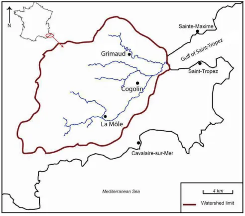
The study area of approximately 235 km² is situated in the Var, a department located in southeastern France near the Gulf of St. Tropez. The western and higher part of the watershed,
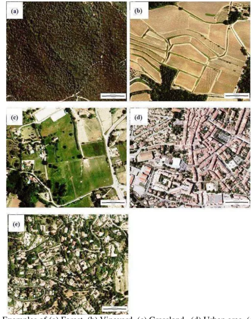
ii consisting of about 70% of the catchment, is mostly pine and oak forest; the topography is uneven with the highest elevation at about 650 m. The eastern and lower part of the catchment is a gently sloping alluvial plain. The catchment area is characterized by a Mediterranean climate with hot, dry summers and cooler, rainy winters. Land cover maps were screen-digitized from digital orthorectified aerial photographs (1950, 1982, 2003, 2008, & 2011) purchased from the Institut Géographique National. In order to determine past land cover change patterns, surfaces were classified into five land cover categories based on visual interpretation, namely forest, vineyard, grassland, urban, and suburban. To analyze the spatial dynamics of past land cover change and create a model to predict future land cover change, surfaces were simplified into four categories, namely forest, vineyard, grassland, and built area. (Urban and suburban areas were combined into built area due to their small amount of coverage compared to other land cover categories.) Finally, soil erosion was predicted for the vineyard category.
The aerial photographs from 1950 were the first high-quality post-Second World War photographs available when the area was still largely rural. An intermediate date of 1982 was selected between 1950 and the most recent photographs. Aerial photographs from 1982 represent land cover conditions at the beginning of rapid urban sprawl. Cell size of all digitized maps was changed from 1 m to 25 m to make land cover layers compatible with the 25 m DEM used for the creation of topographic and distance variables.
Land cover change was analyzed using the Land Change Modeler (LCM) and CROSSTAB
modules of IDRISI (Eastman, 2012). Explanatory variables were selected through Cramer’s
coefficient. Land cover maps for 2011 were predicted using three different time scales, namely 1950-1982, 1982-2003, and 2003-2008. These predictions were then compared to the actual digitized land cover map from 2011 to evaluate model accuracy. Major topographic and distance variables were identified including the following: slope, altitude, distance from roads, distance from built area in initial year, and distance from streams. In addition, three constraints and incentives-- forest to built area, vineyard to built area, and grassland to built area-- were included in the prediction process. These were created from the Plan Local d’Urbanisme (PLU) and the
Schéma de Cohérence Territoriale (SCOT). Kappa index and confusion matrix were used to evaluate the model’s accuracy. LCM of IDRISI was used to predict land cover in 2011.
iii LCC dynamics, both in terms of absolute and relative change, were first analyzed using intensity analysis. Then land cover was predicted for 2011 for large (79.1 km²) and small (36.6 km²) windows using cell sizes of 25 m, 50 m, 100 m. Spatial resolution effects were also analyzed by upscaling from 25 m to 50 m and 100 m and then downscaling back to 25 m. Here spatial extent is equivalent to increasing the proportional area of a dormant category. Two spatial extents (36.6 km² and 79.1 km²) and three resolutions (25 m, 50 m and 100 m) were tested. The 50 m and 100 m resolutions were downscaled back to 25 m. Land cover maps dated from 1950, 1982, 2003 and 2011, and LCM was used to predict 2011 cover. Finally, RUSLE was used to predict soil erosion for different years: 1950, 1982, 2003, 2011, and 2025 (predicted).
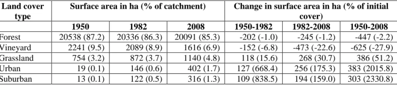
This study found that land cover changes were concentrated mainly in the alluvial plain and adjoining foothills. Forest remained the dominant land cover in the catchment, changing only slightly from around 86% to 85% in 1950-2008. However, forested areas underwent significant swapping with vineyard and grassland areas. The catchment experienced a marked decrease in vineyard (-28%) and a substantial increase in grassland (about +50%). Urban and suburban areas remained a minor component of the catchment (about 3%), but showed a dramatic relative increase (more than 20 times initial cover). Built areas grew at the expense of vineyards, and grassland also increased on former vineyards. Losses in vineyard were offset in part by growth of vineyard on previously forested foothills close to the alluvial plain. This finding differs from other Mediterranean studies that have shown agriculture (i.e. vineyard cultivation), in the face of urban pressure, moving to steeper marginal slopes, while abandoning fertile plain soils to grassland and forest. Topography (altitude, slope) and distance variables (from roads, streams, built area, and the sea) strongly influenced land cover change dynamics in the catchment between 1950 and 2008. Vineyard located near streams was converted mainly to grassland. Built areas were strongly dependent on roads and former built areas for expansion but expanded little near streams due to flooding risks. Finally, the rate of change was greater during the latter part of the study (1982-2008) than in the earlier period (1950-1982).
Kappa index and confusion matrix were used to evaluate the model’s accuracy. Altitude, slope, and distance from roads had the greatest impact on land cover changes among all variables tested. Good to perfect level of spatial agreement and perfect level of quantitative agreement were observed in long to short time scale simulations. Kappa indices (Kquantity = 0.99 and Klocation
iv = 0.90) and confusion matrices were good for intermediate and best for short time scale. The results indicate that shorter time scales produce better predictions. Time scale effects have strong interactions with specific land cover dynamics; for example, stable land cover categories are easier to predict than rapidly changing ones, and overall quantity is easier to predict than specific location over longer time periods.
Spatial extent had a major impact on land cover change dynamics as absolute and relative values of gains/losses were inverted when dormant category increased. It also improved Cramer’s V values (1.3 to 1.5 times greater) and disagreement values artificially improved (twice as good) in change prediction; this resulted from an increase in the number of correctly classified persistent cells. Upscaling/downscaling revealed that coarser cell sizes lose considerable predictive power (1.5 to 2 times greater allocation errors), despite validation statistics. In future studies, dormant category area should be minimized and upscaling/downscaling should be done if data are modeled at coarser resolutions than original cell size.
Land use changes were found to have a significant impact on soil erosion rates in different years. Between 1950 and 2003, soil erosion prone areas increased in the eastern and central parts of the study area; there was decreased soil erosion in the north and western parts of the catchment due a shift from vineyard to built area in the alluvial plain area. Vineyard decreased in the alluvial plain land, and increased in the upland valley and foothills. Therefore, mean and median slope values increased moderately in the same time period. A positive relationship between slope gradient and erosion rates in different years (1950, 1982 & 2003) was observed in this study.
v
Table of Contents
Abstract ... i
GENERAL INTRODUCTION ... 1
PURPOSE OF THE STUDY ... 1
STATEMENT OF PROBLEM ... 3
ORGANIZATION OF THE THESIS ... 3
CHAPTER 1 7 LITERATURE REVIEW ON LAND COVER CHANGE DYNAMICS AND LAND COVER CHANGE MODELING 1 Land cover change ... 7
1.1 Major trends of land cover change ... 8
1.2 Factor affecting land cover change ... 12
1.2.1 Demographic pressure and urban sprawl ... 12
1.2.2 Tourism ... 14
1.2.3 Intensification of agriculture ... 16
1.2.4 Land abandonment ... Erreur ! Signet non défini. 1.2.5 Economic factors ... 20
1.2.6 Policy and planning ... 21
1.1.3.6 Results of land abandonment ... 21
1.3 Land cover chnage conclusion ... 22
PART 2: LITERATURE REVIEW ON LAND COVER CHANGE MODELING Erreur ! Signet non défini. 2 Land cover change modeling ... 23
2.1 Land cover and land use change models ... 24
2.2 Cellular Automata (CA) ... 25
2.2.1 Fundamental components of a CA model ... 26
2.2.2 CA models in Geography ... 27
2.2.3 SLEUTH model ... 28
vi
2.2.5 Urban Expansion Dynamic (UED) model ... 31
2.2.6 Advantages and limitations of CA models Erreur ! Signet non défini. 2.3 Markov chain modeling ... 32
2.4 Markov-CA model ... 34
2.5 IDRISI-Land Change Modeler (LCM) model ... 36
2.5.1 Literature review on IDRISI-LCM ... 38
2.6 Agent based modeling (ABM) in Geography ... 41
2.7 Model choice ... 43
2.8 Conclusion ... 45
CHAPTER 2 46 1 Introduction ... 46
2 Methods ... 48
2.1 The study area ... 48
2.2 Data description and land cover classification ... 50
2.3 Cross tabulation analysis in 1950-1982, 1982-2008, and 1950-2008 Erreur ! Signet non défini. 2.4 Spatial dynamics ... 52
3 Results ... 53
3.1 Areal trends in land cover change ... 53
3.1.1 Cross tabulation analysis 1950-1982 ... 55
3.1.2 Cross tabulation analysis 1982-2008 ... 56
3.1.3 Cross tabulation analysis 1950-2008 ... 58
3.2 Spatial dynamics influencing land cover change ... 59
3.2.1 General spatial trends ... 59
3.2.2 Altitude ... 61
3.2.3 Slope ... 64
3.2.4 Distance from streams ... 66
3.2.5 Distance from roads ... 68
3.2.6 Distance from built area ... 70
vii
4 Discussion ... 74
2.5 Conclusion ... 78
CHAPTER 3 34 1 Introduction ... 79
1.1 Land cover change modeling ... 79
1.2 The role of time scale in land change prediction ... 81
1.3 Objectives ... 82
2 Methods ... 82
2.1 Site description ... 82
2.2 Land change modeling procedure ... 83
2.2.1 Digital data and land cover categories ... 84
2.2.2 Explanatory variables and constraints ... 85
2.2.3 Selection of explanatory variables ... 87
2.2.4 Transition potentials ... 87
2.2.5 Land cover prediction and time scales test ... 88
2.2.6 Land cover prediction validation ... 88
3 RESULTS ... 91
3.1 Land cover change analysis during different time periods ... 91
3.2 Selection of explanatory variables ... 94
3.3 Transition potentials ... 96
3.4 Prediction of land cover change using different time scales ... 100
3.5 Validation of predicted land cover ... 102
3.5.1 Kappa index analysis for predicted land cover from different time periods ... 103
3.5.2 Error matrix analysis for predicted land cover from different time periods ... 104
viii 4 Discussion ... 105 5 Conclusion ... 107 CHAPTER 4 108 1 Introduction ... 108 2 Methods ... 116 2.1 Site description ... 116
2.2 Intensity of land cover change ... 117
2.2.1 Interval intensity analysis ... 118
2.2.2 Category intensity analysis ... 118
2.2.3 Transition intensity analysis ... 118
2.3 Land cover change modelling steps ... 119
2.3.1 Land cover mapping ... 119
2.3.2 Independent variables and constraints ... 120
2.3.3 Explanatory variables and creating transition potential statistics 121 2.3.4 Land cover simulation ... 122
2.3.5 Validation of predicted land cover maps ... 122
3 Results ... 122
3.1 Land cover maps and category areas in the small and large zones 122
3.2 Land cover change intensity ... 125
3.2.1 Interval intensity analysis ... 125
3.2.2 Category intensity analysis ... 126
3.2.3 Transition intensity analysis ... 129
3.3 Dormant category impacts on land modeling indices ... 133
3.3.1 Cramer’s V ... 134
3.3.2 Prediction validation ... 135
3.4 Cell size impacts on land cover modelling indices ... 136
4 Discussion ... 138
4.1 Perception of land cover change dynamics and spatial extent 138
ix
4.3 Spatial resolution and change prediction ... 141
5 Conclusion ... 142
CHAPTER 5 98 1 Introduction ... 143
1.1 Factors affecting soil erosion ... 144
1.2 The magnitude of erosion in the Mediterranean Europe ... 146
1.3 Soil erosion in the Mediterranean vineyard ... 147
1.4 Soil erosion models ... 148
1.4.1The use of RUSLE model in different studies ... 149
1.4.2RUSLE model description ... 151
1.4.2.1 Rainfall-Runoff erosivity factor (R) ... 151
1.4.2.2 Soil erodibility factor (K) ... 152
1.4.2.3 Topographic factor (Slope length and slope steepness) (LS) 152 1.4.2.4 Cover management factor ... 154
1.4.2.5 Conservation practice (P) factor ... 155
1.5 Objectives ... 155
2 Methods ... 156
2.1 Site description ... 156
2.2 Erosion estimation using RUSLE ... 156
2.2.1 RUSLE parameters for soil erosion estimation ... 157
2.2.1.1 Rainfall-Runoff erosivity factor (R) ... 157
2.2.1.2 Soil erodibility factor (K) ... 157
2.2.1.3 Topographic factor (Slope length and slope steepness) (LS) 157 2.2.1.4 Cover management factor (C) ... 158
2.2.1.5Conservation practice P factor ... 158
2.2.2 Soil erosion mapping and validation ... 158
2.3 Land cover prediction for 2025 ... 158
3 Results and Discussion ... 159
3.1 Changes in vineyard area ... 159
x
3.3 Soil erosion in the catchment ... 163
5.5 Conclusion ... 168
GENERAL CONCLUSION ... 123
Synthesis ... 168
Limitations of the study ... 170
Suggestions for future research ... 170
REFERENCES ... 171
APPENDIX 1: Résumé long en français ... 184
xi
List of Tables
Table 2.1: Surface area of land cover types for 1950, 1982, and 2008, and changes in area for
1950-1982, 1982-2008, and 1950-2008. ... 8
Table 2.2: Cross-tabulation of land cover in 1950 (columns) and in 1982 (rows). Values are in ha, persistence (diagonal) is also expressed in % of total area in initial year (1950). ... 10
Table 2.3: Summary of land cover changes (1950-1982) expressed as % of catchment. ... 11
Table 2.4: Cross-tabulation of land cover in 1982 (columns) and in 2008 (rows). Values are in ha, persistence (diagonal) is also expressed in % of total area in initial year (1982). ... 12
Table 2.5: Summary of land cover changes (1982-2008) expressed as % of catchment. ... 12
Table 2.6: Cross-tabulation of land cover 1950 (columns) and land cover 2008 (rows) (ha) ... 13
Table 2.7: Summary of land cover changes (1950-2008) expressed as % of catchment. ... 14
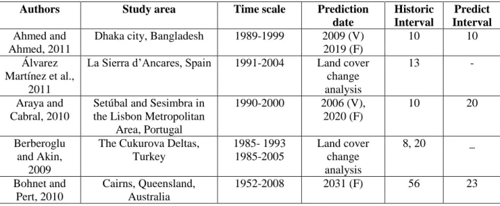
Table 3.1: Temporal scales of different studies. (V- Year of validation, F- year of future prediction) ... 35
Table 3.2: Characteristics of the different land cover classes ... 40
Table 3.3: Historical time periods, prediction and validation dates for different scales. ... 43
Table 3.4: Level of agreement associated with Kappa values by (Landis and Koch 1977) ... 44
Table 3.5: Percentage of the catchment area for each category ... 48
Table 3.6: Cramer’s V coefficient (relationship between land cover change and explanatory variables). Values ≥ 0.40 are highlighted in bold. ... 51
Table 3.7: Accuracy rate (%) of transition potentials in different time periods (F-Forest, V-Vineyard, G-Grassland, B-Built area). ... 55
Table 3.8. Land cover transition probabilities in 1982-201, 2003-2011, and 2008-2011, using different time periods 1950-1982, 1982-2003, and 2003-2008, respectively. Expected transition area or change area matrix is also expressed in ha in diagonal, accounted from the total area in initial year (T2). ... 57
Table 3.9: Summary of Kappa indices ... 59
Table 3.10: Error matrix analysis of actual land cover map 2011 (Column) against predicted land cover from transition potentials for different time periods. Values are expressed in hectares (ha) and error of commission and omission are expressed in % and in bold. ... 60
Table 4.1: Spatial scales, land cover types, and variables of different studies ... 65
Table 4.2: Surface area of land cover types for different years. Values are expressed in ha (% of catchment area is noted in parentheses). ... 78
Table 4.3: Category land cover and total change during the different time intervals, and % of change occurring in the small window (equal to 100% everywhere for the top rows). ... 80
xii
Table 4.4: Cramer’s V coefficient for 25 m cell size. Values ≥ 0.40 are highlighted in bold and
overall accuracy is in italics ... 89
Table 4.5: Cramer’s V coefficient for 50 m cell size. Values ≥ 0.40 are highlighted in bold and
overall accuracy is in italics ... 90
Table 4.6: Cramer’s V coefficient for 100 m cell size. Values ≥ 0.40 are highlighted in bold and
overall accuracy is in italics ... 90
Table 4.7: Cramer’s V coefficient for 50-25 m upscaling/downscaling cell size. Values ≥ 0.40 are
highlighted in bold and overall accuracy is in italics (values are to be compared to Table 3a and 4b) ... 92 Table 4.8: Cramer’s V coefficient for 100-25 m upscaling/downscaling cell size. Values ≥ 0.40 are highlighted in bold and overall accuracy for each explanatory variable is in italics (values are to be compared to Table 3a and 4a) ... 92 Table 5.1: C factor values for different land cover categories ... 109
xiii
List of Figures
Figure 1.1: Different sub-modules and panels of LCM (red colored sub-modules have not used in
the study). ... 37
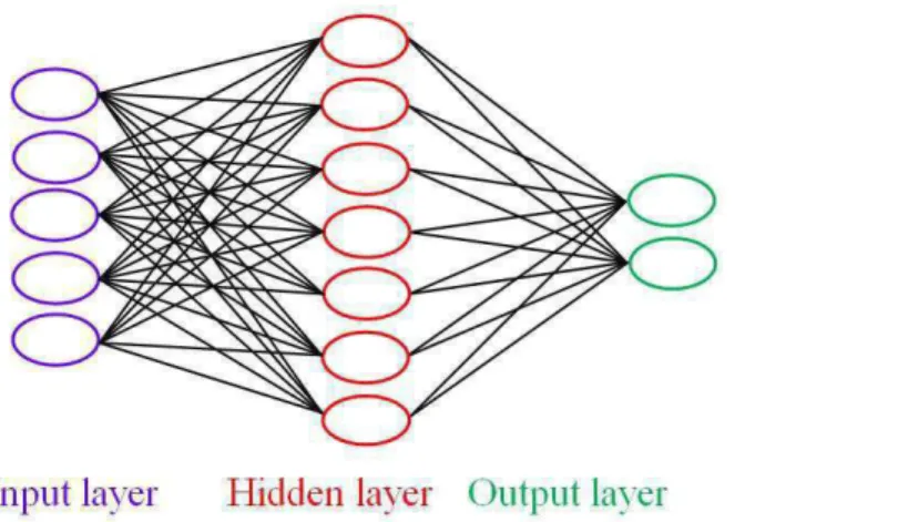
Figure 1.2: Structure of a Multilayer Perception Neural Network (MLPNN) model. ... 38
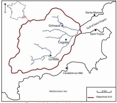
Figure 2.1: Location of the catchment. ... 4
Figure 2.2: Examples of (a) Forest, (b) Vineyard, (c) Grassland , (d) Urban area, (e) Sub-urban area. ... 6
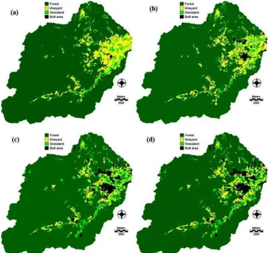
Figure 2.3 : Land cover maps of (a) 1950, (b) 1982, (c) 2008, (d) 2011. ... 9
Figure 2.4: Forest change in 1950-2008 ... 15
Figure 2.5: Vineyard change in 1950-2008 ... 15
Figure 2.6: Grassland change in 1950-2008 ... 16
Figure 2.7: Built area change in 1950-2008 ... 16
Figure 2.8: Land cover changes with altitude in (a) 1950-1982, (b) 1982-2008, (c) Forest, (d) Vineyard, (e) Grassland, and (f) Built area. ... 18
Figure 2.9: Land cover changes with slope in (a) 1950-1982, (b) 1982-2008, (c) Forest, (d) Vineyard, (e) Grassland, and (f) Built area. ... 20
Figure 2.10: Land cover changes with distance from streams in (a) 1950-1982, (b) 1982-2008, (c) Forest, (d) Vineyard, (e) Grassland, and (f) Built area. ... 23
Figure 2.11: Land cover changes with distance from road in (a) 1950-1982, (b) 1982-2008, (c) Forest, (d) Vineyard, (e) Grassland, and (f) Built area. ... 24
Figure 2.12: Land cover changes with distance from built area in (a) 1950-1982, (b) 1982-2008, (c) Forest, (d) Vineyard, (e) Grassland, and (f) Built area. ... 26
Figure 2.13: Land cover changes with distance from sea in (a) 1950-1982, (b) 1982-2008, (c) Forest, (d) Vineyard, (e) Grassland, and (f) Built area. ... 28
Figure 2.14: Clearing and terracing of foothills for vineyard. ... 32
Figure 2.15: Flooding in vineyard close to stream channel. ... 32
Figure 3.1: Location of the catchment. ... 38
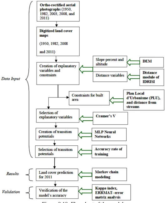
Figure 3.2: Flowchart of the model ... 39
Figure 3.3: PLU and SCOT map of the study area. ... 41
Figure 3.4: (a) Land cover map of 1950, (b) 1982, and (c) 2003, and (d) 2008. ... 47
Figure 3.5: (a) Forest change in 1950-2011. (b) Vineyard change in 1950-2011. (c) Grassland change in 1950-2011 (d) Built area change in 1950-2011. ... 48
xiv Figure 3.7: (a) Slope. (b) Altitude. (c) Distance from road. (d) Distance from built area. (e) Distance from streams. ... 50 Figure 3.8: (a) Transition potential from vineyard to forest. (b) Transition potential from grassland to forest. (c) Transition potential from forest to vineyard. (d) Transition potential from grassland to vineyard. (e) Transition potential from forest to grassland. (f) Transition potential from vineyard to grassland. (g) Transition potential from forest to built area. (h) Transition potential from vineyard to built area. (i) Transition potential from Grassland to built area. ... 54 Figure 3.9: (a) Predicted land cover map of 2011 from transition potentials 1950-1982. (b) Predicted land cover map of 2011 from transition potentials 1982-2003. (c) Predicted land cover map of 2011 from transition potentials 2003-2008. (d) Land cover map 2011 (actual) ... 58 Figure 4.1: Location of the catchment ... 72 Figure 4.2: Land cover map of 1950 (a), 1982(b), 2003 (c), and 2011(d) ... 79 Figures 4.3: (a) Observed change in different time intervals, (b) intensity of different time intervals ... 81 Figures 4.4: Gross gains and losses in 1950-1982 (a) and gain and loss intensity in 1950-1982 (b) ... 82 Figure 4.5: Gross gains and losses in 1982-2003 (a) and gain and loss intensity in 1982-2003 (b) ... 83 Figure 4.6: Gross gains and losses in 2003-2011 (a) and gain and loss intensity in 2003-2011 (b) ... 84 Figure 4.7: Transition area to vineyard in 1950-1982 (a), annual transition intensity to vineyard in 1950-1982 (b) ... 85 Figure 4.8: Transition area to vineyard in 1982-2003 (a), annual transition intensity to vineyard in 1982-2003 (b) ... 86 Figure 4.9: Transition area to vineyard in 2003-2011 (a), annual transition intensity to vineyard in 2003-2011 (b) ... 86 Figure 4.10: Transition area from vineyard in 1950-1982 (a), Annual transition intensity from vineyard in 1950-1982 (b). ... 87 Figure 4.11: Transition area from vineyard in 1982-2003 (a), Annual transition intensity from vineyard in 1982-2003 (b) ... 88 Figure 4.12: Transition area from vineyard in 2003-2011 (a), Annual transition intensity from vineyard in 2003-2011 (b) ... 88 Figure 4.13: Disagreement values according to spatial extent and cell size for 25 m, 50, and 100 m cells sizes ... 91 Figure 4.14: Disagreement values for upscaling / downscaling effects for 25 m, 50-25 m, and 100-25 m. ... 93 Figure 5.1: Vineyard affected by heavy rainfall (Photos: D. Fox) ... 111
xv
Figure 5.2: Vineyard changes in the study area in 1950-2025 (predicted) ... 114
Figure 5.3: a) K factor and b) P factor for 2011 ... 115
Figure 5.4: Mean and median slope values for different years ... 116
Figure 5.5: Mean and median slope length values for different years ... 117
Figure 5.6: Terraced and non-terraced vineyard area in different years ... 118
Figure 5.7: Erosion rate (t/ha/yr) in different years. ... 119
Figure 5.8: a) Area of soil erosion classes in different year, b) % of vineyard in different erosion classes. ... 119
Figure 5.9: a) soil erosion map for 1950, b) soil erosion map for 1982 c) soil erosion map for 2003, d) soil erosion map for 2011, and e) soil erosion map for 2025. ... 121
1
GENERAL INTRODUCTION
PURPOSE OF THE STUDY
The issue of land cover change has become important throughout the world in recent years, not only for researchers, but also for urban planners and environmentalists advocating and planning for sustainable land use in the future. In Mediterranean Europe, land cover patterns have changed greatly since the Second World War due to intensive human activities, population growth, and urban sprawl. The rapid growth in industrial and tourism activities has accelerated land cover changes in the Mediterranean coastal area in particular. Moreover, in recent decades, urban population growth and expansion of tourism have occurred more in the French Mediterranean coastal area than the average for European Mediterranean coastal areas (Blue Plan Papers, 2001). The increasing number of secondary homes and sport harbors along the Mediterranean coastline of southeast France—“La Côte d’Azur” (the French Riviera)—has transformed the pattern of land cover in the French Mediterranean coastal area (Benoit and Comeau 2005, EAA 2011). French Mediterranean cities have become popular destinations for affluent people from France and other countries to buy vacation and retirement properties. This has resulted in significant land cover change in this region, yet very few studies describing land cover change in this particular area have been conducted to date.
Most of the previous studies on land cover change in the Mediterranean area have highlighted one particular issue and/or described one specific type of land cover change. Few studies have taken into account multiple changes concurrently. In addition, spatial patterns of land cover change and identification of driver variables influencing change have sometimes been considered, but these studies have focused mainly on altitude and slope. For example, Fox et al. (2012) analyzed the impact of land cover change on total runoff between 1950 and 2003 in the upper part of the study catchment area. They noted a small increase in runoff due to a complex pattern of land cover change, but much of the lower alluvial plain, where most changes have occurred, was ignored, and spatial controls on these changes were not examined.
At the outset of this study, 27 recent studies involving land cover change analysis and modeling using CA-Markov and Multi-Layer Perceptron (MLP) with multiple land covers and
2 urban areas were examined. No studies were found on the comparison of different time scale simulations and the impact of historical time period on land cover prediction using different time scales. Thus, in this study, land cover change has been predicted using different time scales to assess the impacts of historical time period in predicting the land cover map of 2025.
Spatial extent refers to the overall size of a particular area (Turner et al., 1989, Qui & Wu, 1996, Wu, 2004). The review of 27 recent studies (2001-2014) using CA-Markov and MLPNN modeling tools reveals that spatial extent ranged from 114.4 km² to 20,000 km², with mean and median values of 3,056.3 km² and 1,200 km², respectively. If land cover change is distributed homogeneously throughout space, then spatial extent probably has little impact on model prediction outcome. However, many areas have cores of evolving land covers surrounded by less active categories. Increasing spatial extent can introduce new land cover change dynamics (Kok & Veldkamp, 2001) or land cover categories (Turner et al., 1989), but in this study, larger spatial extent will be considered synonymous with increasing the proportional area occupied by a relatively dormant category.
Dietzel & Clarke (2004) proposed guidelines for urban simulation models on spatial resolution (10 m to 1,000 m) in four spatial extents, and found that finer resolutions of less than
parcel size (≤ 10 m) in land cover simulation may increase error by creating small and false
changes. This lower limit is well below the most frequently used 30 m resolution. At the upper limit, Chen & Pontius (2011) showed that predicted built area accuracy increased with increasing spatial resolution from 30 m to 1,920 m. Moreover, the explanatory power of driving variables can also increase with coarsening spatial resolutions (minimum resolution was 15 km²) (Kok & Veldkamp, 2001). Geri et al. (2011) found that the model’s performance increased to a perfect level of agreement with increasing cell size. Spatial extent and cell size may affect the analysis of spatial patterns of land cover change separately or together (Wu, 2004). However, few studies found tested the influence of these parameters in identifying the best cell size and spatial extent for a catchment level land cover change simulation.
Land cover change has a significant impact on land degradation including soil erosion. The Mediterranean area experiences high storm intensity on dry soil in summer and autumn; at this time, vineyard areas remain almost bare and a high rate of erosion can occur (Blavet et al. 2009,
3 Wainwright 1996, Ramos and Martínez-Casasnovas 2006). Mechanical tillage, chemical weeding, and intensive use of pesticides are the most common practices in vineyard cultivation systems in the Mediterranean area, in which soil remains bare during the whole year (Novara et al. 2011, Salome et al. 2014). These practices may result in higher crop yield and better quality grapes, but soil in these vineyards is particularly vulnerable to erosion, depletion of organic matter, chemical pollution, and loss of biodiversity (Coulouma et al. 2006, Raclot et al. 2009). Several studies found a high rate of soil erosion during the storm season (Martínez-Casasnovas et al. 2005, Wainwright 1996). Most of the studies dealing with the prediction of soil erosion focus on croplands elsewhere in the world, whereas vineyards in the French Mediterranean area have been much less studied.
STATEMENT OF PROBLEM
The principal aim of this thesis is to predict long-term soil erosion evolution in a Mediterranean context of rapid urban growth and land cover change at the catchment scale.
To achieve this, the following three specific objectives were formulated:
1. To identify the spatial dynamics of land cover change patterns in a Mediterranean catchment, namely the Giscle catchment in Southeastern France.
2. To determine the impact of temporal scales, spatial extent, and cell size on land use and land cover change (LUCC) modeling to predict land cover change accurately.
3. To determine past soil erosion patterns (1950, 1982, 2003, 2011) and predict them for the future (2025) based on projected land cover for 2025.
ORGANIZATION OF THE THESIS
This dissertation consists of seven parts, including four chapters of original research. This introductory section outlines the motivations for and goals of the study, as well as the methods of investigation. The first chapter presents a literature review of previous studies dealing with related research topics. The next four chapters of this thesis present new research findings from this study. The dissertation concludes with a final section providing a synthesis of the findings, a
4 discussion of the limitations of this study, and suggestions for future research. These are summarized below:
- Chapter 1 presents an extensive literature review covering previous academic studies on land cover change dynamics and land cover change modeling. These studies come from every corner of the world and date from 1994 to 2014.
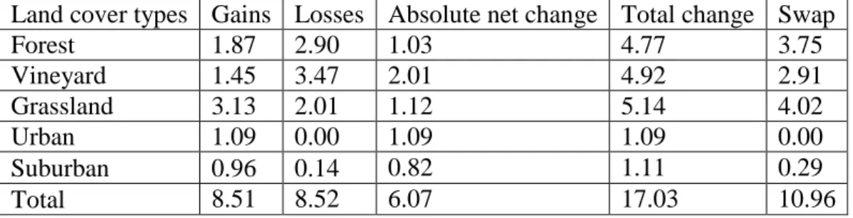
- Chapter 2 analyzes the land cover change patterns in the study area, and identifies explanatory variables for land cover change modeling by quantifying the impacts of topographic and distance variables on land cover change for each land cover category. Land cover maps were screen digitized from digital orthorectified aerial photographs. Surfaces were classified into five categories based on visual interpretation: forest, grassland, vineyards, urban, and suburban areas. Land cover change was quantified using the cross tabulation matrix of the CROSSTAB module and the Change Analysis module of the Land Change Modeler (LCM) of IDRISI Selva version 17.02 (Eastman 2012). After creating land cover maps of 1950, 1982, and 2008, land cover changes in three temporal periods were investigated: 1950-1982, 1982-2008, and 1950-2008. The land cover change determining method proposed by Pontius et al. (2004) was applied for all temporal periods to quantify persistence, gains, losses, total change (addition of gains and losses), net change, and swapping. Then, the impact of spatial variables such as altitude, slope, distances from roads, streams, sea, and built area are presented.
- Chapter 3 deals with the impact of temporal scales on land cover change modeling. Land cover maps of 2011 were predicted from different time scales (1950-1982, 1982-2003, and 2003-2008) using the Land Change Modeler (LCM), and compared with the digitized land cover map of 2011
to measure the model’s accuracy. Spatial variables - namely, altitude, slope, and distances from
roads, streams, and built area were used in land cover prediction. These variables were tested
using Cramer’s V coefficient, and identified according to the analysis in Chapter 2. Topographic
explanatory variables with several spatial and planning components were used to simulate land cover change without taking into account any particular spatial agent. Therefore, an agent-based modeling approach was not appropriate. The MLPNN-Markov model option of LCM-IDRISI, which was originally designed for land cover change evaluation and managing impact on
5 biodiversity, was used to simulate temporal and spatial patterns of change in land cover for both short and long time periods.
- Chapter 4 tests the impact of spatial extent and cell size on the perception of land cover change dynamics and land cover prediction. Spatial extent and cell size are interrelated. They can have a great impact, not only on land cover prediction, but also on perceived quality of the prediction, since calculated agreement/disagreement statistics depend on the number of cells present in the study area grid, and this depends directly on cell size and spatial extent. Change dynamics in terms of absolute and relative change were first analyzed using intensity analysis, and then land cover was predicted for 2011 for large (79.1 km²) and small (36.6 km²) windows using cell sizes of 25 m, 50 m, and 100 m. Spatial resolution effects were also analyzed by upscaling from 25 m to 50 m and 100 m and then downscaling back to 25 m.
- Chapter 5 measures the degree of soil erosion, identifies the impacts of land cover changes on soil erosion, and predicts soil erosion in vineyards for 2025 at the catchment scale using RUSLE. Chapter 3 and 4 are essential steps towards identifying the parameters for predicting land cover for the future (2025) and to see how land cover change impacts on soil erosion. Different parameters were measured. The rainfall erosion index (R) was estimated from average rainfall in the 1975-2005 period following Torri et al. (2006). The soil erodability factor K was calculated following the equation proposed by Wischmeier and Smith (1978). Based on previous studies, a cover management factor of 0.3 was used on different land cover types and vineyards conservation practice factor P is valued at 0.7 except terraces. According to field studies in the catchment area, terraces are found in most of the vineyards at slopes above 10%. Therefore, vineyards at all slopes above 10% are considered as terraced and valued at 0.2, because terraces reduce erosion by more than 50%. Soil erosion maps were predicted for 1950, 1982, 2003, 2011, and 2025. Predicted soil erosion maps were simplified into three categories: low (<10 t/ha), medium (10-25 t/ha), and high (>25 t/ha) soil erosion, respectively. For estimated erosion rates in 2025, transition potential maps were created for all possible transitions based on actual historical changes during the 1982-2003 period and explanatory variables using the MLPNN algorithm of IDRISI (Eastman, 2012). However, only transition potentials with an accuracy rate greater than 70% were included in land cover prediction, since that approach yielded better final results than
6 one which included all potential transitions. Accuracy rates greater than 70% consisted of the following: forest to vineyard, forest to grassland, forest to built area, vineyard to built area and grassland to built area. Validation values were weaker when all transitions were included, but the trends with regards to spatial extent and cell size were consistent.
7
CHAPTER 1
LITERATURE REVIEW ON LAND COVER CHANGE
DYNAMICS AND LAND COVER CHANGE MODELING
1. Land cover change
Land cover is the physical and biological cover over the surface of the land including water, vegetation, bare soil, and manmade structures (Ellis, 2011). Land use is a more complicated term that refers to the human activities such as agriculture, forestry, building construction and any other function that alters the land surface or land cover. Land cover is determined by the interaction between human activities and environmental factors such as soil characteristics, climate, topography, and vegetation.
Land cover changes are among the most important human alterations of the Earth’s land
surface (Lambin et al. 2001) and land cover conversion processes have accelerated since the Second World War (Antrop 2005, Geri et al. 2010, Serra et al. 2008). Moreover, land cover patterns of Mediterranean Europe have changed a lot since the Second World War (Fox et al. 2012) due to intensive human activities (Geri et al. 2010). Land cover change has occurred by the interaction of environmental (physical) and human (socio-economic) characteristics: population growth, urban sprawl, industrial development, and political and environmental policy. In addition, rapid expansion of industrial and tourism activities during the last six decades has caused important socioeconomic changes in rural areas of the Mediterranean area (Dunjó et al. 2003). According to Geri et al. (2011), land cover in Mediterranean areas has been changed by socio-economic development such as industrial and urban activities since the 1940s. Land use / cover change (LUCC) has a great influence on the current global change phenomena in both physical and human environments. It affects world bio-diversity and ecosystems, food security, human health, urbanization, and global climate change (Falcucci et al. 2007, Geri et al. 2011), Sala et al. 2000). It is also responsible for environmental change, water pollution and soil degradation (Dunjó et al. 2003). LUCC has resulted in the abandonment of marginal hillside
8 terraces and has shifted farm cultivation to better soils to increase profits. Three common major land cover changes in the Mediterranean area are the following: the expansion of tourism along the coastline that results in rapid urbanization, intensification of agriculture on alluvial plains and low lands, and abandonment of agricultural terraced land in mountainous steep slopes leading to their transformation to forest area (Falcucci et al. 2007).
Antrop (2005) conducted a study on landscape dynamics in Europe and divided three periods of time to show historical landscape changes in Europe: pre 18th century, 19th century to the Second World War, and post-World War II. According to the study, traditional landscape changes occurred in the first period but many new landscapes were generated upon the traditional ones in the second period. Urbanization and globalization were identified as effective factors of landscape change in the post war period. In Antrop’s (2005) study, landscape was defined as natural, rural, and urban area and characterized by the interaction of natural and human factors. Several driving forces of landscape change in Europe such as accessibility, urbanization, globalization and the impact of calamities were also discussed in the study, but not all of these driving forces are common in the Mediterranean area. Antrop (2005) also mentioned that population growth and technological advantages were associated with urbanization.
1.1 Major trends in Euro-Mediterranean land cover change
Land cover changed greatly in the Mediterranean coastal area after the Second World War because of the industrial and agricultural revolutions. Slope and elevation, soil conditions, and other environmental factors were taken into consideration by farmers in the first part of the 19th century to establish agricultural farms, but this changed after the Second World War when human factors became more influential than environmental factors for land cover change because of high demographic pressure and socio-economic development in the Mediterranean area. Urbanization increased rapidly along the coastline, with resident population doubling every 30 years and tourism every 15 years (Falcucci et al. 2007).
According to different studies (Geri et al. 2011, Nunes et al. 2011), two general trends of land cover change took place in recent decades in the coastal Mediterranean area. Firstly, dry farming
9 and forest land cover decreased in alluvial plains while reforestation occurred in hilly area. Secondly, urbanization occurred rapidly in most of the coastal plains where the tourism industry flourished. Development of infrastructure, communication networks, and technological advances resulted in socio-economic development that was the main reason for agricultural land abandonment on marginal lands. Population growth and socio-economic development caused agricultural intensification that increased irrigated crops. Different studies have been carried out to identify the factors and spatial patterns of land cover at various scales (Kok and Veldkamp 2001, Verburg et al. 1999). According to Serra et al. (2008), the expansion of tourism in the coastal Mediterranean area, environmental protection of certain areas, and common agricultural policy in Alt Empordà county (north west of Catalonia, Spain), caused important land cover changes in 1977-1997: “Agrarian abandonment has caused the depopulation of inland hill and
mountain areas, whereas tourist activities have resulted in substantial population increases along the coastal zone” (Serra et al. 2008).
In the 1960s, agricultural activities were influenced by natural climatic conditions, such as rainfall. About 50% of the total agricultural area in Portugal was utilized for non-irrigated cereal cultivation (sown between October to November to make use of precipitation) and unseeded fallow rotation (Nunes et al. 2011). But the scenario changed in the latter half of the 20th century; agricultural activities became less important in the Mediterranean area due to natural barriers: relief and uneven topography, poor soil quality, and uncompetitive farm structures such as small,
scattered plots. “Nowadays, shrub land cover and vine and olive tree patches are the most typical vegetation of the physiognomy and ecology of Mediterranean environments, leading to a whole homogeneous landscape and the consequent loss of biodiversity” (Dunjó et al. 2003).
Fox et al. (2012) conducted a study to analyze the impact of land cover change on total runoff in a Mediterranean catchment between 1950 and 2003 in the context of river management. Factors and patterns of land cover change were also explained briefly in the study. According to the study, land cover of the study area is strongly influenced by topography and most of the land cover changes occurred in the alluvial plain and foothills (about 29% of the catchment). Forest occupied about 90% of the gauged catchment and most of this was situated in upper hilly area. Vineyards and grassed areas covered the most area after forest and had a high tendency to
10 transform into urban areas. Some forested area also converted to vineyard in the study period but it was less than the area transformed from vineyard to forest.
Falcucci et al. (2007) measured land cover changes in the Italian peninsula between 1960 and 2000. According to the study, land cover/use changes occurred all over the Italian peninsula, particularly in Apennines and Mediterranean coastal areas from 1960s. Forest area roughly doubled in the Alps and Apennines as it gained land from agricultural areas. Agriculture area decreased in hilly and coastal areas but expanded in the rest of the country where traditional cultivation was transformed to modern technology based intensive cultivation. Land cover change was also related to population density which increased in plains and coastal areas because of tourism, agriculture and urbanization.
Geri et al. (2010) analyzed land cover change in a Mediterranean catchment (Siena province, Italy) in 1954-2000. They observed the direction and rate of land cover change and focused on the effects of human activity/disturbance in a Mediterranean environment. Forest and agricultural areas were more stable whereas semi natural areas were unstable in their study area. About 6% forest cover changed to agricultural land, and 12% and 3.5% of crop land converted to forest and semi natural area, respectively. But 55% and 35% of semi natural area transformed to forest and agricultural area, respectively. The study revealed that losses of forest area occurred mainly at higher elevations and conversion of agricultural land (both crop land and semi natural) occurred at lower altitudes.
Sluiter and de Jong (2007) conducted a study on land cover change in Peyne, France. According to the study, intensification of vineyards increased due to the expansion of the worldwide wine market and on automatic harvesting system. They found that about 90% of land abandonment occurred before 1940s, and was located further away from urban areas and roads. They also mention that intensification and modernization of agriculture were major factors of such change at the time of the “Green revolution”. Recent abandoned agricultural areas were near urban areas because most of recent abandonment occurred due to urban sprawl and industrialization.
11 Alemayehu et al. (2006) analyzed land cover change in the context of demographic desertification in Tabernas (Almeria, Spain) and the study area represented a Mediterranean region where a combination of extreme environmental and land cover changes occurred in the last decades. The study showed that 32 % (2,507 ha) of dry farming areas were changed into different land cover types in 1956-2000, of which 57.7% (1,447.7 ha) changed to irrigated farmland (twice the irrigated area in 1956), 34% (857 ha) were abandoned, and about 8.3% (202 ha) changed to urban and industrial development structures. The study also revealed that land abandonment and the transformation of dry farming land to irrigated crops increased soil erosion, salinization and pollution.
Cori (1999) explained that rapid growth of the tourism industry increased dramatically in the last few decades and influenced land cover change on the northern shores of the Mediterranean area. According to the study, rapid growth of population, tourism activities, change of settlement system, and industrial development were the main causes of land cover change. It was reported that agricultural land decreased and non-agricultural land increased in the Spanish, French, and Italian Mediterranean regions. It also demonstrated that the agricultural areas were affected due to the spread of tourism and traffic infrastructure such as urban structure, hotels, roads etc. In the study, several spatial planning policies were discussed and new plans were introduced to conserve the Mediterranean environment, particularly in Spain, France and Italy.
Van Eetvelde and Antrop (2004) analyzed the characteristics and mechanism of land cover change in southern France (Tavernes) in 1960-1999. They explained how structural and functional changes influenced new landscape formation in their study area. They also identified three main trends of land cover change in Mediterranean areas: development of transportation and infrastructure, urban sprawl, and rapid expansion of the tourism industry in the Mediterranean coastal area. According to the study, little land cover change occurred in the Tavernes basin in 1979-1993. A particular pattern of transition was noticed from vineyards to olive groves. Most of the changes occurred on the foot slopes in the northern and eastern edge of the basin.
Serra et al. (2008) reported that mass tourism on the coast, the development of irrigation projects, environmental reserve areas and common agricultural policy (CAP) subsidies for
12 irrigated crops were the main causes behind land cover and land cover changes in the Mediterranean area. They revealed that irrigated maize, fruit trees, shrub lands, deciduous forest, and urban areas increased significantly in coastal plain areas. Besides, vineyards and olive trees decreased in the mountainous areas and transitional sub regions that resulted in land abandonment and increased shrub land area.
Koulouri and Giourga (2007) conducted a study in Lesvos Island, Greece. They considered
three land cover “types” such as cultivation, short-time abandonment, and long-time
abandonment to describe the relationship of land abandonment and soil erosion that occurred by the changes in agricultural practices and soil resource management. Significant land cover change occurred on steep slopes (≥ 25 %). The study revealed that soil erosion increased significantly on
steep (≥ 25 %) to very steep slopes (≥ 40 %) because of loss of densely protective plant cover and
increase in shrub cover. In addition, increased bare soil area was also described as another major cause of soil erosion.
1.2 Factors affecting land cover change
Land cover change occurs under the pressure of a variety of socio-economic factors that interact with the natural environment to determine the nature and location of land cover change. The list below is not exhaustive but lists the major factors currently referred to in the scientific literature for the Mediterranean area.
1.2.1 Demographic pressure and urban sprawl
Population growth and urbanization have occurred in Mediterranean coastal areas as in other parts of the world. About 60% of the world’s population resides in a 65 km wide belt close to the coastline because of its beauty, natural resources and economic activities (Vallega, 1998). Urbanization is a major driving force of land cover change, though it occupies a very small
fraction of the Earth’s land surface (less than 2%). About 51 % of the world’s population were
13 will be living in urban areas by 2030 (UNFPA 2004). Urbanization affects urban fringe areas which are progressively transformed into full urban areas. Brauch (2003) estimates that the population of Southern European countries doubled in 1950-2000, and the urbanization rate has been projected to increase from 44.2 % in 1950 to 75.2% by 2030; in addition, urban population will reach 71.6 % in Greece, 76.1% Italy, 81.6 %, in Portugal, 82.2 %, in France, and 84.5 % in Spain by 2030, respectively. In Southern Europe, the population of some major Mediterranean coastal cities (Athens, Barcelona, Naples, and Marseille) increased 1.1 to 1.8 fold from 1950 to 2000 and should stabilize around 2015.
The population density in the Mediterranean coastal area (69 inhabitants/km2) is more than double the density of population of the region as a whole (47 inhabitants/km2) (Benoit 2001, Cori 1999). According to Benoit (2001), Mediterranean coastal regions are more urbanized than countries as a whole, and urban and total population in Mediterranean area increased by 2.7 and 1.9 times, respectively, in 1950-1995. Total population growth rates in 1950-1995 were 0.54% and 0.29% in France and Spain, respectively, but population growth rates in Mediterranean coastal regions of these countries were 0.76% and 0.49%, respectively. According to Falcucci et al. (2007), a decrease in population was observed in the Apennines, Alps, and in the central and mountainous part of Sicily and Sardina of Italy in 1960-2000 while an increase was noted along the coastal areas due to rapid growth of economic activities.
Urbanization is a continuous process that was initiated in Europe during the industrial revolution in the nineteenth century (Antrop 2005). Socio-economic development and population growth were two main factors behind it. In Mediterranean Europe, many large cities experienced strong growth rates between the 1950s and the 1980s (Catalán et al., 2008). However, the presence of many small and medium-sized urban centers near large cities contributed to knit together metropolitan regions (Benoit, 2001). For example, urban sprawl is growing rapidly in the Mediterranean area, as in Madrid, Marseilles, and some other cities of southern Europe. According to Benoit (2001), the European Mediterranean coast is now almost completely urbanized where average distance between urban areas was about 10 km, 17 km, and 18 km in Italy, Spain, and France, respectively, in 1995. Moreover, the number of urban areas also increased dramatically in the European Mediterranean basin in 1950-1995 (Benoit, 2001). The
14 number of urban areas was 296, 676, and 350 in France, Italy, and Spain, respectively, in 1950, and increased to 433, 769, and 415, respectively, in 1995. Urban growth expanded along the periphery at the expense of agricultural or forest areas.
According to Benoit and Comeau (2005) Mediterranean countries from Spain to Greece experienced strong urban growth until the 1970s, and their current moderate growth rates are projected to continue. Land cover change has been affected by newly developed artificial areas: for example, total built area, roads & car parks, and non-built artificial area (gardens, lawns and construction sites) increased by 12%, 10%, and 17%, respectively, in France between 1992 and 2000 (Benoit and Comeau, 2005). About 34% of Spanish Mediterranean coastal areas have been urbanized since 1999 and this figure was 43% for the Italian coastline (Serra et al. 2008). As a result, only 4.7% of primary vegetation in Mediterranean Europe remains unchanged (Geri et al. 2010). In addition, migration from other European countries tends to concentrate in the Mediterranean coastline area due to the quality of life in Mediterranean cities (Cori 1999). Aging population in Europe has a typical migration trend towards the Mediterranean coastal zone (Van Eetvelde and Antrop 2004).
1.2.2 Tourism
The Mediterranean is the world’s leading tourist destination where tourism is a major industry
in terms of economic activity (MAP 2008), and tourism is one of the most important sources of income for most Mediterranean countries. Though tourists tend to visit mainly in summer, infrastructures such as housing, roads, and entertainment facilities are built permanently, contributing to accelerate urban growth. According to Enne et al. (2005), the Mediterranean region attracts more than 30% of world tourism. Benoit (2001) predicts an average 250 million visitors per year for 2025 in Euro-Mediterranean coastal areas. According to the report of MAP (2008), the number of tourists in the Mediterranean coastal area will increase by about 80% between 2000 and 2025.
Significant human pressure on the Mediterranean coast is caused by the expansion of tourism related to seaside resorts. Van Eetvelde and Antrop (2004) explain that natural, cultural and
15 scenic values of Mediterranean landscapes were important factors for developing the tourism sector, and new infrastructure developments based on tourism have changed the traditional form of land cover and socio-economic conditions. France received 60 million tourists in 1996 and over 80 million 2007, representing almost 11% of world tourism at the time (Wikipédia, http://fr.wikipedia.org/wiki/Tourisme_en_France). France is the first tourist destination in the world with the third highest income from tourism (after the U.S.A. and Spain). In addition, the World Tourism Organization (WTO) predicted about 100 million foreign tourists will visit France in 2015. Every year, millions of tourists gather in summer in coastal cities to enjoy the Mediterranean Sea and the rugged topography of the Southern Alps, because the dominant climatic regime is typically Southern Mediterranean with mild winters and dry summers. Mediterranean France has a very rich mixed environment, and it presents many of the typical features of Mediterranean tourism, especially in coastal areas, where strong urban development is related to tourism.
According to Cori (1999), Mediterranean countries provide at least 25% of the world’s hotel accommodation. Coastal regions of other Mediterranean countries such as Turkey, Cyprus, and Morocco have also been influenced by expansion of the tourism industry. These coastal areas are more urbanized due to the rapid development of local tourism. Greece and Croatia are the leading countries in northeastern Mediterranean with their high potentialities to attract international tourism. Greece has the combined appeal of its archeological and artistic heritage with the traditional sea-sun-shore. The expansion of tourism on the coastal plains and even in the inner mountainous forest areas has reduced the natural and cultural biodiversity, and the degradation of former traditional agricultural landscapes has increased forest fires and soil erosion (Serra et al. 2008).
As described by EAA (2011), the number of secondary homes increased by 10% between 1990 and 1999 in France, creating intensive pressure on the environment, especially in coastal and mountain zones. There is a sport harbor every 3 km and most of these harbors are accompanied by urban development operations in the Mediterranean coastline of southeast France - “La Côte d’Azur” (Benoit 2001, EAA 2011). According to the report of EAA (2011), almost 335,000 new secondary homes were built during the past two decades, occupying 22 km²
16 of land. In the 1990s, Mediterranean beaches attracted people of central and Eastern Europe as well as the inland population from the Southern side of the Mediterranean basin (Benoit 2001), and both domestic and external tourism are increasing. Moreover, retired population from home and abroad (many from Northern Europe, and African and Arabian elites) have a tendency to buy property and houses in a Mediterranean city. According to (Cori 1999), half of total secondary homes in France are situated in the Mediterranean coastal area.
1.2.3 Intensification of agriculture
Fine grained rural landscape structures are being replaced by large scale ones leading to loss of regional diverse cultural landscapes due to the intensification of agriculture (Van Eetvelde and Antrop 2004). Intensive agriculture can be defined as a cultivation system that uses high input such as labor, fertilizer, pesticides, herbicides, fungicides and capital to obtain maximum yield per unit of land (Lambin et al. 2001). Intensive agriculture requires less land area than extensive agricultural farms but it needs high efficiency machinery for planting, cultivating, harvesting, and producing a similar profit. Generally, farmers use greater farm areas in intensive cultivation for sustainable use of their capital investments and equipment to get higher profit. Nowadays, this type of agriculture is practiced throughout the developed world to increase food production for a rising population. But the pattern of agricultural landscape has changed in Europe since the Second World War because of agricultural and economic development (Geri et al. 2011). Modern intensive agricultural practices ensure food security, increased income, and improved farmer’s living standards in both developed and developing countries. The intensification of agriculture occurred mainly based on technological advances and improvements in agricultural materials and machinery, and it has reduced corresponding production costs. Optimum use of organic and chemical fertilizer, development of irrigation, and practice of advance technology in agriculture and animal husbandry increased productivity of land and crop yields per unit area. The “Agri-Basin” of Italy has experienced the relocation of profitable agricultural activities from uplands to plains due to rapid intensification in agriculture (Quaranta, et al. 2001). In addition, profitable
17 crops such as high yielding varieties are cultivated over huge areas due to increased investment in irrigation.
Two patterns of agricultural land cover change in European Mediterranean areas over the last fifty years can be defined (Baldock et al. 1996).
Suitable and more productive land cover was converted to more intensive agricultural uses
since the 1950s, often with an expansion of arable land at the expense of permanent grassland, wetlands, and forest.
Marginal areas with physical and socio-economic barriers such as steep slopes, small
terraces, wet areas without drainage systems, and remote mountain regions have been abandoned or replaced by specialized farming systems, plantation forestry or natural succession.
1.2.4 Land abandonment
“Land abandonment can be defined both qualitatively (as a description of the land condition) and quantitatively (as years without use)” (Moravec and Zemeckis 2007). The concept of
land/farm abandonment is applied to the land where traditional or recent agricultural use has stopped. There is no well-defined and commonly accepted definition for land abandonment
because there is confusion over the term “abandoned farmland”. Sometimes apparently
abandoned land often is not truly abandoned, but merely temporarily out of use/cultivation and awaiting a new owner or tenant. In the European Mediterranean, legal owners of much of the abandoned farmland live in a town or city, and they bought their farmland as an investment. The statistical survey of France separates abandoned land from fellow land, but there is no specified duration when fallow land converts to abandoned land (Moravec and Zemeckis 2007).
Dunjó et al. (2003) described the land abandonment process in a typical Mediterranean environment (North East Spain) during the last century. They divided four different land cover types according to the duration of land abandonment such as cultivated fields (vineyard and olive trees, 0 years), recent abandonment (densely and cleared shrubs, 5 years), mid-abandonment
18 (cleared cork trees and dense olive trees, 25 years) and early abandonment. Most of the studies (Geri et al. 2010, Koulouri and Giourga 2007, Sluiter and de Jong 2007, Van Eetvelde and Antrop 2004) about land abandonment in Mediterranean Europe show that mountainous or semi mountainous hillside areas were abandoned because small plots of vineyards and olive trees were not profitable. Land abandonment is also a common scenario in Mediterranean France because of technological, social, and economic change (Geri et al. 2010, Sluiter and de Jong 2007). Intensive agriculture and long term abandonment started around the 1850s and increased to a high rate after
1900 in ‘Peyne’, Southern France (Sluiter and de Jong 2007). But it is difficult to understand the
real condition or measure changes that occurred because of complex transitions between vegetation and agricultural land. Van Eetvelde and Antrop (2004) describe how land abandonment and urbanization have been occurring simultaneously in their study areas - Tavernes, le Flexi and Montfaucon of southern France. Most of the changes took place in the last few decades because of urbanization and agricultural intensification.
There are different causes of agricultural land abandonment and according to Baldock et al. (1996) and land abandonment may take place in the following ways:
Temporarily out of use
Farmland which is under irregular management or waiting a new owner or tenant may
seem abandoned.
Farmland which is converting to non-agricultural use seems abandoned, typically in urban
fringe areas.
Farmland which is temporarily set aside under the Common Agricultural Policy (CAP)
arable regime may also appear abandoned.
Permanently abandoned
Land which is under long term set aside schemes, such as habitat creation under
Regulation 2078/92 and subject to conservation management.