Blind Submarine Seismic Deconvolution
for Long Source Wavelets
Benayad Nsiri, Associate Member, IEEE, Thierry Chonavel, Jean-Marc Boucher, Senior Member, IEEE, and
Hervé Nouzé
Abstract—In seismic deconvolution, blind approaches must
be considered in situations where reflectivity sequence, source wavelet signal, and noise power level are unknown. In the presence of long source wavelets, strong interference among the reflectors contributions makes the wavelet estimation and deconvolution more complicated. In this paper, we solve this problem in a two-step approach. First, we estimate a moving average (MA) truncated version of the wavelet by means of a stochastic expec-tation–maximization (SEM) algorithm. Then, we use Prony’s method to improve the wavelet estimation accuracy by fitting an autoregressive moving average (ARMA) model with the initial truncated wavelet. Moreover, a solution to the wavelet initializa-tion problem in the SEM algorithm is also proposed. Simulainitializa-tion and real-data experiment results show the significant improve-ment brought by this approach.
Index Terms—Bernoulli–Gaussian (BG) process, blind
decon-volution, Gibbs sampler, maximum likelihood (ML), maximum posterior mode (MPM), Monte Carlo Markov chains (MCMCs) methods, Prony algorithm, seismic deconvolution, stochastic expectation–maximization (SEM).
I. INTRODUCTION
T
HE aim of marine seismic exploration is to recover the geological structure of the sea bottom lithography from the analysis of reflected acoustic waves, originating in a seismic wavelet emitted by an acoustic source. The recorded seismic trace can be modeled as the convolution between a source wavelet and a reflectivity sequence, in the presence of additive noise [1]. It is often necessary to apply an inverse transform, called deconvolution, to obtain the reflectivity sequence and Manuscript received July 10, 2006; revised March 30, 2007; accepted April 16, 2007. This work was supported by IFREMER, Bretagne Region, France.Associate Editor: R. Chapman.
B. Nsiri is with the Ain Chock Faculty of Sciences, Physics Department, University Hassan II, Casablanca 20101, Morocco, the Groupe Signaux, Communications et Multimédia, Laboratoire de Recherche en Informatique et Télécommunication (GSCM-LRIT), Rabat, Morocco, and the Ecole Nationale Supérieure des Télécommunications (ENST) de Bretagne, Brest 29200, France (e-mail:[email protected]).
T. Chonavel is with the Department of Signal and Communications, Ecole Nationale Supérieure des Télécommunications de Bretagne, Brest 29200, France (e-mail: [email protected]).
J.-M. Boucher is with the Department of Signal and Communications, Ecole Nationale Supérieure des Télécommunications de Bretagne, Brest 29200, France and the National Scientific Research Center Laboratory, Traitement Algorithmique et Matériel de la Communication, de l’Information et de la Connaissance, UMR 2872, Brest 29238, France (e-mail: jm.boucher@ enst-bretagne.fr).
H. Nouzé is with the Marine Geosciences Department, Institut Français de Recherche pour L’Exploitation de la Mer, Bretagne 29280, France (e-mail: [email protected]).
Color versions of one or more of the figures in this paper are available online at http://ieeexplore.ieee.org.
Digital Object Identifier 10.1109/JOE.2007.899408
to improve the detection accuracy of layers from seismic data records. If the source wavelet is known, reflectivity can be recovered quite easily from the seismic trace [1]. However, in marine seismic deconvolution, the source wavelet is not exactly known, at least for the following two reasons: acoustic sources such as air guns and sparkers cannot be sufficiently controlled in operational conditions, and the received signal is modified by the ghost phenomenon caused by multiple reflections on the free sea surface and high-frequency absorption during propagation. In practice, a simple way to account for these later phenomena consists in modeling them through distortion of the wavelet [2]. Then, the source wavelet is not exactly known and a blind deconvolution procedure must be applied to recover the unknown source wavelet and the reflectivity sequence [3].
If the wavelet is sufficiently short, as in high-resolution marine seismic exploration [2], where the studied seabed thickness is only about 100 m with a resolution of 1 m, blind deconvolution gives only small improvements compared to raw seismic traces. On the contrary, in some experiments, the emitted wavelet must have a very small frequency bandwidth to penetrate deeper in the soil. As a consequence, we get a long oscillating wavelet. In this case, the seismic image obtained by stacking up consecutive traces is blurred and blind deconvolu-tion is really useful in producing quality images for geologists. In such situations, estimating directly the model parameters as in [4] generally yields a high variance of the wavelet estimator. So far, many techniques have been proposed to solve the problem of blind deconvolution with respect to different criteria. They are based on the classical hypothesis of reflectivity white-ness. One early technique that copes with the presence of noise is based on Wiener filtering [1], [3]. It supplies a minimum phase wavelet from the second-order statistical content of the trace signal. Unfortunately, this approach is not satisfactory since the source wavelet is usually nonminimum phase. Thus, further sta-tistical information upon the reflectivity sequence must be con-sidered to recover the wavelet phase [5].
The sparse nature of the reflectivity sequence is not well described by a Gaussian model, as assumed when minimum-variance deconvolution [3] is applied. In addition, non-Gaussianity is mandatory for blind deconvolution of scalar signals convolved with a nonminimum phase filter. A main underlying idea in using higher order statistics is highlighting non-Gaussianity of the deconvolved sequence by maximizing contrast criteria [6], [7].
Many related solutions have been tested. In particular, wavelet spectrum envelope can be estimated by using an au-toregressive moving average (ARMA) model of the wavelet, that is, a wavelet with rational transfer function. Its phase can 0364-9059/$25.00 © 2007 IEEE
be recovered by maximizing a kurtosis criterion [8] thanks to reflections through the unit circle of zeros of the moving average (MA) part, that is, the polynomial part of the wavelet. Alternatively, multispectral techniques can be used, for in-stance, by recovering the phase of the bispectrum of the trace after it has been whitened at the second order [9].
The main difficulty of these approaches is that they require a large amount of data to achieve reliable estimation. But, in general, seismic trace signals often contain less than 1000 sam-ples, leading to limited performance with the aforementioned approaches.
Another way of applying the whiteness hypothesis for de-convolution consists in minimizing the mutual information rate [10]. It is related to the Küllback–Leibler divergence, which measures the independence degree of the deconvolved data se-quence. Unfortunately, this method is not robust with respect to additive noise level, and its performance drops as the signal-to-noise ratio (SNR) decreases.
Instead of considering higher order statistics or general pur-pose information criteria, a nice way to fully account both for non-Gaussianity and sparseness of the reflectivity sequence con-sists in considering a prior probability model for the reflectivity sequence. In [11], Mendel introduced a Bernoulli–Gaussian (BG) model of the reflectivity sequence. The Bernoulli variable indicates the presence or absence of a reflector. This model has been extended to a mixture of two Gaussian distributions by associating the high-variance Gaussian distribution to strong reflectors [4], [11]. More precisely, conditional to the value (zero or one) of the Bernoulli variable, the sequence at the point under consideration has a Gaussian distribution with either low or high variance, the later case corresponding to the presence of a reflector. Recovering this reflectivity sequence from the data and the corresponding underlying state (strong or weak reflectivity) enables layers localization in the subsurface. The direct optimization of the corresponding likelihood criterion is unfeasible in practice and many approximate solutions to this problem have been proposed. In particular, the single most likely replacement (SMLR) [11] is a suboptimal solution to this problem. It works in the following two iterative steps: 1) an estimate of the wavelet is calculated from data and an esti-mated reflectivity sequence and 2) one reflector is updated (the one that achieves best posterior likelihood increase) with this wavelet. The SMLR works in real time, but it may converge to a local optimum. The iterated window maximization algorithm [12] looks very similar to the SMLR, but instead of modifying only one variable at each step, many variables are updated at the same time, leading to improved estimator.
The posterior mean estimator of the reflectivity sequence can be found by using Monte Carlo Markov chains (MCMCs) [13], at the expense of higher computational effort.
As far as unknown parameters such as the wavelet or possibly unknown parameters of the BG model or additive noise variance are concerned, a standard tool for estimating them is the expec-tation–maximization (EM) algorithm [14], [15] that maximizes the likelihood functional of the completed data model, that is the model that accounts for hidden variables corresponding here to the reflectivity and its underlying Bernoulli process. But, due to its deterministic structure, the EM converges to a local optimum.
This problem can be overcome by using stochastic versions of the EM algorithm, namely, the stochastic EM (SEM) algorithm [16], [17] or the stochastic approximation EM (SAEM) [18]. Finally, the estimation of the BG noise and source wavelet pa-rameters can also be solved by means of MCMC techniques in a fully Bayesian framework. In this case, parameters’ prior dis-tributions are introduced [19]–[22]. A comparison of SEM and Bayesian approaches can be found in [4].
After parameter estimation, a further step is carried out to enable reflectivity sequence deconvolution. This is achieved by the maximum posterior mode (MPM) method [23], [24], which also involves MCMC simulation through Gibbs sampling [25]. Let us note that an alternative to the MPM for BG deconvolution is the closely related but suboptimal iterated conditional mode (ICM) algorithm [26].
SEM and Bayesian approaches have been applied mostly with short wavelets. Let us remark that the short wavelet case has been extended to multichannel deconvolution [27]. So far, the long wavelet case has not been considered often, despite its prac-tical interest [28]. In fact, dealing with long unknown wavelets is a difficult task. In such situations, direct ARMA modeling of the wavelet generally appears to fail and estimating the param-eters of a long MA model generally yields high variance of the wavelet estimator.
In this paper, we propose a new method to deal with long ARMA wavelet sources in reflectivity blind deconvolution that overcomes the aforementioned problems within the framework of classical blind seismic deconvolution techniques. More pre-cisely, the following two-step approach is proposed. The first step yields a robust estimation of a truncated version of the wavelet by using the maximum-likelihood (ML) approach, via an SEM algorithm. Then, an improved wavelet estimation is achieved by fitting an ARMA model with the initial wavelet trun-cated version (MA model), using Prony’s algorithm [29], [30].
In addition, we propose an efficient method to estimate the order of the initial MA wavelet, based on a tradeoff between bias and variance, and we introduce a new criterion to ensure an accurate wavelet impulse response initialization in the SEM procedure. These are important practical issues for achieving accurate wavelet estimation.
This paper is organized as follows. In Section II, we describe the data model and the standard SEM and MPM procedures for blind reflectivity deconvolution. In Section III, we describe our two-step improved wavelet estimation procedure. In Section IV, we address the problems of the initial MA wavelet order selec-tion and of its initial choice in the SEM procedure. In Secselec-tion V, we show on simulations and on real-data experiments the signif-icant improvement brought by this approach. Finally, we sum-marize our work in Section VI.
II. DATAMODEL ANDSTANDARDPROCEDURES FORBLIND REFLECTIVITYDECONVOLUTION
The blind submarine deconvolution aims at restoring the se-quence of sea bottom reflectivity. The observed signal consists of a noisy version of the reflectivity sequence convolved with the source wavelet
where is the wavelet finite-impulse response of length , is the reflectivity sequence, and is the observation white noise sequence with variance . The reflectivity process is described by means of a generalized BG process [11], characterized by an underlying
state model with at high reflectivity
points and at low reflectivity points. Thus, condi-tional to is distributed according to a zero-mean Gaussian distribution with variance if and if
(2) with being the probability of having a reflector at position , and . The BG distribution parameter
vector will be denoted by . For sake of
clarity, we recall derivations of the standard SEM and MPM procedures.
A. Maximum Likelihood
To solve the deconvolution problem, one needs to estimate . For that, we can use the log-likelihood criterion
[3]. Unfortunately, direct maximization of the log likelihood is unfeasible. However, we are confronted with an incomplete data problem [14] where the incomplete data are given by , with . Then, we are led to work with the log likelihood of the completed data model, defined
by . Since , can be
written as
(3) Each component of this equation can be expressed easily. As is a vector of independent Bernoulli variables,
. Furthermore, the vari-ables are independent conditional to the variables . Ac-cordingly
(4)
(5) where represents convolution, with
(6) and and are the convolution matrices associated with and , respectively.
B. Gibbs Sampler
When the complete data vector is known, with respect to , maximizing is straightforward [see (5)]. In practice, is unknown, but it can be simulated using the Gibbs sampler [31], which consists of an iterative random simulation according
to the probability distribution ,
where . The
moti-vation of the Gibbs sampling is that iterative drawing of
entries , , of a vector
from amounts to simulating the whole distri-butions of [31] in a generally much simpler way. Note
that , where
. The expressions
of , , and
can be found in [33].
For the simulation of , iterations of the Gibbs sampler are implemented as follows [13], [25].
For and , do the following:
• compute [see (1)];
• simulate ( denotes the
Bernoulli distribution with parameter );
• simulate ;
• update :
C. SEM Algorithm
Since we can now simulate with the Gibbs sampler, the SEM algorithm can be used to estimate . The SEM algorithm is a stochastic version of the EM where the expectation step is replaced by simulation of one variable . Starting from an initial parameter , an iteration of SEM consists of the following steps, for iterations :
• SE step: simulate ;
• M step: .
The SEM does not converge pointwise. It generates a Markov chain whose stationary distribution is more or less concentrated around the ML parameter estimator. A natural parameter esti-mate from an SEM sequence is the mean of the
it-erates value where the first burn-in
iterates have been discarded. An alternative estimate would be
the parameter , , leading to the highest
likelihood.
Leaving for clarity the iteration exponent , the SEM al-gorithm can be summarized as follows.
• Initialization: choose and . • For
— E step: simulate ;
— M step: calculate the parameters
(7)
where .
D. MPM Deconvolution
At the end of the SEM procedure, is well estimated while reflectivity is not. The fact that the wavelet is accurately
es-timated while reflectivity parameters are not can be understood easily: The wavelet estimation benefits from multiple reflectors diversity, and since it has a smooth shape, its mean square or ML estimate is little affected by reflector position small shifts or close reflectors overlapping. On the contrary, the parameters of a single reflector do not benefit from averaging effects in their es-timation. Similarly, parameters represent noise and reflectivity statistics. Thus, they also all benefit more from statistical averaging since the record is long. Therefore, an ad-ditional deconvolution procedure based on the MPM algorithm is performed for recovering from knowledge of [33].
As the parameters, and, in particular, wavelet , are com-pletely estimated by the SEM procedure, the deconvolution is no longer blind. But we still need to estimate the hidden vari-ables in vector from the observation.
To estimate , let us remark that the posterior log likelihood of conditional to and is
(8) where the function does not depend on . The principal separation [11] allows us to address the maximization of in the following two steps:
• detection: ;
• estimation: .
is quadratic in , for fixed , leading to
(9) The detection step is not so easy, because the vector has ( is the signal length) configurations. Testing all of them is not possible. Instead, the posterior mode of each individual can be searched applying for the MPM [19], [24].
The MPM algorithm simply generates samples of drawn from just as for the Gibbs sampler used in the SEM algorithm and described at the end of Section II-B. Then, from these samples , a decision is made upon each
, and is estimated conditionally to as follows. • Detect if otherwise. (10) • Estimate if otherwise. (11)
For , is the posterior mode of . Other values of correspond to other Bayesian cost functions [34].
III. IMPROVEDWAVELETESTIMATION
In some seismic experiments, the wavelet impulse response is quite long. In such cases, the mean square error (MSE) of the estimator is quite large. In particular, the last coefficients of , which have small values, are poorly estimated. For this reason, searching for a vector with reduced length generally enables a good compromise between bias and variance properties of the estimator. However, performing the MPM deconvolution with a truncated wavelet will degrade detection and estimation perfor-mance for the reflectivity sequence.
The true wavelet can be described by an MA model of length [MA model] with transfer function . To avoid using a model with many parameters when is large, one could instead use an ARMA model, that is a wavelet with transfer function
in the form . In general,
one can take and much smaller than , in particular, when dealing with long oscillating wavelets where oscillations are well modeled by poles of the ARMA model. However, as discussed in the introduction, direct use of an ARMA model in the SEM procedure generally fails. Hence, we have developed the approach described hereafter.
First, we use the SEM procedure described in Section II with an MA wavelet model, with smaller than the true wavelet length [35]. Then, from this truncated estimate of the
wavelet, with transfer function ,
we look for an ARMA wavelet with transfer function
(12)
Then, the idea is to choose coefficients and
such that for . This can be
achieved in a rather simple way by minimizing
(13) where for . This method is known as Prony’s method [29], [30]. Straightforward calculations show that the
optimum of is , where (14) and .. . . .. .. . . .. (15)
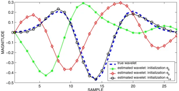
Fig. 1. Estimated wavelet for different initializations.
To estimate the respective orders and of the AR and MA parts, in [8], [36], we have proposed to use a Kurtosis maxi-mization criterion. Although this criterion is efficient in many cases, it may not be very satisfactory in certain situations. Al-ternatively, we propose to estimate and by use of an exhaus-tive search. For this aim, we use a nested loop with and as indices. The optimum for is obtained when the criterion is minimum. We will call SEM P (P for Prony) the parameter estimation procedure that we have just proposed that consists in applying the SEM algorithm followed by an ARMA extension of the initial MA wavelet estimate.
IV. INITIALMA MODELORDERSELECTION ANDMAXIMUM POSITIONSELECTION
We now consider two important practical issues for the SEM P algorithm working properly. Note that these consider-ations can be useful for many other algorithms.
A. Initial MA Model Order Selection
In this section, we explain how the length of the initial MA wavelet can be selected. Our approach is based on an MSE criterion. The idea is to look for the order , for which the estimated wavelet is as close as possible to the true wavelet . Unfortunately, the true wavelet itself is not known in practice. As the wavelet length is in some (possibly large) interval , we consider all the wavelet estimates supplied by the SEM algorithm for these choices of . The MSE criterion would
lead to choosing . Since is
unknown, we estimated it as
(16)
If we compare the functions MSE: and
MSE: , we have checked on simulations that
they roughly behave in the same way (see Section V). Thus, a good choice for is
(17)
B. Maximum Position Selection
It is well known that the nonminimum phase structure of the wavelet makes its estimation complicated. One may think that, due to the stochastic approximation of the expectation in the first step of the SEM algorithm, it should not be sensitive to the initialization parameters, but this is not the case. This problem has already been pointed out in [37], where a simu-lated annealing version of the SAEM algorithm is proposed to solve the deconvolution problem.
As mentioned previously, the wavelet estimation is not ro-bust with respect to the initialization. If we initialize with the vector , , that has all entries equal to zero ex-cept the th one which is equal to 1, we observe that the SEM algorithm yields an estimate of with its maximum at entry . As an example, Fig. 1 shows an estimated wavelet obtained for distinct initializations in the case of Ricker’s wavelet.
To understand this phenomenon, let us remark that the knowl-edge of the data vector , given by , permits us to recover up to a time translation and an amplitude shift but not , since we also have
(18) for any amplitude and any delay , where and de-note, respectively, the function delayed by and delayed by . This explains why the SEM algorithm does not look for a wavelet with its maximum, apart from the position of the nonzero component of the initial guess . This interpretation is impressively confirmed by simulations: For more than 99% of the simulations, the estimated wavelet has its maximum at po-sition when it is initialized with .
Fig. 2. Gaussian mixture reflectivity sequence.
To end this discussion, let us remark that one should not con-clude from relation (18) that any initialization would be satis-factory due to the delay compensation between and . In-deed, this would be true only if the searched wavelet support were infinite. Here, bad initialization may cause poor estimation of the wavelet, due to the limited wavelet support. We have seen in Section II that limiting the support is necessary to achieve a good parameter estimation performance.
We propose a deterministic procedure for initializing the MA wavelet estimate. First, we have performed the decon-volution for each initialization of . Then, we note if the estimator obtained from initialization has a positive derivative at the origin, and if it is negative. It can be checked on simulations that
changes sign for entries corresponding to local optima of the true wavelet. A justification of this phenomenon is presented in the Appendix. Simulations on several examples show the very good practical behavior of this technique (see Section V). The retained solution for the maximum position is chosen among the entries of for which its sign changes, by selecting the one for which the kurtosis of the estimated reflectivity is maximum.
V. RESULTS
In this section, we evaluate performance of the proposed methods for the wavelet estimation and for the SEM algorithm initialization, through simulations and real data experiments.
A. Simulation Results
We will define the SNR as
SNR (19)
where is the source wavelet energy and is the wavelet
length: .
1) Reflectivity and Noise Parameters: The reflectivity
se-quence samples are distributed according to a Gaussian mixture
Fig. 3. Noisy seismic data (SNR= 10 dB).
Fig. 4. MSE: “—” ; MSE: “- - -”.
TABLE I
SEM DECONVOLUTION: ESTIMATEDPARAMETERS FORSNR= 13 dB
with , , , and .
A typical reflectivity sequence is presented in Fig. 2. The cor-responding seismic trace is presented in Fig. 3. This synthetic trace is generated by using the long convolution wavelet shown in Fig. 5.
To show that it is better to use a truncated wavelet estimator instead of a full length one, we compare the quality of the es-timators for parameters in both cases. In addi-tion, we check this for SNR 8 dB and SNR 13 dB, which roughly corresponds to the range of SNR values in practical ex-periments. Results are presented in Tables I and II. It clearly appears that better parameter estimation for is achieved with the truncated wavelet. One main difference
be-TABLE II
SEM DECONVOLUTION: ESTIMATEDPARAMETERS FORSNR= 8 dB
TABLE III
KURTOSIS OF^rFOR THESEM PROCEDUREINITIALIZEDFROM THEFIRST
LOCALMAXIMA OF^h DETECTEDFROMC (WAVELET OFFIG. 5)
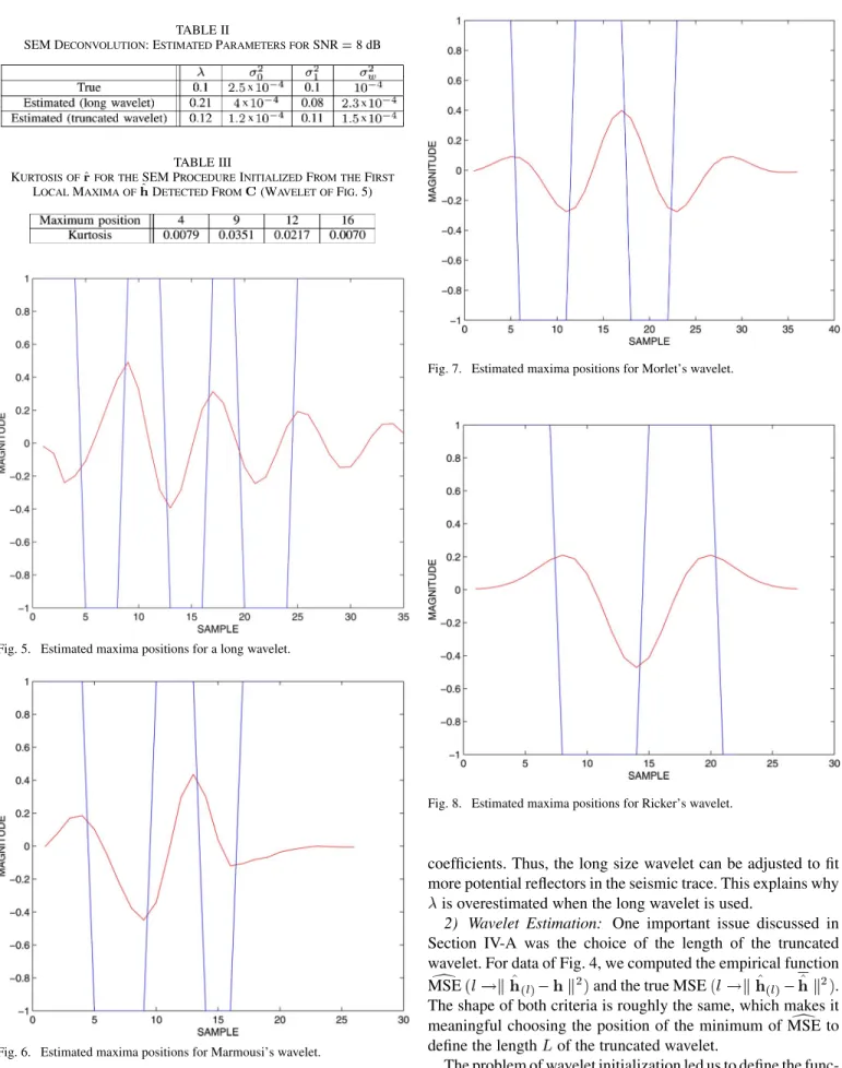
Fig. 5. Estimated maxima positions for a long wavelet.
Fig. 6. Estimated maxima positions for Marmousi’s wavelet.
tween using truncated and full size wavelet is that in the second case there are more degrees of freedom; in particular, the trun-cated wavelet can be seen as a full size one with zeroed last
Fig. 7. Estimated maxima positions for Morlet’s wavelet.
Fig. 8. Estimated maxima positions for Ricker’s wavelet.
coefficients. Thus, the long size wavelet can be adjusted to fit more potential reflectors in the seismic trace. This explains why
is overestimated when the long wavelet is used.
2) Wavelet Estimation: One important issue discussed in
Section IV-A was the choice of the length of the truncated wavelet. For data of Fig. 4, we computed the empirical function
MSE and the true MSE .
The shape of both criteria is roughly the same, which makes it meaningful choosing the position of the minimum of MSE to define the length of the truncated wavelet.
The problem of wavelet initialization led us to define the func-tion (see Section IV-B). As mentioned in Section IV-B, initial-izations with wavelets with only one nonzero entry at a transi-tion of functransi-tion are retained. The kurtosis of the deconvolved sequence with the corresponding estimated wavelets can be seen
Fig. 9. Estimated long wavelet by a standard SEM procedure.
Fig. 10. Estimated Marmousi’s wavelet.
in Table III. The maximum of the kurtosis is achieved for ini-tialization at position 9 which corresponds to the wavelet maximum position.
We tested the standard SEM procedure [4] with several wavelets. They are represented in Figs. 5–8 together with the corresponding functions. Vertical lines represent the tran-sitions of between values and . We check that in all cases there is a good match between these transitions and the local optima of the wavelet. Figs. 5–8 show the corresponding deconvolution wavelets. We can see that the short wavelets (Figs. 10–12) are well estimated, which justifies using the
Fig. 11. Estimated Morlet’s wavelet.
Fig. 12. Estimated Ricker’s wavelet.
standard SEM procedure in such cases. On the contrary, the last part of the long wavelet is poorly estimated.
Now, let us show that the proposed SEM P wavelet estima-tion procedure works better for long wavelets than the standard SEM. Indeed, we can observe in Fig. 13 that the two-step esti-mation (truncated wavelet estiesti-mation followed by Prony exten-sion) achieves almost perfect long wavelet recovery. Figs. 9 and 13 show the significant gain of the SEM P against the SEM. Furthermore, to study improvements brought by the deconvolu-tion method, we consider the following performance indices:
and (20)
represents the error energy of the estimated wavelet, while represents the error of noiseless data
reconstruc-Fig. 13. Estimated wavelet by SEM+ P.
TABLE IV
MSE ANDMSE PERFORMANCEINDICES FORSEMANDSEM+ P METHODS(WAVELET OFFIG. 5)
tion, that is, the convolution of wavelet and reflectivity. Indeed, direct comparison of and is not suitable since is a sparse spike train sequence and thus very small reflector location off-sets may lead to high MSE .
Table IV confirms the improvement of the performance in-dices and [see (20)], with the SEM P pro-cedure compared to the standard SEM when applied to a long wavelet.
3) Reflectivity Estimation: Once the wavelet and model distribution parameters are estimated, we are able to recover the reflectivity sequence by means of the MPM algorithm. We are going to see that the quality of the estimator of strongly influences the estimation performance of .
The reflectivity sequence estimated by the SEM MPM and the (SEM P) MPM algorithms are given, respectively, in Figs. 14 and 15. Note that after applying the algorithms, it may occur that instead of one reflector two neighboring reflectors are found, either contiguous or separated by only one sample. Then, a postprocessing procedure can be applied to fuse these reflectors at their gravity center with cumulated amplitudes [4]. With the SEM MPM approach (Fig. 14), there are often many neighboring strong reflectors, which prevents applying this technique, while it has been possible to apply it with the (SEM P) MPM (Fig. 15) because distinct reflectors had sufficiently separated contributions, leading to much better results than the standard SEM MPM procedure (Fig. 14).
Fig. 14. Estimated reflectivity sequence by SEM+ MPM (SNR = 8 dB).
Fig. 15. Estimated reflectivity sequence by (SEM+ P) + MPM (SNR = 8 dB).
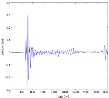
Fig. 16. Data record (trace 602).
B. Real-Data Experiments
Here, we consider real data acquired by IFREMER,1
con-sisting of seismic traces obtained from an innovative manner for synchronizing a cluster of air guns to achieve deeper penetra-tion. The fact that the sources are not synchronized in their firing
1French Research Institute for Exploitation of the Sea—Institut Français de
TABLE V
ESTIMATEDPARAMETERS FORSHOT1AND40,ANDMEAN OF50 SHOTS
Fig. 17. Full length estimated wavelet.
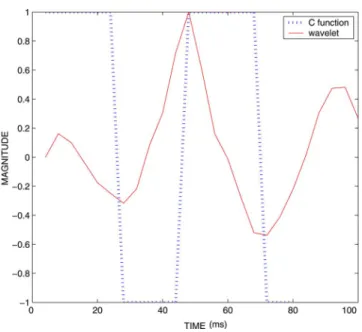
Fig. 18. Truncated estimated wavelet andC function.
order but on their time of maximum energy will decrease the signal bandwidth, and increase significantly the low-frequency content, and thus, the penetration. Each source is composed of 13 air guns, shooting a wavelet every 20 s with spectrum band-width 0–128 Hz. The multitrace streamer is composed of 360 clusters of 16 hydrophones. Its role is to improve the SNR by summing the received signals. The length of the streamer is 4.5 km and each cluster is separated by 12.5 m.
Fig. 19. MSE.
Fig. 20. Estimated wavelet by SEM+ P.
A typical recorded trace is presented in Fig. 16. Fig. 17 shows the full length wavelet estimated by SEM, while Fig. 18 repre-sents a truncated wavelet estimated by SEM together with the corresponding function. The wavelet in Fig. 17 does not cor-respond to the kind of wavelet generated by air guns.
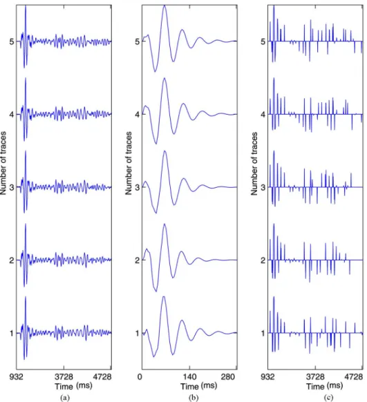
Fig. 19 shows that a good choice for the truncated wavelet length is 130 ms and Fig. 20 shows the Prony extension of the truncated wavelet estimate (SEM P estimate). Fig. 21 shows the deconvolution results obtained for several traces. Fig. 22 presents the wavelets estimated by the SEM P algorithm for different recorded seismic traces. We can observe that these wavelets are somewhat distinct, and thus, wavelet estimation
Fig. 21. (a) Real data (traces 402 to 406). (b) Estimated wavelet by SEM+ P. (c) Estimated reflectivity by (SEM + P) + MPM.
is necessary on each trace for proper recovery of reflectivity. However, there is a good similarity among them, and thus, the wavelet estimated for one trace could be a good initialization candidate for the deconvolution of the other traces.
The parameters estimated with the SEM al-gorithm are presented in Table V. The noise variance seems to be the parameter that more varies among traces.
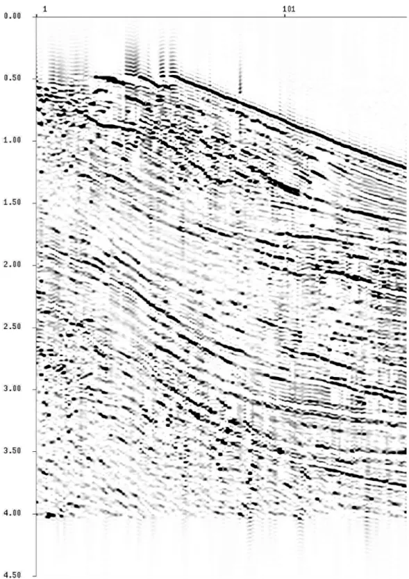
The seismic profile is presented in Figs. 23 and 24. We can see the deconvolution results obtained with our approach. On raw data presented in Fig. 23, the main reflectors are about 200-ms width (see seafloor, for example), and composed of an alterna-tion of two black and three white phases. In Fig. 24, after de-convolution, the reflectors are reduced to a single black phase, about 70 ms wide. Thus, the deconvolution, as expected, im-proves substantially the resolution of the section. The decrease of the signal width enables us to define more precisely the re-lationships between the different seismic units: For example, it is now much easier to follow the top of the erosional surface at the top left of the seismic line. It helps discriminating real events from artifacts: A seismic reflector, about 300 ms below the seafloor, with a negative polarity, the polarity and existence of which were not obvious, is now well imaged. Weaker
Fig. 23. Seismic profile. Y-label: shot number. X-label: time (s).
bouncing of the major reflectors are now apparent (see, for ex-ample, reflectors just below the seafloor).
VI. CONCLUSION
In this paper, we have proposed a new approach for blind de-convolution of seismic data in the presence of a long wavelet.
We have shown that the estimation of a truncated wavelet fol-lowed by an ARMA extension (SEM P) yields improved wavelet estimation, compared to the classical SEM approach. We have also proposed a new method for choosing the truncated wavelet order. Furthermore, an efficient procedure has been pro-posed for the wavelet initialization in the SEM algorithm.
Simu-Fig. 24. Deconvolved seismic profile. Y-label: shot number. X-label: time (s).
lations and real-data experiments have shown that our approach achieves significant improvement.
APPENDIX
In this section, we justify why the proposed criterion for max-imum position selection works efficiently, as shown in the simu-lation part. Let us recall, as discussed in Section IV-B, that when
the impulse response is initialized with one at the th entry and zeros at other entries, the SEM algorithm converges to a solution where the estimated has its maximum at position . In other words, we can say that the SEM algorithm looks for a solution that minimizes the norm error with a max-imum constraint at position .
Let us rephrase this idea in the continuous time domain. We are led to search for a solution that achieves minimum error
norm under the null derivative constraint . In mathe-matical terms, we are considering the following constrained op-timization problem:
(21) Equivalently, problem (21) can be rewritten in the Fourier trans-form domain
(22) where denotes the Fourier transform of and is the signal bandwidth. Using Lagrange multipliers (see, for instance, [38]) and introducing real and complex variations of yields the following conditions upon the solution of problem (22), denoted
by :
(23) Indeed, considering the functional
(24) and denoting by any real valued small variation of , the optimality constraint
yields
(25) leading thus to the first equation of (23). The second equation of (23) is derived in a similar way by considering imaginary small variation of . Then, summing both equations of (23) yields (26) with . Then, the solution of (22) is of the form (27)
Now, let us denote , which
cor-responds to the true wavelet in the noise-free case. After we insert solution (27) in the constraint equation
, it follows:
(28) Thus, from (27) and (28), we get the time-domain solution
(29)
Now, let us remark that
(30)
Clearly, if , changes sign at if has a
local optimum at point . This shows that, providing the true wavelet has an horizontal tangent at point 0, the derivative of the estimated wavelet changes sign around point [note that the term in the parenthesis in (30) is always positive]. We have checked that this result remains true for wavelets with small tangent slopes at point 0 which corresponds to most practical situations, where wavelets have a smooth shape and thus small slope at the origin.
ACKNOWLEDGMENT
The authors would like to thank B. Marsset and T. Yannick for their data.
REFERENCES
[1] E. A. Robinson and S. Treitel, Geophysical Signal Analysis. Engle-wood Cliffs, NJ: Prentice-Hall, 1980, pp. 152–161.
[2] O. Rosec and J. M. Boucher, “Bayesian estimation of non-minimum phase wavelets applied to marine reflection seismic data,” in Proc. Int. Conf. Acoust. Speech Signal Process., 1999, vol. 5, pp. 2797–2800. [3] J. M. Mendel, Optimal Seismic Deconvolution: An Estimation-Based
Approach. New York: Academic, 1983.
[4] O. Rosec, J. M. Boucher, B. Nsiri, and T. Chonavel, “Blind marine seismic deconvolution using statistical MCMC methods,” IEEE J. Ocean. Eng., vol. 28, no. 3, pp. 502–512, Jul. 2003.
[5] J. M. Mendel, “Tutorial on higher-order statistics (spectra) in signal processing and system theory: Theoretical results and some applica-tions,” Proc. IEEE, vol. 79, no. 3, pp. 278–305, Mar. 1991.
[6] D. L. Donoho, “On minimum entropy deconvolution,” in Applied Time Series Analysis, D. Findley, Ed. New York: Academic, 1981, pp. 556–608.
[7] M. Boumahdi, “Blind identification using the Kurtosis with applica-tions to field data,” Signal Process., vol. 48, no. 3, pp. 205–216, 1996. [8] M. Boujida and J. M. Boucher, “Higher order statistics applied to wavelet identification of marine seismic signal,” in Proc. 8th Eur. Signal Process. Conf., 1996, vol. 1, pp. 137–141.
[9] C. L. Nikias, “ARMA bispectrum approach to nonminimum phase system identification,” IEEE Trans. Acoust. Speech Signal Process., vol. 36, no. 4, pp. 513–524, Apr. 1988.
[10] A. Larue, J. I. Mars, and C. Jutten, “Frequency-domain blind deconvo-lution based on mutual information rate,” IEEE Trans. Signal Process., vol. 54, no. 5, pp. 1771–1781, May 2006.
[11] J. M. Mendel, Maximum-Likelihood Deconvolution. New York: Springer-Verlag, 1990, pp. 7–59.
[12] K. F. Kaaresen, “Deconvolution of sparse spike trains by iterated window maximization,” IEEE Trans. Signal Process., vol. 45, no. 5, pp. 1173–1183, May 1997.
[13] C. P. Robert, The Bayesian Choice. New York: Springer-Verlag, 1994, pp. 344–355.
[14] A. P. Dempster, N. M. Laird, and D. B. Rubin, “Maximum likelihood from incomplete data via the EM algorithm,” J. Roy. Statist. Soc. Ser. B, no. 39, pp. 1–38, 1977.
[15] M. Feder and E. Weinstein, “Parameter estimation of superimposed signals using the EM algorithm,” IEEE Trans. Acoust. Speech Signal Process., vol. ASSP-36, no. 4, pp. 477–489, Apr. 1988.
[16] G. Celeux, D. Chauveau, and J. Diebolt, “Stochastic versions of the EM algorithm,” J. Stat. Comput. Simul., vol. 55, pp. 287–314, 1996. [17] G. Celeux and J. Diebolt, “The SEM algorithm: A probabilistic teacher
algorithm derived from the EM algorithm for the mixture problem,” Comput. Stat., vol. 2, pp. 73–82, 1985.
[18] G. Celeux and J. Diebolt, “A stochastic approximation type EM algorithm for the mixture problem,” Stoch. Stoch. Rep., vol. 22, pp. 747–761, 1989.
[19] M. Lavielle, “Bayesian deconvolution of Bernoulli-Gaussian pro-cesses,” Signal Process., vol. 33, pp. 67–79, 1993.
[20] A. Doucet and P. Duvaut, “Bayesian estimation of state-space models applied to deconvolution of Bernoulli-Gaussian processes,” Signal Process., vol. 57, pp. 147–161, 1997.
[21] J. Idier and Y. Goussard, “Multichannel seismic deconvolution,” IEEE Trans. Geosci. Remote Sens., vol. 31, no. 5, pp. 961–980, Sep. 1993. [22] Q. Cheng, R. Chen, and T. Li, “Simultaneous wavelet estimation and
deconvolution of reflection seismic signals,” IEEE Trans. Geosci. Re-mote Sens., vol. 34, no. 2, pp. 377–384, Mar. 1996.
[23] J. Marroquin, S. Mitter, and T. Poggio, “Probabilistic solution of ill-posed problems in computational vision,” J. Amer. Stat. Assoc., vol. 82, pp. 76–89, 1987.
[24] B. Chalmond, “An iterative Gibbsian technique for reconstruction of m-ary images,” Pattern Recognit., vol. 22, pp. 747–761, Jun. 1989. [25] S. Geman and D. Geman, “Statistic relaxation, Gibbs distribution and
the Bayesian restoration of images,” IEEE Trans. Pattern Anal. Mach. Intell., vol. PAMI-6, no. 6, pp. 721–741, Nov. 1984.
[26] J. Besag, “On the statistical analysis of dirty pictures,” J. Roy. Stat. Soc., vol. 48, pp. 259–302, 1986.
[27] B. Nsiri, J. M. Boucher, and T. Chonavel, “Multichannel blind decon-volution. Application to marine seismic,” in Proc. OCEANS, Sep. 2003, vol. 5, pp. 22–25.
[28] P. Farcy, “System acquisition of submarine seismic,” IFREMER, Bre-tagne, France, ESSR4 Campaign Rep., DNIS/ESI/ENS/DTI/99-007, 1999.
[29] T. Chonavel, Statistical Signal Processing, Modelling and Estima-tion. New York: Springer-Verlag, 2002, pp. 166–182.
[30] T. W. Parks and C. S. Burrus, Digital Filter Design. New York: Wiley, 1987, pp. 226–228.
[31] W. Gilks, S. Richardson, and D. Spiegelhalter, Markov Chain Monte Carlo in Practice. London, U.K.: Chapman & Hall, 1996, pp. 1–17. [32] A. E. Gelfand and A. F. M. Smith, “Sampling-based approaches to calculating marginal densities,” J. Roy. Stat. Soc., vol. 85, no. 410, pp. 398–409, 1990.
[33] O. Rosec, “Déconvolution Aveugle Multicapteur en Sismique Réflexion Marine Trés haute Résolution,” Ph.D. dissertation, Univ. Bretagne Occidentale, Brest, France, 2000.
[34] O. Rabaste and T. Chonavel, “Estimation of multipath channels with long impulse response at low SNR via an MCMC method,” IEEE Trans. Acoust. Speech Signal Process., vol. 55, no. 4, pp. 1312–1325, Apr. 2007.
[35] B. Nsiri, T. Chonavel, and J. M. Boucher, “SEM blind identification of ARMA models application to seismic data,” in Proc. Eur. Signal Process. Conf. (EUSIPCO), 2004, pp. 1099–1102.
[36] B. Nsiri, T. Chonavel, and J. M. Boucher, “Blind seismic deconvolution with long wavelet impulse response,” in Phys. Signal Image Process., Jan. 2003, pp. 5–8.
[37] M. Lavielle and E. Moulines, “A simulated annealing version of the EM algorithm for non-Gaussian deconvolution,” Stat. Comput., vol. 7, pp. 229–236, 1997.
[38] J. L. Troutman, Variational Calculus and Optimal Control: Optimiza-tion With Elementary Convexity. New York: Springer-Verlag, 1996, pp. 97–186.
Benayad Nsiri (S’02–A’04) was born in Temara,
Morocco, in 1974. He received the D.E.A. degree (French equivalent of M.Sc. degree) in electronics from the Occidental Bretagne University, Brest, France, in 2000 and the Ph.D. and the M.B.I. degrees in computer sciences from Ecole Nationale Supérieure des Télécommunications (ENST) de Bre-tagne, Brest, France, in 2004 and 2005, respectively. Currently, he is an Assistant Professor at the Faculty of Sciences Ain Chock, Hassan II Univer-sity, Casablanca, Morocco, a Member Associate in GSCM-LRIT group, Rabat Morocco, and a Member Associate at the Signal and Communication Department, ENST. His research interests include but are not restricted to signal processing, adaptive techniques, blind deconvolution, MCMC methods, seismic data, and higher order statistics.
Thierry Chonavel received the Ph.D. degree in
signal processing from Ecole Nationale Supérieure des Télécommunications (ENST), Paris, France, in 1992. His thesis was about trigonometric moment problems and array processing.
He joined the Groupe des Ecoles des Telecom-munications (GET) in 1993. Currently, he is a Professor at Ecole Nationale Supérieure des Télé-communications (ENST) de Bretagne, Brest, France. His research interests are in signal processing and communications with works in adaptive processing, code division multiple access (CDMA), geolocalization, automotive radars, and applications related to underwater acoustics (ocean tomography and seismic).
Jean-Marc Boucher (M’84–SM’05) received the
Engineering degree in telecommunications from the Ecole Nationale Supérieure des Telecommunications (ENST), Paris, France, in 1975 and the Habilitation à Diriger des Recherches degree from the University of Rennes 1, Rennes, France, in 1995.
Currently, he is a Professor at the Department of Signal and Communications, ENST, where he is also Education Deputy Director. He is the Deputy Manager of a National Scientific Research Center Laboratory, Traitement Algorithmique et Matériel de la Communication, de l’Information et de la Connaissance (TAMCIC), UMR 2872, Brest, France. His current research interests are related to statistical signal analysis including estimation theory, Markov models, blind deconvo-lution, wavelets, and multiscale image analysis. These methods are applied to radar and sonar images, seismic signals, and electrocardiographics. He has published about 100 technical articles in these areas in international journals and conferences.
Hervé Nouzé received the Engineering degree from
Ecole Nationale Supérieure des Mines de Nancy in 1992, and the degree from Ecole Nationale du Pétrole et des Moteurs in 1993.
Since 1995, he has been a Geophysicist at the Marine Geosciences Department, Institut Français de Recherche pour L’Exploitation de la Mer (IFREMER), Bretagne, France. His main research interest is the development of geophysical (mainly seismic) methods to detect and quantify the occur-rence of gas and gas hydrates in marine sediments.