HAL Id: hal-02441978
https://hal-cea.archives-ouvertes.fr/hal-02441978
Submitted on 16 Jan 2020
HAL is a multi-disciplinary open access
archive for the deposit and dissemination of sci-entific research documents, whether they are pub-lished or not. The documents may come from teaching and research institutions in France or abroad, or from public or private research centers.
L’archive ouverte pluridisciplinaire HAL, est destinée au dépôt et à la diffusion de documents scientifiques de niveau recherche, publiés ou non, émanant des établissements d’enseignement et de recherche français ou étrangers, des laboratoires publics ou privés.
nuclear reactor thermalhydraulics
D. Bestion, A. de Crecy, F. Moretti, R. Camy, A. Barthet, S. Bellet, J. Munoz
Cobo, A. Badillo, B. Niceno, P. Hedberg, et al.
To cite this version:
D. Bestion, A. de Crecy, F. Moretti, R. Camy, A. Barthet, et al.. Review of uncertainty methods for CFD application to nuclear reactor thermalhydraulics. NUTHOS 11- The 11th International Topical Meeting on Nuclear Reactor Thermal Hydraulics, Operation and Safety, Oct 2016, Gyeongju, South Korea. �hal-02441978�
1
Review of Uncertainty methods for CFD application to nuclear reactor
thermalhydraulics
Bestion D , de Crecy A
CEA-Grenoble, 17 rue des martyrs, 38054 GRENOBLE FRANCE [email protected]
Moretti F
NINE – Nuclear and Industrial Engineering [email protected]
Camy R
EDF-R&D, 8 quai Watier BP 49, 78401 Chatou, FRANCE [email protected]
Barthet A, Bellet S
EDF – SEPTEN, 12-14 avenue Dutriévoz, 69628 Villeurbanne , FRANCE [email protected], [email protected]
Munoz Cobo J L
Dpto. Ingenieria Nuclear, Universidad Politecnica de Valencia, Camino de Vera 14, 46022 VALENCIA, SPAIN
Badillo A, Niceno B
Paul Sherrer Institute, 5232 Villigen Switzerland [email protected], [email protected]
Hedberg P
Swedish Radiation Safety Authority, Dept. of Nuclear Power Plant Safety SE-171 16 Stockholm, Solna strandväg 96, SWEDEN
Scheuerer M
Gesellschaft für Anlagen- und Reaktorsicherheit 85748 Garching b. Munchen, GERMANY [email protected]
Nickolaeva A
OKB Gidropress, Russia
ABSTRACT
In the past ten years, the Working Group for the Analysis and Management of accidents (WGAMA) initiated activities to promote the use of CFD for Nuclear Reactor Safety (NRS). Best Practice Guidelines were written which are applicable to single phase CFD. Assessment requirements were also addressed. These activities provided more confidence in the application of CFD for safety by defining some conditions and requirements. However, no applicative methods were written about a possible quantitative evaluation of the uncertainty of predictions which is mandatory for complementing a Best-Estimate approach within a nuclear reactor licensing framework. A new activity reported here was then initiated to review the methodologies for determination of the uncertainty of CFD predictions applied to reactor thermalhydraulics. An OECD report [1] was written which is summarized in this paper. A proposal for CFD UQ global approach shows the link between PIRT, Verification, Validation,
2
and Uncertainty Quantification (UQ). The various sources of uncertainty are identified. Methods for uncertainty quantification are then reviewed, considering accuracy extrapolation and uncertainty propagation methods (with the possible use of meta-models). Then a few methods or elements of methods are summarized. The role of Separate Effect Tests and Integral Effect Tests in the UQ process is mentioned. Finally some conclusions are drawn, remaining needs are identified, and recommendations for further R&D and benchmarking of methods are given to progress on this topic.
KEYWORDS
Computational Fluid Dynamics, Uncertainty Quantification
1. INTRODUCTION
Single phase CFD is more and more used for design and safety issues related to Light Water Reactor (LWR) thermalhydraulics. In the past ten years, the Working Group for the Analysis and Management of Accidents (WGAMA) initiated activities to promote the use of CFD for Nuclear Reactor Safety (NRS). A list of safety issues for which CFD may bring a real benefit was established. Best Practice Guidelines were written which are applicable to single phase CFD. Assessment requirements were also addressed in a report with some particular attention to a few safety issues. These activities provided more confidence in the application of CFD for safety by defining the conditions and requirements for obtaining reliable predictions. However, no applicative methods were written about a possible quantitative evaluation of the uncertainty of predictions, which is mandatory in a Best-Estimate approach. A new activity was then initiated to review the methodologies for determination of the uncertainty of CFD predictions applied to reactor thermalhydraulics. An OECD report [1] was written which is summarized in this paper. This is a very recent domain of investigation and the reported activity is rather limited. Only some prospective works are in progress in different communities. However one may first list what exists and conclude on the remaining needs. A comparison with system codes may be useful since available methods are rather mature as the BEMUSE project has shown.
The OECD CFD Best Practice Guidelines (BPG) report [2] gives some concepts to reach good quality for CFD results in a thermalhydraulics Safety context. Based on these concepts, which underline the key role of the physical analysis, one can introduce first, in this document, a more detailed proposal for CFD UQ global approach in showing the link between PIRT/Verification/Validation/Uncertainty Quantification. The domain of possible application of single-phase CFD for NRS is first recalled. Then the various sources of uncertainty are identified. Methods for uncertainty quantification are then reviewed, considering accuracy extrapolation and uncertainty propagation methods (with the possible use of meta-models). Then a few methods or elements of methods are summarized in respective subsections. The role of Separate Effect Tests and Integral Effect Tests in the UQ process is mentioned. Finally some conclusions are drawn, remaining needs are identified, and recommendations for further R&D and benchmarking of methods are given to progress on this topic.
3
Within the past activity of WGAMA on CFD application to NRS the WG2 (writing Group 2) produced a report (Smith at al, 2015, [3]) with a critical review of the NRS problems where the use of CFD is needed for the analysis or where its use is expected to result in major benefits. The focus was on the use of CFD techniques for single-phase problems relating to NRS. Considering only single phase issues it appears that most of them are related to turbulent mixing problems, including temperature mixing or mixing of chemical components in a multi-component mixture (boron in water, hydrogen in air,…):
• Erosion, corrosion and deposition • Boron dilution
• Mixing: stratification/hot-leg heterogeneities
• Heterogeneous flow distribution (e.g. in SG inlet plenum causing vibrations, etc.) • BWR/ABWR lower plenum flow
• PTS (pressurised thermal shock) • Induced break
• Thermal fatigue • Hydrogen distribution
• Chemical reactions/combustion/detonation
• Special considerations for advanced (including Gas-Cooled) reactors
In some of these mixing issues, density differences induce buoyancy effects which have a significant influence on the mixing: cold water may be mixed with hot water, borated water mixed with non-borated water, hydrogen with air, etc.
Among the mixing problems listed here above, some are steady-state or quasi-steady-state flows (hot-leg heterogeneities, heterogeneous flow distribution, lower plenum flow, Induced break, mixing between core sub-channels,…) and some other are rather slow and long transients (boron dilution, PTS, hydrogen distribution, etc.). Only a few consider phenomena at a small time scale (combustion, thermal fatigue).
In summary, the development and assessment of methods for uncertainty evaluation of CFD should focus first on mixing problems with density effects in steady state or in slow transients, since it would cover most envisaged applications.
3 THE LINK BETWEEN PIRT, SCALING, VERIFICATION, VALIDATION AND UNCERTAINTY QUANTIFICATION
The reactor safety demonstration requires the analysis of complex problems related to accident scenarios. The experiments cannot reproduce at a reasonable cost the physical situation without any simplification or distortion and the numerical tools cannot simulate the problem by solving the exact equations. Only reduced scale experiments are feasible to investigate the phenomena and only approximate system of equations may be solved to predict time and/or space averaged parameters with errors due to imperfections of the closure laws and to numerical errors. Therefore complex methodologies are necessary to solve a problem including a PIRT analysis, a scaling analysis, the selection of scaled Integral Effect Tests (IET) or Combined effect tests (CET) and Separate Effect Tests, the selection of a numerical simulation tool, the Verification and Validation of the tool, the code application to the safety issue of interest and the use of an uncertainty method to determine the uncertainty of code prediction. This global approach is illustrated in Figure 1.
4
Figure1. Methodology for Solving a complex Reactor Thermalhydraulic Issue
3.1 The PIRT
Phenomena identification is the process of analyzing and subdividing a complex system thermal-hydraulic scenario (depending upon a large number of thermal-hydraulic quantities) into several simpler processes or phenomena. One can discern the dominant parameters (Figures of Merit - FoM) with the parameters which have an influence on FoM. FoMs play a key role directly on the safety criterion. Depending on the safety issue, the FoM can be a scalar or a multidimensional field value (over space and/or time) or a maximum value. The FoM can be made non-dimensional. The required accuracy on the FoM has to be given. Ranking means here the process of establishing a hierarchy between identified phenomena with regards to their influence on the FoMs.
PIRT is a formal method described in Wilson & Boyack (1998, [4]). Its use is recommended by OCDE WGAMA BPG [2]. The main steps of the physical analysis are:
• Establish the purpose of the analysis and specify the reactor transient (or situation) of interest
• Define the dominant parameters or FoM (figures of Merit)
• List the involved physical phenomena and associated parameters. Identify and rank key phenomena (or the parameters associated to each phenomenon for a more accurate PIRT) with respect to their influence on the FoM.
• Identify dimensionless numbers controlling the dominant phenomena
PIRT can be based on expert assessment, on analysis of some experiments, and on sensitivity studies using simulation tools. One can start with expert assessment and then iterate with some sensitivity studies to refine the PIRT conclusions.
3.2 Scaling
Scaling of an experiment is the process of demonstrating how and to what extent the simulation of a physical process (e.g. a reactor transient) by an experiment at a reduced scale (or at
5
different values of some flow parameters such as pressure and fluid properties) can be sufficiently representative of the real process in a reactor.
Scaling applied to a numerical simulation tool is the process of demonstrating how and to what extent the numerical simulation tool validated on one or several reduced scale experiments (or at different values of some flow parameters such as pressure and fluid properties) can be applied with sufficient confidence to the real process.
Scaling leads to predict a result for the reactor from a scaled experiment, as mentioned in Oberkampf & Roy [5].
When solving a reactor thermalhydraulic issue the answer to the issue may be purely experimental; the experiments can tell what would occur in the reactor with sufficient accuracy and reliability (red arrow in Figure 1). But most often both experiments and simulation tools are used to solve the issue and the simulation tool is used to extrapolate from experiments to reactor situation - this is the upscaling process- and the degree of confidence on this extrapolation is part of the scaling issue.
The extrapolation to a reactor situation made by a single phase CFD tool induces several aspects and raises several questions:
• How to guarantee that a CFD code can extrapolate from reduced scale validation experiment to full scale application?
• How to extrapolate the nodalization from reduced scale validation experiment to full scale application?
• How to extrapolate:
o from one fluid to another fluid?
o to a different value of the Re number and/or to a different value of any other non-dimensional numbers?
In any case the numerical simulation of the scaled experiments has a given accuracy defined by the error on some target parameters and one should determine how the code error changes when extrapolating to the reactor situation.
Therefore scaling associated to CFD application is part of the CFD code uncertainty evaluation and is a necessary preliminary step in this uncertainty quantification.
Both scaling and uncertainty are closely related to the process of Validation and Verification. The definition of metrics for the validation is also part of the issue.
For application in nuclear reactor safety, a comprehensive methodology named H2TS (“Hierarchical Two Tiered Scaling”) was developed by a Technical Program Group of the U.S. NRC under the chairmanship of N. Zuber (1991) [6]. This work provided a theoretical framework and systematic procedures for carrying out scaling analyses. As the name suggests, the approach is based on using a progressive and hierarchized scaling organized in two basic steps. The first one goes from top to down, T-D, and the second step goes from bottom to up (B-U)
The T-D step is organized at the system or plant level and is used to deduce non-dimensional groups that are obtained from mass (M), energy (E) and momentum (MM) conservation equations, obtained from the systems that have been considered as important in a PIRT. These non-dimensional groups are used to establish the scaling hierarchy i.e. what phenomena have priority in order to be scaled, and to identify what phenomena must be included in the bottom-up analysis.
6
The second part of the H2TS methodology is the B-U analysis. This is a detailed analysis at the component level that is performed in order to assure that all relevant phenomena are properly represented in the balance equations that govern the evolution of the main magnitudes in the different control volumes.
The scaling analysis is based on the PIRT but it can also support the PIRT by helping in the ranking of phenomena. The PIRT may lead to the scaling of experimental data of IET type and may also identify the need of SETs, when using for example the H2TS method with both a top-down and a bottom-up approache. The selection of the numerical tool (here a CFD code or a coupling of CFD with other thermalhydraulic codes) must be consistent with the PIRT: the selected physical model should be able to describe the dominant phenomena. Then the selected numerical tool must be verified and fully validated in particular on the selected IETs and SETs. The example shown in Figure 1 corresponds to investigations of mixing problems in cold leg and Pressure Vessel of a PWR with ROCOM as IET and GEMIX as one of the SETs. Then the code application to the reactor transient must include an Uncertainty Quantification which may use code validation results to evaluate the impact of some sources of uncertainties.
3.3 Verification and Validation
V&V activities are dealing with numerical and physical assessment.
Verification is a process to assess the software correctness and numerical accuracy of the solution to a given physical model defined by a set of equations. The verification is performed to demonstrate that the implementation of the code numerical algorithms conforms to the design requirements, that the source code conforms to programming standards and language standards, and that its logic is consistent with the design specification. The verification is usually conducted by the code developers and, sometimes, independent verification is performed by the code users. Verification covers: equations implementation, calculation of convergence rate (for code and solution verification) [5]. Practically, verification consists in calculating some test cases with comparison to an analytical solution or a reference solution or in using the method of manufactured solutions.
Validation of a code is a process to access the accuracy of the physical models of the code based on comparisons between computational simulations and experimental data. The validation is performed to provide confidence in the ability of a code to predict the values of the safety parameters or parameters of interest. It may also quantify the accuracy. The results of a validation may be used to determine the uncertainty of some constitutive laws of the code. The validation can be conducted by the code developers and/or by the code users. The former case is called developmental assessment and the latter is called an independent assessment. A validation matrix is a set of selected experimental data for the purpose of extensive and systematic validation of a code. The validation matrix usually includes:
• basic tests
• separate effect tests or single effect tests (SETs)
• integral effect tests (IETs) or Combined effect tests (CETs) • nuclear power plant data
Various validation matrices can be established by code developers and/or code users for their own purposes.
Separate Effect Tests are experimental tests which intend to investigate a single physical process either in the absence of other processes or in conditions which allow measurements of the effects of the process of interest. SET may be used to validate a constitutive relation independently from the others.
7
Integral Effect Tests are experimental tests which intend to simulate the behavior of a complex system with all interactions between various flow and heat transfer processes occurring in various system components. IET relative to reactor accidental thermal-hydraulics can simulate the whole primary cooling circuit and simulate the accidental scenario through initial and boundary conditions.
For the two steps of validation the comparison of simulation results with measurements from experiments is a key point (starting with the metric definition). This comparison provides some elements used to determine the uncertainties from the models. The gap between calculations and experiment contributes to the uncertainty quantification but it can also set different parameters of the CFD code used (as turbulence model, numerical scheme,…). A method for synthesizing validation results in a table was proposed by A. Nikolaevna (See Appendix 2 in [1]);
3.4 Uncertainty quantification
Uncertainty Quantification (UQ) starts by clearly identifying the various sources of uncertainties. Sensitivity analysis can be used to identify among all sources of uncertainties the main contributors to the uncertainty of the Figures of Merit. Each source of uncertainty may be quantified. The validation may be used to quantify the model uncertainties and to measure the code accuracy. Then either extrapolation of accuracy or propagation of uncertainty methods can be used to determine the uncertainty of code predictions of a reactor issue.
Very often, in NRS context, the coupling or chaining of different codes dedicated to different branches of physics has to be considered when treating UQ of CFD results. The assembling of the different uncertainties could probably be included in a global design methodology for a safety demonstration.
4 THE VARIOUS SOURCES OF UNCERTAINTY IN CFD APPLICATIONS TO LWR Theoretically, the sources of uncertainty of single-phase CFD are the same as for system codes, but practically there are big differences in the relative weight of each source.
One may list the following sources of uncertainty of single-phase CFD application :
1 Initial and boundary conditions: the inlet flow parameters may be known with a rather high uncertainty when they result from a system code calculation which gives only 1D (area averaged) flow parameter whereas CFD needs 2D inlet profiles (potentially functions of time).
2 Uncertainties related to the physical models
a. Uncertainties related to the parameters of physical models: wall functions – if used – to express momentum and energy wall transfers and parameters of turbulence models (e.g. C1, C2, Cm, Prk and Pr ε of the k-ε model) are sources of uncertainties. Experts in turbulence may argue that these parameters were derived from basic flow configurations and should not be changed. However models may be used beyond their domain of applicability and one may assign uncertainties related to this extrapolation.
b. Uncertainties related to non-modelled physical processes and uncertainties related to the form of the models: models may have inherent limitations. For
example, any eddy viscosity model like k-ε or k-ω cannot predict a non-isotropic turbulence nor an inverse-cascade of energy from small turbulence scales to large ones.
8
c. Choice among different physical model options: when BPGs cannot give strong arguments to recommend one best model option, one may consider all the possible model options compatible with BPGs and consider the choice of the option as a source of uncertainty. This is a “categorical variable” in the extended propagation of uncertainty method described in section 6.
3 Uncertainties related to the numerical solution
a. Numerical uncertainties: they are related to the discretization and to the solving of the equations; they include time discretization errors, spatial discretization errors, iteration errors and round-off errors. BPG give recommendations to control these numerical errors. However, a certain level of residual error may be accepted if one can estimate the resulting uncertainty band on the prediction. b. Choice among different numerical options: when BPGs cannot give strong
arguments to recommend one best numerical option, one may consider all the possible numerical options compatible with BPGs and consider the choice of the option as a source of uncertainty. This is also a “categorical variable” in the extended propagation of uncertainty method described in section 6.
4 Simplification of the geometry: geometrical details of a reactor may have some impact on the resulting flow. In code applications, some simplifications of the geometry may be adopted and in all cases details smaller than the mesh size are not described. This induces some non-controlled errors which should be considered in the UQ process. 5 Uncertainties due to scaling distortions: there may be situations where one can
determine the uncertainty due to input parameters in a given range of flow conditions characterized by a geometry and the values of some non-dimensional numbers. In reactor applications it may occur that the geometry and values of some dimensional numbers are out of the given range. Then one should assign some extra uncertainty on final results due to the extrapolation to other geometry or other values to non-dimensional numbers.
6 Uncertainty due to measured previous data: Information coming from previous data may be used in a simulation such as the physical properties of fluid and solids. This information is known with some uncertainty which will also affect the global uncertainty of code predictions.
7 Uncertainty arising from physical instabilities/chaotic behavior: Non-linear dynamic systems (like Navier Stokes equations) can have under certain circumstances a chaotic behavior. Chaos results in long term unpredictability but determinism guarantees short term predictability. Chaotic behavior can be identified with small change in the input data. If the FoM exhibits a chaotic nature, it must be treated in a probabilistic framework.
5 CLASSIFICATION OF METHODS FOR UNCERTAINTY QUANTIFICATION Code uncertainty methodologies for reactor thermalhydraulics were first developed for system codes which simulate many kinds of transients in a very large range of single phase and two-phase conditions. They were based on either “propagation of the uncertainty of input parameters” (so called uncertainty propagation methods) or “accuracy extrapolation” methods (D’Auria & al. , 1995 [7]).
5.1 Methods based on propagation of uncertainties
The method using propagation of code input uncertainties for thermalhydraulics with a link to NRS issues follows the pioneering idea of CSAU [8], later extended by GRS (Glaeser et al.,
9
1994 [9]). It is the most often used class of methods. Uncertain input parameters are first listed including initial and boundary conditions, material properties, and closure laws. Probability density functions are determined for each input parameter. Then the parameters are sampled according to their probability functions and the reactor simulations are run with each set. In the GRS proposal a Monte Carlo sampling is performed with all input parameters being varied simultaneously according to their density function.
The Wilks theorem is often used to treat the results of uncertainty propagation. It makes it possible to estimate the boundaries of the uncertainty range on any code response with a given degree of confidence. The number of code runs is around 100 for an acceptable degree of confidence, even if slightly higher number of code runs, typically 150 to 200 is advisable to have a better accuracy on the uncertainty ranges of the code response.
More generally, propagation of uncertainties typically requires many calculations to reach convergence of statistical estimators which may be difficult with CFD because of large required CPU time. Fortunately, relatively simple statistical tools can give an estimate of the uncertainty resulting from datasets of limited size (bootstrap and Bayes formula for example).
In the domain of uncertainty propagation methods, there are three trends:
• The Monte-Carlo type method uses a rather large number of simulations with all uncertain input parameters being sampled according to their pdf. The resulting pdf of any code response is established and the accuracy does not depend on the number of uncertain input parameters.
• Use of meta-models: in an attempt to reduce the number of code simulations, some methods consider only the most influential uncertain input parameters and do a few calculations varying these input parameters in order to build a meta-model which will replace the code to determine the uncertainty on any code response with a low CPU cost: the Monte-Carlo method is used with these meta-models, with several thousands of runs. The use of meta-models (such as polynomial chaos expansion and kriging) became popular. These meta-models (or assimilated) provide a mapping between uncertain input parameters and Model results built on a limited number of Model evaluations. They necessarily rely on assumptions of regularity or continuity or shape of Model responses and should be considered with caution when these assumptions are difficult to verify. Basically in such a case, one might replace the non-convergence uncertainty of propagation methods that is rather easy to estimate by uncertainties due to approximations inherent to meta-models which are more difficult to calculate. • Unlike the other two, the deterministic sampling method does not attempt to propagate
entire pdfs. Rather it propagates statistical moments. The deterministic samples are chosen such that the known statistical moments are represented. If only the mean and the standard deviation, i.e. the first and second moment, are known, the uncertainty can be represented by two samples. They are chosen such that they have the given mean and standard deviation. Three samples is enough to represent the first four moments of a Gaussian distribution. Arbitrarily higher moments can be satisfied by adding more samples into the ensemble. The method does not suffer from the curse of dimensionality, covariance can also be built into the ensemble, not only the variance of the marginal distributions. The method can be very lean in number of samples, but the challenge lies in finding the right sampling points. Often weighted samples need to be introduced. Also, the assumptions are similar to those necessary for meta-models. Logically, uncertainty propagation methods require a preliminary work to determine the uncertainties of closure laws. This determination can rely on expert judgment or, for a better
10
demonstration, on statistical methods based on various validation calculations. It may be easy to determine the uncertainty band or pdf for each closure when data are available which are sensitive to a single closure law. This is a separate-effect test in the full sense. In practice very often data are sensitive to a few closure laws and methods have been developed to determine uncertainty bands or pdf for several closure laws based on several data comparisons with predictions (see de Crécy and Bazin, 2004 [10]).
5.2 Accuracy extrapolation methods
For system codes, the methods identified as propagation of code output errors are based upon the extrapolation of accuracy. One can cite UMAE (D'Auria and Debrecin, 1995 [7]) and CIAU (D’Auria & Giannotti, 2000 [11], see also Petruzzi & D’Auria, 2008 [12]). A very extensive validation of system codes on both SETs and IETs allows the measurement of the accuracy of code predictions in a large variety of situations. In the case of UMAE and CIAU a metrics for accuracy quantification is defined using Fourier Transform. The experimental data base includes results from different scales and once it is assumed that the accuracy of code results does not depend on the scale this accuracy is extrapolated to reactor scale.
Methods based on extrapolation from validation experiment possibly require only one reactor transient simulation but many preliminary validation calculations of Integral Test Facilities are required.
5.3 The ASME V&V20
ASME V&V20 standard for verification and validation in computational fluid dynamics and heat transfer [13] states that: “The concern of V&V is to assess the accuracy of a computational simulation.” This view is clearly compatible with the principle of the methods based on extrapolation from validation experiment.
In current industrial CFD modelling (non DNS), results come from a solved part of Navier-Stokes equations and from a modelled part of these equations. Verification of correct solving of equations (called solution verification in [5]) can be considered “tractable” even for complex flows and once it is done, physical model uncertainty is a legitimate concern.
Indeed, it is a known fact that different experiments tend to give significantly different model parameters values in a calibration process, which indicates that the form and the generality of the model itself is to be questioned.
5.4 Comparison of methods
Methods based on validation results extrapolation offer poor mathematical basis but the confrontation to reality (even in scaled experiments) may give an idea of the impact of model inadequacy on results at full scale. Even the impact of non-modelled phenomena is taken into account when we compare simulations to experiment which is not so clear for uncertainty propagation. Obviously, transposition of results from scaled experiments to full scale is almost impossible to justify rigorously whatever method is used. If we were able to estimate precisely the physical model uncertainty we would also be able to define a perfect model.
Another difference among both methods, propagation and extrapolation, is the possibility to perform sensitivity analysis. Methods based on propagation allow such an analysis by using the results of the runs already performed for the uncertainty analysis. It is impossible with methods based on extrapolation, since they do not consider individual contributors to the uncertainty of the response.
Benchmarking with system codes of the methods belonging to the two different classes was made within the international projects launched by OECD/CSNI. These are identified as UMS
11
(OECD/CSNI. 1998 [14]) and BEMUSE (de Crécy et al. 2007 [15]). A significant lesson of these benchmarks is that the methods have now reached a reasonable degree of maturity, even if the quantification of the uncertainty of the closure laws stays a difficult issue for propagation methods.
For CFD, no relevant benchmark has been yet set up to compare different approaches on a test case. In this context, setting up a relevant benchmark case to compare approaches belonging to these different classes seems very interesting.
5.5 The role of Validation in the UQ process
All types of thermalhydraulic codes including system codes and CFD codes use some kind of averaged equations. Local instantaneous equations (continuity, Navier-Stokes and energy equations) are exact equations but they cannot be solved directly due to an excessive CPU cost. Averaging (either time averaging or space averaging or both) is necessary to reduce the time and/or space resolution to a degree that makes the calculation reasonably expensive. However due to the averaging some terms of the equations require some modelling to close the system of equations. Such relations are usually obtained by some theoretical derivation plus some fitting on appropriate experimental data. Such models are approximations of the physical reality and cannot provide exact prediction of the averaged flow parameters. One can then try to estimate the domain of uncertainty of these models or closure relations by using the same data basis and by finding the multiplier values which allow predicting an upper and a lower bound of the data. This may result in a pdf for the multiplier.
This process may be done using separate effect tests in which one particular model (or closure law) is sensitive. In other SETs, measured parameters may be sensitive to a few models. In some cases if there are various flow parameters which are measured, one can identify the sensitivities to each influential model and determine the uncertainty of each model.
In IETs or CETs all models of the code may have some influence on the parameters of interest. It is very difficult to estimate the relative weight of each model in a simulation of the IET. Such IETs may be useful in the UQ process if they simulate the reactor transient of interest. One may consider that the sensitive models and the relative weight of each sensitive model are similar in the IET and in the reactor transient. Then one may also use such IET or CET to determine the error or uncertainty of code results applied to the reactor transient.
The uncertainty propagation methods mainly use SETs in the UQ process whereas accuracy extrapolation methods use more IETs.
Both methods may require some scale extrapolation since both SETs and IETs are reduced scale tests which cannot respect all non-dimensional numbers.
All types of thermalhydraulic codes also have intrinsic limitations related to phenomena which are not modelled: system codes use closure laws obtained for steady established flows in transient non-established flows and the phenomena associated to non-establishment or transient effects are not modelled. This is a source of uncertainty. CFD codes use turbulence models which are never describing all geometrical effects in complex industrial geometries. Therefore there is also a source of uncertainty in all non-modelled effects.
Simulation of IETs which represent a reactor transient with all the geometrical complexity takes into account these sources of uncertainty. However, if there are some scale distortions between IET and the reactor, it is never guaranteed that the relative weight of all sources of physical model uncertainties (including both closure models uncertainty and uncertainty relative to non-modelled physical processes) is similar which makes the extrapolation difficult.
12
related to the physical model but since reduced scale data are often only available, scale extrapolation may be an issue in the UQ process.
6 A PROPAGATION METHOD EXTENDED TO CFD
The method used for system codes based on propagation of input uncertainties and used, for example in the BEMUSE [15] benchmark was tested for a CFD application [1]. It consists in performing Monte-Carlo code runs without using a meta-model. One hundred or a bit more code runs of the CFD code are needed. After completion of the code runs, order statistics are used to obtain statistical quantities for the responses, such as percentiles or tolerance intervals. Simple sensitivity analysis at the first order can be performed after the uncertainty analysis, by using the results of the performed code runs.
An advantage of the method is that there is no limitation on the number of considered input parameters. Different kinds of input parameters can be considered including initial and boundary conditions and parameters related to the physical models. It is also possible to consider different options of physical modelling (for example the turbulence modelling) and of numerical schemes (for example the convection schemes), if BPG do not give clear indications to recommend the best option. It is done by the use of the so called “categorical variables”, more frequent for CFD codes than for system codes. One must estimate the pdf of these numerous input parameters. This estimation is challenging and no method has been really investigated for that.
The main drawback is the high number of needed code runs, which can be an important difficulty for CPU time consuming reactor calculations.
The method was applied to the case of the “heating floor” without any unsurmountable difficulty [1]. 27 input parameters were considered with parameters related to meshing and to the numerical schemes, parameters of the physical model, parameters of physical properties, and initial and boundary conditions. There were 9 categorical variables.
The method was successfully applied. Considering categorical variables did not raise particular problems. The main difficulty met for this study was due to failed or spurious code runs which required improving the initial reference input data deck. Finally 300 to 400 code runs were needed for a correct application of the method, whereas the initial number of code runs defined for the Design of Experiment was 100.
The uncertainty bands do not envelop perfectly the experimental data. Some reasons can explain this result. The choice of the k-ε modelling was not very convenient. A 2-D modelling of the cavity was used although possible 3-D effects may be present. Also some ranges of variation of input parameters were somewhat arbitrarily determined and were perhaps not wide enough. However the feasibility of the method was demonstrated at least for a case with a rather low CPU cost.
7 UMAE METHOD APPLIED TO CFD
The UMAE (Uncertainty Method based on Accuracy Extrapolation) is an approach to the evaluation of the uncertainty of NPP thermal-hydraulic analyses, which was proposed by the University of Pisa in the late eighties and then further developed (see D’Auria et al., 1995 [7]; D’Auria et al., 1998 [16]; IAEA SRS N.23, 2002 [17]). Contrary to the methods addressing the evaluation of individual input uncertainties and their propagation through the code application, the UMAE relies on the uncertainty on NPP code analysis being “extrapolated” from the accuracy information gathered through a code/user/nodalization qualification process
13 involving relevant integral experiments.
In short, the application of the UMAE consists of an iterative process (involving validation against experimental data) that aims to achieve “qualified” nodalizations, i.e. such that the related prediction accuracy meets given acceptance thresholds. By applying similar criteria, a qualified nodalization for the NPP analysis (referred to as Analytical Simulation Model) is then obtained, provided that the similarity of the phenomena observed in the test facilities and predicted by the plant calculations is demonstrated by proper analysis. Besides the nodalization qualification, the user qualification plays a crucial role as well.
Once a qualified NPP nodalization is available, a single calculation is sufficient for a given transient: the related uncertainty will then be obtained by accuracy extrapolation from the available database).
A key step of the UMAE qualification process is the Accuracy Evaluation, which involves appropriate metrics for quantification, and acceptance criteria. The accuracy evaluation “tool” adopted in the UMAE framework is the Fast Fourier Transform Based Methodology (FFTBM, see Ambrosini et al., 1990 [18] and Prošek et al., 2002 [19]), which characterizes, by appropriate figures of merit, the discrepancies between code calculation results and experimental data in the frequency domain. This “automated” approach somewhat reduces the influence of the engineering judgement upon the code results evaluation (although some degree of engineering judgement is still involved in setting acceptance thresholds, which to some extent are arbitrary).
The UMAE methodology is complemented by and implemented in the software tool CIAU (Code with the capability of Internal Assessment of Uncertainty), proposed in 1997 and further developed and applied ever since (see IAEA SRS N. 23, 2002 [17], and D’Auria & Giannotti, 2000 [11]). CIAU couples the RELAP5 code (but is virtually extendable to any TH system code) to the UMAE approach: it embeds an accuracy database and automatically provides uncertainty evaluation (in the form of uncertainty bands enveloping the code results for selected target variables) associated with a specific NPP transient calculation. The accuracy information is stored in “hypercubes” in the space of “plant statuses”, defined by a set of six relevant TH quantities representative of selected NPP scenarios and by the time. A given NPP transient scenarios evolves through a number of hypercubes, from which the uncertainty information associated with a reference code analysis can be retrieved.
A single application of CIAU can provide uncertainty quantification for a NPP reference code result, with negligible computing effort and very little resort to expert judgement. The hard and huge part of the work is moved upstream, when the UMAE is systematically and iteratively applied to qualify the analysis framework and gather the accuracy information through validation (in order to “populate” the above mentioned “hypercubes”).
The possibility to extend/adapt the UMAE approach to the CFD UQ is now being considered. The main aspects to address would be:
1. To develop a qualification methodology similar to UMAE (as far as applicable to CFD), based on a systematic and consistent exploitation of experimental data, and on proper scaling and similarity analysis, which allows to obtain computational models with proven and quantified prediction capabilities, and to gather accuracy information for uncertainty extrapolation purposes.
2. To develop a database of accuracy/uncertainty information, obtained from the validation against differently scaled test facilities and possibly real plant data, through the application of the above method.
3. To develop an automatic tool (CIAU-like), which allows the “internal assessment of the uncertainty”, while minimizing the computational effort and the impact of the user effect and of the engineering judgement.
14
existing Best Practice Guidelines [2], possibly with further specific guidance for specific problems.
Scaling and similarity analysis would deserve special attention, in order to cleary define if and to which extent the accuracy code simulations of scaled experiments can be “extrapolated” to NPP-scale problems.
Also the accuracy quantification would play a crucial role: suitable metrics are necessary to make statements as to “how far” (in quantitative terms) a given calculation is from the simulated experiment. This step may be more difficult for CFD than for TH system code results, as multi-dimensional/multi-variable quantities are inherently involved. An attempt to address this issue was made by Moretti and D’Auria, 2014 [20] and propose a method to quantitatively compare CFD code results and experimental data for in-vessel mixing flow problems.
Currently the UMAE extension to CFD UQ is not a ready-to-use tool, yet it represents a possible direction for future development, which would benefit from the UMAE-CIAU development and application experience but would also have to deal with many CFD specificities.
8 SUMMARY OF THE ASME METHOD
ASME (American Society of Mechanical Engineers) has worked on a standard for V&V and UQ for CFD and Heat Transfer application (ASME V&V 20-2009 [13]).
Practically, the standard V&V 20-2009 affirms that “The ultimate goal of V&V is to determine the degree to which a model is an accurate representation of the real world”. This standard is strongly based on the use of experimental data for V&V and consequently for UQ. With this approach, the ASME puts a strong link between V&V and UQ.
The comparison error E in any validation process is defined as the difference between the simulation result denoted by S, and the experimental value D:
𝐸𝐸 = 𝑆𝑆 − 𝐷𝐷
If we denote T as the true value then the comparison error can be split into: 𝐸𝐸 = 𝑆𝑆 − 𝑇𝑇 − (𝐷𝐷 − 𝑇𝑇)
Then, one defines the experimental data error 𝛿𝛿𝐷𝐷 and the simulation error 𝛿𝛿𝑆𝑆, as follows: 𝛿𝛿𝐷𝐷 = 𝐷𝐷 − 𝑇𝑇; 𝛿𝛿𝑆𝑆 = 𝑆𝑆 − 𝑇𝑇
The simulation error 𝛿𝛿𝑆𝑆 has three components, the error due to the modelling process 𝛿𝛿𝑚𝑚𝑚𝑚𝑚𝑚𝑚𝑚𝑚𝑚 the numerical error 𝛿𝛿𝑛𝑛𝑛𝑛𝑚𝑚 produced by the numerical algorithm and the discrete mesh used to solve the modelling equations and the input errors (IC, BC, properties,..;) 𝛿𝛿𝑖𝑖𝑛𝑛𝑖𝑖𝑛𝑛𝑖𝑖.
𝐸𝐸 = 𝛿𝛿𝑚𝑚𝑚𝑚𝑚𝑚𝑚𝑚𝑚𝑚+ ( 𝛿𝛿𝑖𝑖𝑛𝑛𝑖𝑖𝑛𝑛𝑖𝑖+ 𝛿𝛿𝑛𝑛𝑛𝑛𝑚𝑚− 𝛿𝛿𝐷𝐷)
Therefore, E is the overall result of all the errors coming from the experimental data and the simulation. It is assumed that D is based on an average of individual measurements, and that the error 𝛿𝛿𝐷𝐷 is computed using the ordinary methods of the experimental fluid dynamics, and the same assumption is valid for the experimental uncertainty 𝑢𝑢𝐷𝐷. Therefore, the uncertainty in the comparison error is given by the expression:
𝑢𝑢𝐸𝐸 = �𝑢𝑢𝑚𝑚𝑚𝑚𝑚𝑚𝑚𝑚𝑚𝑚2 + 𝑢𝑢𝑖𝑖𝑛𝑛𝑖𝑖𝑛𝑛𝑖𝑖2 + 𝑢𝑢𝑛𝑛𝑛𝑛𝑚𝑚2 + 𝑢𝑢𝐷𝐷2
The components of the simulation uncertainty that can be estimated are the numerical simulation uncertainty 𝑢𝑢𝑛𝑛𝑛𝑛𝑚𝑚 , the input uncertainty 𝑢𝑢𝑖𝑖𝑛𝑛𝑖𝑖𝑛𝑛𝑖𝑖 and the experimental
15
uncertainty 𝑢𝑢𝐷𝐷 . However there is no known method to estimate the modelling uncertainty 𝑢𝑢𝑚𝑚𝑚𝑚𝑚𝑚𝑚𝑚𝑚𝑚 .
To solve this problem the unknown error 𝛿𝛿𝑚𝑚𝑚𝑚𝑚𝑚𝑚𝑚𝑚𝑚 produced by the modelling is isolated: 𝛿𝛿𝑚𝑚𝑚𝑚𝑚𝑚𝑚𝑚𝑚𝑚 = 𝐸𝐸 − ( 𝛿𝛿𝑖𝑖𝑛𝑛𝑖𝑖𝑛𝑛𝑖𝑖+ 𝛿𝛿𝑛𝑛𝑛𝑛𝑚𝑚− 𝛿𝛿𝐷𝐷)
E, its sign and its magnitude are known. Next, the validation uncertainty uval, is defined as an
estimation of the standard deviation of the combination of errors 𝛿𝛿𝑖𝑖𝑛𝑛𝑖𝑖𝑛𝑛𝑖𝑖+ 𝛿𝛿𝑛𝑛𝑛𝑛𝑚𝑚− 𝛿𝛿𝐷𝐷, if these error are really independents the combined validation uncertainty is given by the expression:
𝑢𝑢𝑣𝑣𝑣𝑣𝑚𝑚 = �𝑢𝑢𝑖𝑖𝑛𝑛𝑖𝑖𝑛𝑛𝑖𝑖2 + 𝑢𝑢𝑛𝑛𝑛𝑛𝑚𝑚2 + 𝑢𝑢𝐷𝐷2
𝑢𝑢𝑚𝑚𝑚𝑚𝑚𝑚𝑚𝑚𝑚𝑚2 may be given by:
𝑢𝑢𝐸𝐸2 = 𝑢𝑢𝑚𝑚𝑚𝑚𝑚𝑚𝑚𝑚𝑚𝑚2 + 𝑢𝑢𝑣𝑣𝑣𝑣𝑚𝑚2
ASME standard gives solutions to evaluate every terms of the validation error (E) and the validation uncertainty (uval). Propagation methods are mainly used to evaluate uncertainties of
input parameters. Uncertainties of numerical solutions are given by the solution verification step. The standard indicates how to use the E and uval. These quantities give an accuracy of the
model used. If E >> uval the model used induced more error than the uncertainty so the model
can be improved in order to have less uncertainty on the result. On the contrary if E < uval the
major uncertainty is on the uncertainty validation which induce that the model accuracy cannot be improved if this uncertainty cannot be reduced. The standard indicates that in one or the other case, this is not a proof that the model has a good or bad quality but it gives an indication on it.
This approach considers that experimental and numerical results of interest are scalars with uncertainty. Oberkampf and Roy [5] have described same kind of methodology. Quantities of interest are considered as “p-box”, which are probability distributions considering epistemic uncertainties. Same addition of terms is made to evaluate the code uncertainties but specific mathematics for probability distribution are used. This can be more suitable for complex quantity of interests (for example CFD transient results).
Scaling uncertainty is not discussed in ASME standard, but a chapter is dedicated to "prediction" in Oberkampf and Roy work [5]. The main issue of error and uncertainties evaluation for scaling is that the "real" quantity of interest at reactor scale is unknown. One option is to use only code results to evaluate scaling uncertainties. The main assumption is then to consider that the variation of codes results between experimental facility and reactor scale is equivalent to "real" variation between both scales. Another option is to use multiple experiments with variation of scaling factors like Reynolds Number or Froude Number. If available, a set of experiments can lead to define a validation domain that contains the application domain, or gives some information for extrapolation outside of the validation domain.
The ASME standard methodology for uncertainty analysis underlines the role of verification and validation in the process of evaluating the confidence in CFD results. Uncertainties have to be evaluated step by step, using clearly defined numerical aspects of the model such as time and space discretization (time step and meshes convergence) or physical models (turbulence models, physical assumptions) with associated evaluation of error.
16
term is required for scaling from experimental to reactor scale.
9 THE DETERMINISTIC SAMPLING METHOD
The goal of the method is to predict how the result from a simulation is affected by one or several uncertain input parameters. The term deterministic is used as opposed to random. Random Sampling is used in the Monte Carlo (MC) simulation, where the parameter values are randomly generated to satisfy a specified probability density function (pdf). In the Deterministic Sampling (DS) method, the samples are instead calculated (Hessling, 2013 [21]). Each sample is a combination of parameter values and are denoted sigma-points. The DS method represents the pdf with an ensemble of samples that have the same significant statistical moments, but contains much fewer samples. In both MC and DS each sample requires one simulation. In the DS method the required number of simulations can be reduced substantially by a factor of at least four orders of magnitude.
Prior to applying this method, the numerical errors need to be brought down to a level which are deemed to have a much smaller effect on the result than the effect expected from the uncertain input parameters. This necessitates a grid independent study of the solution. The uncertainties of the chosen parameters need to be assessed. If a continuous pdf were to be assigned to a parameter, this also implies that all the statistical moments are known. It is more common that only a few lower moments are known. It therefore makes more sense to propagate the known statistical moments, rather than the higher statistical moments that are not. Of course it is better the more is known about the statistics of a parameter, but the information should not be invented. Deterministic sampling aims to propagate only the assumed known statistical moments. An example where DS has been applied to CFD can be found in Hedberg and Hessling, 2015 [22]. Unscented Transform (Julier and Uhlmann 2004, [Erreur ! Source du renvoi introuvable.]), which is the original idea behind DS, was designed to propagate uncertainties through non-linear functions. If the non-linear behavior of the uncertain turbulence model constants is strong, remains to be seen. Even simpler methods might then suffice. DS has been applied to uncertainty quantification in system code APROS analysis (Alku and Hedberg, 2015 [24]). 25 uncertain parameters were propagated using 64 samples, demonstrating that the method does not suffer from “the curse of dimensionality”. The present challenge of DS lies in determining the location of sigma-points, in parameter space, so all the desired statistical moments, including the mixed statistical moments, are satisfied. Some promising methods, how to determine the location the sigma points in an ensemble, have been established.
10 POLYNOMIAL CHAOS EXPANSIONS
The polynomial chaos expansion methods (PCE) are a set of techniques to estimate the uncertainty in CFD code calculations that share a common mathematical background. All these techniques are based on projecting the system’s response onto an orthogonal basis of polynomials, the type of polynomials to be used depends in general of the probability distribution function (PDF) of the input random variables, for instance if the input random variables follows a Gaussian distribution then the Hermite polynomials are the polynomials that should be used to perform the expansion. In the case that we have several stochastic input variables that follow different probability distributions, then the polynomials to be used are different for each variable. For instance for the case of only two v ariables ξ1 and ξ2 if we denote by φi(ξ1)the polynomials for the first variable and by ψj(ξ1)the polynomials for
17
the second variable, the new basis is formed by the tensorial product of both polynomials
) ( ) ( ) ( i 1 j 2 ) j , i ( k ξ φ ξ ψ ξ Φ = ⊗ .
The PCE methods can be broadly classified into two distinct categories: (i) intrusive, which require modification of the CFD code, and (ii) non-intrusive, which allow using CFD software as a ‘black box’ with no need for modifications. Since modification of the CFD code is often difficult, or even impossible in the case of commercial software, intrusive methods are rarely used in practice.
For a parameter space consisting of N random variablesξ ≡
{ }
ξi iN=1 , the system response) , t , r (
R ξ can be expressed as a linear combination of the basis functions: ∑ = ∞ =0 k k k ) ( ) t , r ( cˆ ) , t , r ( R ξ Φ ξ
In practice, this infinite series must be truncated at some order q of the polynomials. The total number of terms M in the expansion depends on the number of uncertain parameters, N, and the expansion polynomial order, q and is given by [1]:
! q ! N )! q N ( M = +
There are several methods for calculating the projection coefficients cˆk(i,j) : (i) spectral projection via random sampling, (ii) spectral projection via quadrature and (iii) linear regression. The details of these three methods and comparison of the results of these methods are explained in Miquel et al., 2016 [25]. Once the expansion’s coefficients are known, the mean and variance of the system’s response can be easily obtained on account of the orthogonality property of the basisΦk(ξ). The mean or expectation value of the response is
given by: ) t , r ( cˆ ) , t , r ( R = 0 = ξ µ And the variance by:
= − = ∑ − = 1 M 1 j 2 j 2 j 2 0 2 ) t , r ( cˆ )) t , r ( cˆ ) , t , r ( R ( ξ Φ σ
Where Φ2j are the expectation values of the square of the polynomial used in the expansion. Several comments are needed about the different methods that can be used to compute the expansion coefficients, i) the spectral projection via random sampling requires a large number of sampled points to compute the coefficients ,ii) the spectral projection via quadrature requires a smaller number of points but this number increases exponentially with the number N of random variables, so this method is convenient when the number of input random variables is not very large, iii) in the approach of linear regression the expansion coefficients are obtained from M simulations obtained using M different values of the input random variables
{
}
N i i( ) =1≡ ξ θ
ξ and solving the resulting linear system as in reference [1]. 11 METHODS FOR NUMERICAL ERROR EVALUATION
When a discretized solution is sought for a system of equations, numerical error naturally arises due to the discretization in space and time. With decreasing mesh size (or time step), the error will decrease. The goal of solution verification is to estimate the magnitude of the error and provide an interval within which the exact solution will be found with a certain level of confidence.
18
Two commonly used methods for the error magnitude estimation are the Richardson Extrapolation (RE) and the least-square (LS) method. RE was first introduced in 1910 and works well when the solution response is monotonic with respect to mesh size but may lead to unexpected results when the response is not monotonic. In such cases, LS method provides an improved solution.
In both methods, the convergence of the numerical solution with decreasing mesh size is analyzed. However, one needs to ensure that the mesh size remains sufficiently small to resolve the physical phenomena of interest.
The values of the analyzed numerical solution should also be free of iteration errors or boundary effects. One needs to ensure that the iteration error is 2 to 3 orders of magnitudes smaller than the discretization error. If it is not the case, the two errors are combined in a conservative manner such that 𝑢𝑢𝑛𝑛𝑛𝑛𝑚𝑚= 𝑢𝑢ℎ+ 𝑢𝑢𝑖𝑖 , where 𝑢𝑢𝑖𝑖 is the iteration error, 𝑢𝑢ℎ is the discretization error and 𝑢𝑢𝑛𝑛𝑛𝑛𝑚𝑚 the numerical uncertainty. The analyzed solution value should also be taken at a location that has minimal boundary effect.
If the analyzed numerical solution is strongly influenced by transient effects in the model physics, both RE and LS methods may have poor convergence because of the physical effects. In such case, integral measures such as the lift coefficient can show better convergence in the numerical errors. These two methods are described in [1].
The final goal of solution verification is to estimate an uncertainty range, i.e. f ± Uα, such that one has a likelihood of α that the exact solution will be within this range. The typical value of the likelihood used is α = 95%, which is comparable with two standard deviations of a standard Gaussian random variable.
The ASME report proposed an estimation of the uncertainty range by the grid convergence index (GCI) (Roache, 1998 [Erreur ! Source du renvoi introuvable.]). In GCI, the U95%
uncertainty range is given by multiplying the numerical error with a factor of safety, Fs. This conversion from a numerical error to a numerical uncertainty is made and verified through repeated empirical observations. The value of Fs depends on the behaviour observed in mesh convergence studies. Fs will be larger if only a few mesh sizes are studied or if the convergence behaviour is erratic.
The GCI based on the solution with the finest mesh is
1 21 21 21 − ⋅ = p n fine r e Fs
GCI where one recalls that
1 2 1 21 ϕ ϕ ϕ − = n
e , r21=h2/h1 (h is grid size) and p is the
observed order of convergence.
The value of Fs is determined according to the quality of the available solutions. In general, if the grid convergence is smooth and many solutions are available, we use a less-penalizing value of 1.25. In contrast, if the grid convergence is erratic and few solutions were done, a more penalizing value of 3.0 is used to increase the magnitude of Uα.
The estimation of this factor of safety is a controversial topic. Several improvements are proposed to take into account that the estimated order of convergence is sometimes different from the theoretical one (Xing & Stern, 2010 [Erreur ! Source du renvoi introuvable.]). The proposed factors of safety are validated on numerous cases where the exact value of the solution is known, either because the considered case has an analytical solution or because an experimental value of the solution is available.
Once the GCI is calculated, the numerical uncertainty unum can be estimated. The GCI is an
19
standard, the numerical uncertainty is given by the one-standard deviation value. To reconcile between these two values, a conversion is proposed by ASME.
When the grid convergence of the solution is erratic, ASME assumes that the distribution of the numerical error can at best be centred about the finest solution. If the distribution is Gaussian, the conversion from GCI to unum is as follows as GCI is an estimate of 2 standard
deviations:
unum = GCI/2.
If the grid convergence is smooth, the distribution of the numerical error will be centred about the extrapolated solution. The estimation of unum, which is centred about the finest solution,
will be based on a hypothesis of shifted Gaussian and consequently will use a more penalizing conversion of
unum = GCI/k
where k has a value between 1.1 and 1.15.
12 TWO PROCEDURES TESTED IN EDF 12.1 Univariate uncertainty quantification
The purpose of the method named Weighing Approach for Validation against Experiment (WAVE) is to produce, for a certain quantity of interest S (S being a scalar output of the CFD calculation performed at reactor scale), a value S5/95 that is smaller (or greater, depending on
what is penalizing) than 95% of the possible values of S, with a confidence level of 95%. This method combines extrapolation and propagation depending on the term computed. The method is based on a comparison between experimental results and calculation results at test case scale. It considers that the integral test used is close enough to the application to transpose the model bias from the integral test to the application test. It also considers a propagation of the uncertainty of input data parameters. It adresses uncertainty due to IC & BC. It addresses model form uncertainty taking into account a bias between computations and measurements. It addresses uncertainty due to numeric through calculations with different meshes.
IET data are used in this method. The number of computations at the IET scale is the same as the number of experiments plus the number of numerical and physical parameters that can be varied after the validation test.
The number of computations at reactor scale is one computation and twice the number of uncertain parameters. This method has already been used in a reactor safety related study. The details of the method are presented in [1].
12.2 Multivariate uncertainty quantification
Experience with complex CFD simulations at EDF leads to following conclusions concerning the different sources of uncertainty:
• Initial and boundary conditions are tractable by propagation of uncertainty.
• Uncertainties related to the parameters or the form of physical models are very difficult to estimate.
• Experimented users know what the best choice among different physical model options or numerical options is.
• Numerical uncertainties: Richardson extrapolation and Global Convergence Index offer documented frameworks but sometimes conditions to use them are difficult to reach . • It is necessary to rely on engineer judgment and common sense to make simplifications
20
of the geometry that have an acceptable impact on results.
• Chaotic behavior is tractable. It prevents from using local sensitivity tools but not global analysis tools. It requires having samples of repeated experiments and calculations and special care is required in the analysis with the checking of convergence of statistical estimators. The ability of CFD Models (Model stands for code + mesh + code configuration) to simulate chaotic flows should be quantitatively validated on IET since it cannot be taken for granted.
As a consequence one can rely on IETs (if fully representative of what happens at reactor scale) to have a reasonable quantification of joint effect of uncertainties due to physical model and numerical options. Comparisons between measurements and simulation results have to be done with “converged” results and a mesh sensitivity analysis has to be done also for the simulations of the test case.
The most recent procedure tested in EDF for dealing with complex outputs has been applied to the study of the Pressurized Thermal Shock (PTS). It follows the general guidance described above (see more details in [1]). This procedure (and its associated UQ code) was called “Propagation of uncERtainties in Chaotic simulations with ExperImental Validation and bootstrap Evaluation” (PERCEIVE).
This procedure uses both extrapolation (of errors not results) and propagation methods. Propagation part does not belong to meta-model category but a meta-model is used for extrapolation of errors. It adresses uncertainty due to ICs and BCs. It addresses model form uncertainty by taking into account biases (on mean value and standard deviation) between computations and reference data on IET. It can address uncertainty due to numerics (calculations with different meshes are possible; in propagation part).
The corrected propagation results take into account: • Model flaws observed at IET scale.
• Variability of the FoM for the reality of interest due to significant uncertainty on input parameters value.
• Possible inherent variability of the FoM due to chaotic behavior.
• Extra uncertainty on the FoM due to convergence of statistic estimators (by non-parametric bootstrap).
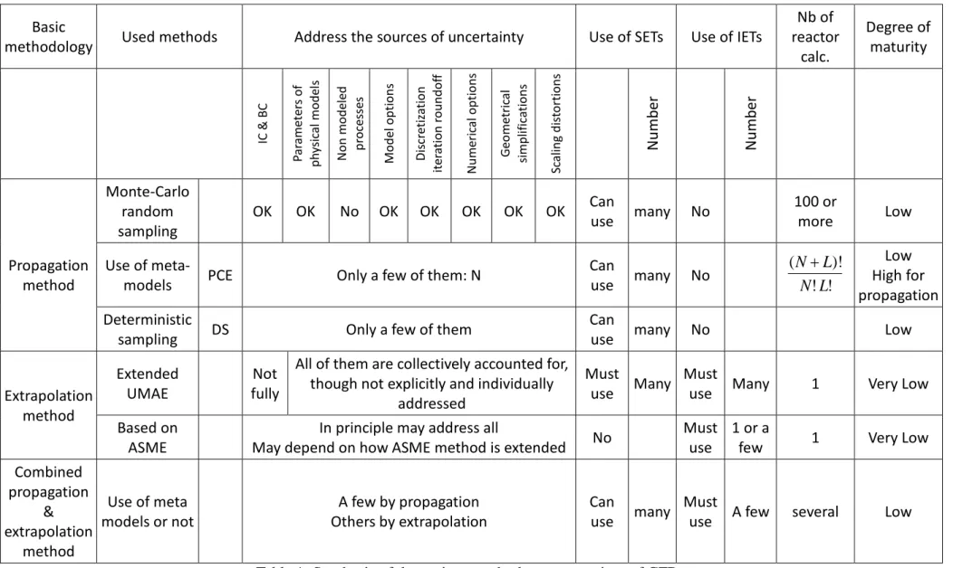
13 SYNTHESIS OF THE REVIEW - CONCLUSIONS AND RECOMMENDATIONS The use of single-phase CFD for safety of reactor requires that a general methodology is rigorously followed which includes a PIRT analysis, a scaling analysis and the scaling of some experiments, the selection of an appropriate CFD tool and of appropriate physical and numerical options, the building of an appropriate nodalization, the application of existing Best Practice Guidelines in the two previous steps, a comprehensive V&V program for the situation of interest, and the application of a mature Uncertainty Quantification method. Previous activities within WGAMA have elaborated BPGs and have identified assessment matrices for some selected safety issues but the lack of a consolidated uncertainty method is the main limitation for CFD application to a safety demonstration.
A review of existing work in this field was made but very limited information was found on CFD UQ applied to nuclear reactor safety analysis. The various methods are synthesized in the Table 1.
The main reactor issues where CFD UQ methods are expected to be applicable in short and medium term are mixing problems (temperature, boron concentration, H2 concentration, etc.) with or without density effects.
21
The two types of methods developed and used for UQ of system codes may be extended to CFD with some adaptation:
• The methods based on the propagation of input parameters uncertainty • The methods based on the extrapolation of accuracy
However the adaptation is still in progress and there is a rather limited feedback from a few first applications. Some preliminary observations and conclusions may be given:
• The various sources of code prediction uncertainty include initial and boundary conditions, physical properties, parameters of the physical models, non modelled physical processes, numerical models, numerical solution errors, simplifications of the geometry, possible chaotic behavior, extrapolation beyond the validated domain. • The propagation method with Monte-Carlo sampling is applicable to CFD even with a
large number of input uncertain parameters but it may lead to prohibitive CPU cost in some reactor issues.
• The use of deterministic sampling rather than random sampling may be a cheaper alternative for propagation methods.
• The use of meta-model may be a somewhat cheaper alternative for propagation methods when the number of input uncertain parameters is low. When used at first order, it is close to the DS method in terms of required number of calculations.
• The determination of uncertainty due to physical models is not straightforward for propagation methods. For example, uncertainty on parameters of turbulence models may depend strongly on the type of flow configuration.
• The extrapolation methods have the advantage of taking benefit from integral effect tests which are often designed to study the safety issue of interest. They require less CPU cost than Monte-Carlo propagation methods. However a preliminary work is necessary with the calculation of many SETs and IETs. Moreover, it still has to be proved that a pure extrapolation method like UMAE can be adapted or extended to CFD. • The uncertainty due to numerics compared to other sources of uncertainty is relatively
more important than for system codes and requires a special attention. Methods for numerical error evaluation exist but they may fail or be difficult to use in practical applications.
• The validation of the CFD tool on scaled IETs relative to a situation of interest seems to be mandatory either in the V&V process or in both V&V and UQ steps.
• A combination of propagation and extrapolation techniques may be a reasonable compromise in order to limit the number of calculations and the CPU cost.
• The CPU cost is still the main hindrance to the CFD application but the continuous progress of computer efficiency will progressively erode this obstacle.
The maturity of all the reviewed methods is medium, low or very low, some of them need extensions or adaptations and an extensive testing and all need to be benchmarked. Benchmarking is required. The main recommendations are:
• An effort should be devoted to the determination of uncertainty due to physical models for propagation methods. Methods should be tested following what has been done in the PREMIUM (www.oecd-nea.org) benchmark for system codes.