Modelling coronary blood flow using a non Newtonian fluid model : fractional flow reserve estimation

HAL Id: tel-02430901

https://tel.archives-ouvertes.fr/tel-02430901v3

Submitted on 22 Jun 2020

HAL is a multi-disciplinary open access

archive for the deposit and dissemination of sci-entific research documents, whether they are pub-lished or not. The documents may come from teaching and research institutions in France or abroad, or from public or private research centers.

L’archive ouverte pluridisciplinaire HAL, est destinée au dépôt et à la diffusion de documents scientifiques de niveau recherche, publiés ou non, émanant des établissements d’enseignement et de recherche français ou étrangers, des laboratoires publics ou privés.

fluid model : fractional flow reserve estimation

Keltoum Chahour

To cite this version:

Keltoum Chahour. Modelling coronary blood flow using a non Newtonian fluid model : fractional flow reserve estimation. Modeling and Simulation. COMUE Université Côte d’Azur (2015 - 2019); Université Mohammed V (Rabat), 2019. English. �NNT : 2019AZUR4098�. �tel-02430901v3�

modèle de fluide non Newtonien: estimation de la fraction de

réserve fluide

Keltoum CHAHOUR

Laboratoire J.A. Dieudonné

Présentée en vue de l’obtention du grade de docteur en mathématiques de

l’université Côte d’Azur et de l’université Mohammed V de Rabat.

Dirigée par: Abderrahmane Habbal /

Rajae Aboulaich.

Soutenue le: 02 Décembre 2019.

Devant le jury, composé de:

Rajae Aboulaich, Professeur EMI.

Soumaya Boujena, Professeur Université Hassan II. Abderrahmane Habbal, MDC HC HDR, UCA.

Olivier Pantz, Professeur LJAD, UCA.

Vitaly Volpert, Directeur de recherche CNRS.

Nejib Zemzemi, CR Carmen Team, INRIA Bordeaux. Mohamed Ziani, MDC HDR Université Mohammed V.

l’aide d’un modèle de fluide non Newtonien:

estimation de la fraction de réserve fluide

Jury:

Président du jury

Olivier Pantz, Professeur, Laboratoire de Mathématiques,

Université Côte d’Azur, Nice.

Rapporteurs

Soumaya Boujena, Professeur, Université Hassan II-Faculté des

Sciences Ain Chock, Casablanca, Maroc.

Vitaly Volpert, Directeur de recherche au CNRS, Institut

Camille Jordan, UMR 5208 CNRS, University Lyon 1 (absent).

Examinateurs

Mohamed Ziani, MDC HDR, Université Mohammed V, Rabat,

Maroc.

Je tiens à remercier toutes les personnes qui ont contribué à l’aboutissement de cette thèse et qui m’ont aidé à mener à bien mes travaux de recherche. Tout d’abord, je voudrais exprimer ma profonde gratitude envers mes deux directeurs de thèse. Je remercie chaleureusement Professeur Rajae ABOULAICH pour sa gentillesse, sa disponibilité, son aide et soutien sur les plans personnels et professionnels. C’est grâce à elle que j’ai pu découvrir le domaine des biomathématiques. Je souhaite aussi exprimer ma reconnaissance envers Professeur Abder-rahmane HABBAL pour sa confiance, sa gentillesse, et sa disponibilité. Je remercie égale-ment Docteur Chérif Abdelkhirane de m’avoir proposé un sujet aussi riche et intéressant et d’actualité. C’est grâce à son expertise clinique que j’ai pu cerner les différents aspects liées à la circulation cardiovasculaire. Ses conseils et orientations m’ont aidé à améliorer la qualité de mon travail.

Je remercie ensuite Professeur Soumaya BOUJENA et Professeur Vitaly VOLPERT d’avoir accepté d’être rapporteurs de cette thèse. Je les remercie pour l’attention et le temps qu’ils ont accordés à mon manuscript. Mes remerciements s’adressent également à Professeur Olivier PANTZ, Professeur Nejib ZEMZEMI et Professeur Mohamed ZIANI de m’avoir fait l’honneur d’accepter de participer au jury de cette thèse.

Je remercie également l’équipe CARMEN de l’INRIA de Bordeaux de m’avoir donné l’opportunité d’effectuer différents stages au cour de cette cotutelle. Particulièrement Mr. Nejib ZEMZEMI pour les collaborations fructueuses sur différentes questions.

Je remercie aussi le laboratoire Jean Alexandre Dieudonné pour m’avoir accueilli dans ses locaux et donné l’accès à ses ressources de calcul. Mes sincères remerciements vont aussi aux deux ingénieurs informatiques du laboratoire: Mr. Jean-Marc LACROIX et Mr. Roland RUELLE pour leur accueil et leur accompagnement tout au long de la phase du cal-cul parallèle.

Finalement je remercie l’équipe ACUMES et l’INRIA Sophia Antipolis pour m’avoir ac-cueilli dans ses locaux et donné l’accès à ses ressources. Je remercie particulièrement Mr. Mickael BINOIS pour la collaboration fructueuse.

Je dédie ce modeste travail et ma profonde gratitude à ma très chère maman et mon très chère père.

Dans cette thèse, nous explorons la possibilité d’une évaluation virtualle des sténoses à travers la simulation de l’index de la réserve coronaire - appelée FFR en anglais - qui est un outil indispensable mais contraignant lors du diagnostic. Tout d’abord, nous utilisons un modèle d’écoulement 2D non Newtonien, puis un modèle d’interaction fluide structure faiblement couplé pour établir une étude préliminaire des principales caractéristiques de l’écoulement dans une portion sclérosée. Nous introduisons ensuite une méthodologie pour estimer la FFR virtualle par analogie avec le dispositif médical. Le capteur FFR a été, dans un premier lieu, considéré non physique (intégré au domaine d’écoulement). Nous avons mené différents tests numériques pour relever les facteurs affectant la FFR virtualle et présenté son profil par rapport aux différents paramètres considérés pour la lésion. Deuxièmement, nous présentons deux géométries réalistes : un arbre coronaire gauche - en 2D - obtenu à partir de la segmentation d’une image angiographique et une bifurcation en 3D. Nous définissons des modèles d’écoulement généralisés à l’intérieur des deux géométries et considérons que la paroi artérielle est rigide. La présence de plusieurs sorties dans ces nouvelles géométries nous a conduit à utiliser un nouveau type de conditions aux limites. A l’entrée, nous pro-posons une fonction bi-sinusoïdal s’approchant du profil de vitesse sanguine enregistré pour un arbre coronaire gauche. En ce qui concerne les sorties du domaine, nous considérons un modèle Windkessel à 2 éléments. Nous avons mené une étude comparative entre le mod-èle de Navier Stokes et le modmod-èle non Newtonien considéré et entre les conditions limites de sorties libres et le modèle Windkessel présenté en 2D et défini le flux à l’intérieur de l’arbre de bifurcation 3D. Nous calculons également la FFR virtual de deux lésions artifi-cielles ajoutées à l’arbre coronaire et démontrons que l’angiographie seule ne suffit pas pour évaluer la sévérité de la sténose. Troisièmement, nous étudions - par modélisation 2D et 3D - une des raisons possibles de la dérive de pression pendant la mesure de la réserve coronaire FFR, représentée par la position et la configuration arbitraires du capteur de pression. Le capteur est considéré durant cette étude extrinsèque au domaine de l’écoulement. Nous con-sidérons les mêmes modèles de flux non Newtoniens que précédemment. En 2D, le capteur FFR est assimilé à un disque avec une position variable incorporée dans l’arbre coronaire gauche. Alors que le domaine 3D correspond à une portion artérielle sclérosée à laquelle

tique basé sur la loi de Hooke. À l’aide d’un processus gaussien, nous modélisons le FFR en fonction des variables du capteur - et deux autres variables de la lésion - nous effectuons un ensemble d’expériences correspondant à l’espace d’hypercube considéré. Les données 2D indiquent une bonne précision pour la prédiction de FFR tandis que les données 4D con-firment le fait que les micro-cathéters avec des diamètres importants surestiment la gravité des lésions. Les résultats obtenus démontrent que la dérive qui se produit en raison de la configuration variable du dispositif FFR peut induire en erreur lors de la classification de la sténose. Tous les algorithmes de résolution et les outils de simulation ont été implémentés sous le logiciel FreeFem++. Le besoin de plus d’espace mémoire pour les simulations 3D nous a conduit à adopter une stratégie de résolution parallèle utilisant FreeFem+++ MPI et le solveur MUMPS.

Mots clés: Écoulement non Newtonien; Fraction de réserve coronair; Athérosclérose; Processus gaussiens; Dérive.

In this thesis, we explore the possibility of virtual coronary stenosis assessment, through the simulation of Fractional Flow Reserve (FFR) measurement, that is an indispensable but bind-ing tool durbind-ing diagnosis. First, we use a 2D non Newtonian flow model, and later a weakly coupled FSI model to make a preliminary study of the main features of flow over a stenotic coronary arterial portion. We then introduce a methodology to estimate the virtual FFR in analogy with the clinical device. The FFR device was considered non-physical (integrated to the flow domain) at a first place. We led different experiments to enumerate the factors affecting the virtual FFR and computed its profiles with respect to different lesion’s parame-ters. Second, we consider two realistic geometries: a 2D left coronary tree obtained from the segmentation of an angiography image and a 3D bifurcation tree. We define generalized flow models inside the two geometries and consider the arterial wall to be rigid. The presence of several outlets in these new geometries led us to define a new type of boundary conditions. For the inlet, we propose a bi-sinusoïdal function approaching the velocity profile recorded inside a left coronary tree. For the outlets, we implement a 2 element Windkessel model. We led a comparative study between Navier Stokes and the flow model considered and between free outlets boundary conditions and Windkessel model in 2D and define the flow inside the 3D bifurcation tree. We also compute the virtual FFR of two artificial lesions added to the coronary tree and demonstrate that angiography alone is not enough to evaluate the severity of stenosis. Third, we investigate - through 2D and 3D modelling - one possible reason of pressure drift during FFR measurement, that is the arbitrary position and configuration of the FFR device, considered during this study extrinsic to the flow domain. We consider the same non Newtonian flow models as previously. In 2D, the FFR device is assimilated to a disk with a variable position incorporated inside the left coronary tree. While the 3D do-main corresponds to a diseased arterial portion to which we introduce a deformed 3D tube (wire+sensor) with a given length and coefficient of bending. The bending effect of the tube is obtained thanks to an elastic problem based on Hooke’s law. Using a Gaussian process, we model the FFR depending on these variables - and two additional stenosis variables later - we perform a set of samples corresponding to the design space considered. The 2D data indicates a good accuracy for FFR prediction while the 4D data emphasis the fact that

mi-stenosis misclassification. All resolution algorithms and simulation tools were implemented under FreeFem++ software. The need of more space memory for 3D simulations led us to adopt a parallel resolution strategy using FreeFem++ MPI and MUMPS solver.

Key words: Non Newtonian flow; Fractional Flow Reserve; Atherosclerosis; Gaussian processes; Drift.

1 Introduction 15

2 Preliminary 19

2.1 Clinical context . . . 20

2.1.1 Atherosclerosis . . . 20

2.1.2 Fractional Flow Reserve . . . 21

2.1.3 Blood circulation in the heart . . . 21

2.1.4 FFR devices: FFR guidewire vs microcatheter . . . 24

2.2 Mathematical context . . . 25

2.2.1 Blood flow modelling . . . 25

2.2.2 Virtual Fractional Flow Reserve . . . 27

3 Virtual Fractional Flow Reserve (VFFR) computation 29 3.1 Introduction . . . 30

3.2 Fractional flow reserve . . . 30

3.3 Generalized non newtonian flow model . . . 33

3.4 Numerical results . . . 36

3.4.1 The case of single stenosis . . . 36

3.4.2 Mutli-stenosis case . . . 40

3.5 Coupling scheme: fluid-structure interaction . . . 41

3.6 Conclusions . . . 43

4 Blood flow simulation in realistic domains using Windkessel boundary condi-tions 45 4.1 Introduction . . . 46

4.2 Mathematical modelling . . . 47

4.2.1 Domain definition: 2D image segmentation . . . 47

4.2.2 Coronary blood flow model . . . 47

4.2.3 Boundary conditions : Inlet / Outlets . . . 49

4.2.5 Fractional flow reserve (FFR) . . . 53

4.3 Numerical results . . . 54

4.3.1 Fractional Flow Reserve (FFR) computation . . . 56

4.3.2 Discussion . . . 58

4.4 3D modelling . . . 58

4.4.1 Details about the flow model and boundary conditions . . . 59

4.4.2 Details about the numerical simulation . . . 60

4.4.3 3D results . . . 62

4.5 Drift quantification . . . 64

4.5.1 Conclusion . . . 64

5 Fractional flow reserve prediction using gaussian processes 66 5.1 Introduction . . . 67

5.2 Quantification of the sensor position impact on the FFR value: 2D case . . 69

5.2.1 Sensor position: effect on the virtual FFR . . . 69

5.2.2 Numerical results: flow distributions . . . 70

5.2.3 FFR variation corresponding to both directions . . . 72

5.3 Quantification of the sensor position impact on the FFR value: 3D cases . . 75

5.3.1 Sensor bending problem . . . 75

5.3.2 3D Flow model for simulations . . . 77

5.3.3 Details about numerical simulation . . . 78

5.3.4 Some 3D results . . . 80

5.3.5 Gaussian process modelling . . . 80

5.3.6 Comparing FFR issued from virtual sensor to that from a physical sensor . . . 89

5.4 Conclusions . . . 91

2.1 Angioplasty : stent implantation, [37] . . . 20 2.2 The right and left coronary arteries of the heart. . . 22 2.3 Systole and diastole refer respectively to the contraction and relaxation of

the two right or left ventricles of the heart. . . 23 2.4 Sections of piezo-electrical sensor, microcatheter and optical sensor from left

to right respectively. Left, standard wire core surrounded by thin transmis-sion and ground wires. Center, ultra thin microcatheter using optical fiber: sensor housing + guidewire. Right, nitinol cobalt chromium wire around central optical fiber. . . 25 3.1 Left, representatif schema of the invasive FFR technique [16]. Right, a

typ-ical example of FFR measurement. Automated calculation of FFR corre-sponds to the ratio of mean distal coronary pressure (green) to mean aortic pressure (red) during maximal hyperemia, see [15]. . . 31 3.2 Considered geometry for the problem. . . 35 3.3 Left, velocity and pressure field with Navier Stokes equation at time t = 0.3s.

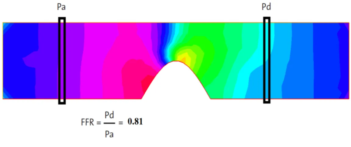
Right, velocity and pressure field with the generalized flow model at time t= 0.3s . . . 37 3.4 FFR calculation. In this case, the degree of stenosis is equal to 40% and the

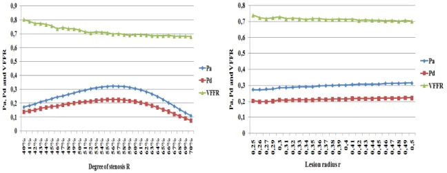
VFFR is equal to 0.81. . . 37 3.5 VFFR variation during 5 cardiac cycles for a lesion with 75% stenosis. . . 38 3.6 Left, Pa, Pdand VFFR variation according to the degree of stenosis R. Right,

Pa, Pdand VFFR variation according to the lesion radius δ . . . 38

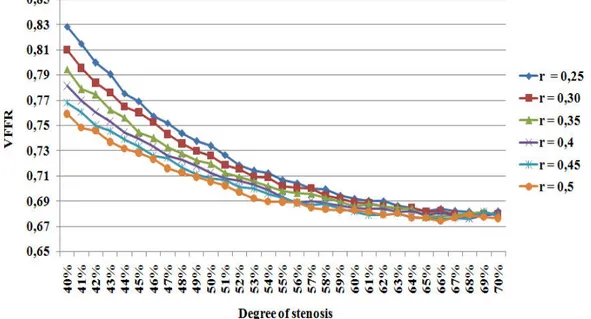
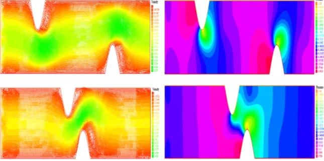
3.7 VFFR variation for lesions with different radius according to the degree of stenosis. . . 39 3.8 Top, velocity and pressure field corresponding to identic lesions of 40%

stenosis, with a spacing ’a’ of 1.5 cm. Bottom, velocity and pressure field with a spacing ’a’ of 0.5 cm . . . 40

3.9 Left, Pa, Pd and VFFR variation according to the degree of stenosis R in the

case of multiple stenoses. Right, Pa, Pd and VFFR variation according to the

lesion radius δ in the case of multiple stenosis. . . 41 3.10 VFFR variation in the case of two identic lesions, with different spacings

according to the degree of stenosis. . . 41 3.11 Pressure profil with the fluid-structure interaction model. . . 42 3.12 Left, Pa, Pd and VFFR variation according to the degree of stenosis R (D

defined in equation 3.11 using the fluid-structure interaction model. Right, Pa, Pd and VFFR variation according to the lesion radius δ using the

fluid-structure interaction model. . . 42 3.13 VFFR variation using the fluid-structure interaction model according to the

degree of stenosis. . . 43 4.1 From left to right: The original angiography image, the coronary tree of

in-terest is framed with red. The Black and white original image. The resulting multi-stenotic coronary tree. . . 48 4.2 The 2D geometry considered. Arrows indicate the isoline orientation. . . . 49 4.3 Left, spline function approaching left coronary blood flow. Right, the flow

function prescribed at the inlet I(t). . . 50 4.4 Windkessel electrical analogy. . . 52 4.5 FFR calculation. The mutli-stenotic coronary tree contains two lesions: 56%

stenosis and 68% stenosis. . . 53 4.6 From top to bottom: Velocity and pressure fields at t = 0.59s (peak diastole)

using Windkessel model, free pressure outlet boundary conditions and mixed outlet boundary conditions (as defined in the paragraph above) respectively. 55 4.7 3D domain used for simulations. . . 59 4.8 Left to right, 2D slices of the initial velocity and pressure fields for simulations. 61 4.9 3D mesh of the coronary tree used for simulations. . . 61 4.10 Top, pressure fields inside the healthy coronary tree at peak systole (left) and

peak diastole (right). Bottom, corresponding velocity fields. . . 62 4.11 Top, pressure fields inside the diseased coronary tree at peak systole (left)

and peak diastole (right). Bottom, corresponding velocity fields. . . 63 5.1 Main elements of FFR measurement: guiding catheter, pressure guide and

distal sensor. . . 67 5.2 Left, a simplified 3D model of the device wire+sensor. Right, image

corre-sponding to an optical FFR device from the market. . . 69 5.3 Distal sensor displacement according to the normal and tangential positions. 69

5.4 Top, velocity field using generalized fluid model at peak systole (left) and peak diastole (right). Bottom, velocity field using Navier Stokes at peak systole (left) and peak diastole (right). . . 71 5.5 Velocity distributions near stenosis with the two flow models at different

times of the cardiac cycle. Left, top peak diastole - generalized flow model; bottom peak systole generalized flow model. Right, top peak diastole -Navier Stokes; bottom peak systole - -Navier Stokes. . . 72 5.6 Left, comparison between FFR values for Navier Stokes and Non Newtonian

flow model obtained by moving the sensor in the normal direction. Right, comparison between FFR values for Navier Stokes and Non Newtonian flow model obtained by moving the sensor in the tangential direction. The grey area represents critical FFR values. . . 73 5.7 Left, comparison between FFR values for Navier Stokes and Non

Newto-nian flow model combined with free outlets or Windkessel BC obtained by moving the sensor in the normal direction. Right, comparison between FFR values for Navier Stokes and Non Newtonian flow model combined with free outlets or Windkessel BC obtained by moving the sensor in the tangential di-rection. . . 74 5.8 3D configuration of the pressure guide + sensor. . . 76 5.9 Position of reference of the pressure sensor and the two new configurations

due to bending. . . 76 5.10 The diseased arterial portion + the FFR guide/sensor. . . 77 5.11 Left, blood velocity at three different times of the cardiac cycle. Right,

cor-responding blood pressure fields. . . 81 5.12 Predicted FFR given by GP regression. Designs are marked by points (resp.

triangles) for the training (resp. testing) set used later. The dashed lines and dotted box are used later for uncertainty quantification. Left:predictive mean of the FFR values given by the GP. Right: corresponding predictive standard deviation. . . 85 5.13 Left: predicted FFR versus simulation, the black points depict the mean

prediction while the segments denote the 95% prediction intervals. Right: boxplot of FFR values for random position along the segments and box rep-resented in Figure 5.12. The median is reprep-resented by the thick line while the box is defined by the lower and upper quartiles. . . 86 5.14 3D view of the statistical predictor. . . 86

5.15 Left: velocity streamlines corresponding to sample 49: L = 3.712, coe f = 55.08 and FFR = 0.4043. Right: velocity streamlines of sample 54: L = 3.86, coe f = −59.0136 and FFR = 0.38. . . 87 5.16 Velocity isolines at peak systole. The shadowed tube illustrates the virtual

device sensor/guide. . . 90 5.17 Left, velocity isolines at peak systole. Right, velocity isolines at peak

4.1 FFR values for both lesions correponding to the two flow models and the different outlet boundary conditions. The two mesh files presented in figure 3.5 were used for these calculations. . . 56 4.2 FFR values for the second lesion at 5 different cardiac cycles, for different

values of the meshsize. The same value of time step was adopted for all simulations dt = 5 × 10−3_{. FFR is the value for the cardiac cycle while}

FFRais the average FFR value. . . 57

5.1 Two parameters design experiments: parameters and corresponding FFR val-ues . . . 84 5.2 Four parameters design experiments: parameters and corresponding FFR

Introduction

Cardiovascular diseases (CVDs) are the major cause of death globally, killing more than 17.9 million worldwide, according to WHO (World Health Organization). Therefore, 31% of total global mortality is due to cardiovascular diseases. An estimated 7.4 million are due to coronary heart disease and 6.7 million to a stroke (2015). Atherosclerosis is one of the most common pathologies that lead to stroke. It is a chronic inflammatory disease that af-fects the entire arterial network and especially the coronary arteries. It is an accumulation of fat cells and lipids over the arterial surface due to a dysfunction of the endothelial layer (finer superior layer of blood vessel). The grassy deposit is commonly known as plaque or lesion in clinical context. The objective of clinical intervention in this case is to establish a revascularization, in order to allow the blood to circulate in a normal way among the diseased vessel. The first problem we were interested in during this thesis was the multidisciplinary optimization of drug-eluting stents. The objective was to find the optimal design (topology and characteristics) of the stent which ensures a permanent enlargement of the damaged por-tion while reducing the risks induced by the immune reacpor-tions of the arterial wall (restenosis, thrombosis ...). In order to have a good understanding of the pathology and the clinical pro-cesses associated with it, a contact with practitioners in the field of interventional cardiology was required. Here we tried to have contact with AMCAR, the Moroccan association of cardiology in Casablanca. They put us in contact with Dr. Chérif Abdelkhirane, a specialist in stenting and interventional cardiology, head chief of the clinical center Cardiology Maarif in Casablanca at the time, and now head of the department of Interventional Cardiology, Clinique des spécialités Achifaa, Casablanca, Morocco. From the very first discussions, we could realize that what matters the most from a cardiologist’s point of view is to ensure a better revascularization. While the stent design, according to them, is not determinant of the post-intervention results. Especially that the stents available in the market are enough sophis-ticated. That is why he suggested a new problematic for the thesis. Indeed, revascularization is based on the principle of remedying ischemia, that is the decrease or the interruption of

oxygen supply to the organs. This anomaly - ischemia- is attenuated by the presence of more than one lesion (multivariate patients), which can lead to several complications. The key to a good medical intervention is establishing a good diagnosis. During the diagnosis phase, the cardiologist uses several techniques for decision making, among which angiography is the most intuitive. Angiography is an X-ray technique to visualize the inside ( the lumen ) of blood vessels in order to identify vessel narrowing: stenosis. Despite its widespread use, angiography is often imperfect in determining the physiological significance of coro-nary stenosis. The clinical decision is based on the degree of stenosis, that corresponds to the plaque’s height over the diameter of reference of the diseased arterial portion. If the prob-lem remains simple for minimal lesions (≤ 40%) or very severe ( ≥ 70%), a very important category of intermediate lesions must benefit from a hemodynamic evaluation in order to determine the outcomes of revascularization. Fractional Flow Reserve (FFR) can be a better alternative in this case.

In the first chapter, we give the necessary elements to define the context of our work. Firstly, some clinical precisions about the pathology of atherosclerosis and the methods of diagnosis and treatment. Secondly, we establish a state of the art of the works that were interested in the simulation of blood flow.

In the second chapter of this thesis, we provide a first estimation of a virtual non-invasive Fractional Flow Reserve (VFFR). We present a preliminary study of the main features of flow over a stenosed coronary arterial portion, in order to enumerate the different factors affecting the VFFR, and to emphasis considering other parameters than the degree of stenosis to judge the severity of a coronary lesion. In particular, the lesion radius, as demonstrated by the clinical study given in [17]. We adopt a non Newtonian flow model inside a 2D simplified domain assumed to be rigid in a first place, corresponding to the artery geometry in maximum vasodilation. In a second place, we consider a simplified weakly coupled FSI model in order to take into account the infinitesimal displacements of the upper wall. No large displacements are taken into account. A 2D finite element solver was implemented using Freefem++. We computed the VFFR profiles with respect to different lesion parameters and compared the results given by the rigid wall model to those obtained for the elastic wall one.

In the third chapter, we adopt realistic domains, issued from reconstructed coronary trees. Two geometries were adopted: the first one corresponds to a 2D left coronary tree, issued from an angiography, to which we included two artificial lesions of different degrees. The second one is a 3D bifurcation to which we add an artificial lesion. We used the same generalized fluid model as in the first chapter with a Carreau law in 2D and 3D, but addressed a special concern to boundary conditions. We use a coupled multidomain method based on a 2 element Windkessel model as outlet boundary condition. At the inlet, instead of using a wave form function, we opted for a double-sinusoïdal profile similar to flow data curves

from a left coronary tree. We introduce our methodology to quantify the virtual FFR, and lead several numerical experiments. We compare FFR results in 2D for Navier Stokes versus generalized flow model, and for Windkessel versus free outlets boundary conditions. In the fourth chapter, we try to study the impact of the pressure wire design and configuration on the computed FFR value, in order to quantify the uncertainties induced in the measure. Inside a 3D domain modelling a diseased coronary portion, we insert a microcatheter-design sensor to capture the proximal and distal pressures. We use a generalized 3D fluid model and we run different simulations to enumerate the effect of the sensor’s configuration on the estimated FFR. Gaussian processes are then used to provide a statistical model to predict the FFR value.

Publications

• K.Chahour, R.Aboulaich, A.Habbal, C.Abdelkhirane and N.Zemzemi “Numerical sim-ulation of the fractional flow reserve (FFR)”, Math. Model. Nat. Phenom. 13 (2018). • K.Chahour, R.Aboulaich, A.Habbal, C.Abdelkhirane and N.Zemzemi “Virtual FFR

quantified with a generalized flow model using Windkessel boundary conditions: Ap-plication to a patient-specific coronary tree”, Computational and Mathematical Meth-ods in Medicine (submitted in August 2019).

• K.Chahour, A.Habbal, M.Binois, R.Aboulaich and C.Abdelkhirane “Drift quantifica-tion during fracquantifica-tional flow reserve measurement using Gaussian processes” (final stage of writing).

• C. Bonnet, K. Chahour, F. Clément, M. Postel, R.Yvinec “Multiscale population dy-namics in reproductive biology: singular perturbation reduction in deterministic and stochastic models ”, ESAIM PROCS (accepted in July 2019).

Communications in international conferences

• October 2018 – BIOMATH 2018: Hassan II University, Mohammedia Morocco. “Re-alistic blood flow simulation in a 2D reconstructed coronary tree“

• June 2018 – PICOF’18: American University of Beirut, Beirut, Lebanon. “Simulation of blood flow in a stenosed artery and fractional flow reserve computation“

• October 2017 – ICAM’17: Faculty of science and technology Taza, Morocco. “Nu-merical simulation of the fractional flow reserve (FFR)”

Preliminary

Abstract

Blood flow simulation inside diseased coronary arteries is a crucial task before computing the virtual Fractional Flow Reserve (FFR). In this preliminary chapter, we highlight some clinical aspects of coronary blood circulation, atherosclerosis and the invasive FFR measure-ment. On the other hand, we establish a state of the art of the works in applied mathematics that investigated in this view in order to enumerate the elements to be considered to better modelize our problem.

2.1

Clinical context

2.1.1

Atherosclerosis

Atherosclerosis is a chronic inflammatory disease that affects the entire arterial network and especially the coronary arteries. It is an accumulation of fat cells and lipids over the arterial surface due to a dysfunction of the endothelial layer (finer superior layer of blood vessel). The grassy deposit is commonly known as plaque or lesion in clinical context. The objective of clinical intervention in this case is to establish a revascularization, in order to allow the blood to circulate in a normal way among the diseased vessel. Different angioplasty tech-niques can be envisaged, among which implantation of stents is the most widespread. The cardio-stent is a small metallic tube that has generally a periodic design composed by a re-peated pattern. It acts like a scaffold to support the inside of the diseased portion of artery. The intervention, called stent implantation, consists on introducing a stent into the damaged arterial portion. The stent is placed over a balloon catheter, that is placed over a guide wire, in order to be brought into the site of the plaque. Once there, the balloon is inflated and the stent expands to the size of the artery and holds it open. The balloon is then deflated and removed while the stent stays in place.

Figure 2.1: Angioplasty : stent implantation, [37]

The physical characteristics as well as the geometric design of the stents in industries involved so that this last could have an optimal performance once placed on the site of atherosclerosis. Combining different criterias: flexibility, manageability, opacity, inoxid-ability, bio-compatibility... Two potential post-stenting risks are intra-stent restenosis and thrombosis, see [52]. Restenosis is due to an excessive tissue proliferation in the luminal surface of the stent, leading to a reduction in lumen diameter after coronary intervention. Thrombosis is an acute consequence to restenosis in the case where a part of cells is liber-ated from the lumen surface to form an occlusion and lead to stroke. In order to reduce these

risks, a new generation of drug-eluting stents has appeared. A drug eluting stent is nothing else but a stent covered by a fine layer of polymer containing an antiproliferative substance.

2.1.2

Fractional Flow Reserve

Fractional Flow Reserve (FFR) is a lesion specific, physiological index determining the hemodynamic severity of intracoronary lesions. FFR can accurately identify lesions respon-sible for ischemia which in many cases would have been undetected or not correctly assessed by angiography alone. FFR is defined as the maximum achievable blood flow in stenotic coronary artery (Pd) divided by maximum blood flow in the same artery without stenosis (Pa). FFR has a unique normal value of 1.0 in healthy coronary artery. An FFR = 0.80 is commonly accepted as the threshold below which a lesion is considered ischemia causing. The invasive FFR measurement is established during maximum hyperemia, administrated by adenosine stimulus. It is only at maximal hyperemia that resistance is minimal and that flow develops a linear relationship to pressure, a vital prerequisite for the FFR equation to hold true. Not achieving maximal hyperaemia will overestimate the FFR value and therefore underestimate the true severity of a coronary stenosis. More technical details about the FFR clinical test and the FFR device will be given in the next section 2.1.4. As demonstrated by multiple clinical studies, particularly FAME study [11], FFR is the current gold stan-dard to improve clinical decision making in the case of coronary stenosis. Using a patient data collected from more than 20 medical centers in the united states and Europe, patients were randomly assigned to undergo with stent implantation guided by angiography alone or guided by FFR measurement in addition to angiography, see [11]. The conclusion of FAME study is that the FFR improved the clinical outcomes and contributed in reducing the mortality rate.

2.1.3

Blood circulation in the heart

Bloodis a complex mixture of blood cells suspended in blood plasma. Plasma, which consti-tutes 55% of blood fluid, is mostly water (92% by volume), contains proteins, lipoproteins, and ions by which nutrients and wastes are transported to the different organs. Red blood cells comprising approximately 40% of blood by volume are small semisolid particles. They are responsible of increasing the viscosity of blood that is four times more viscous than wa-ter. Blood does not exhibit a constant viscosity at all flow rates and thus has a non-Newtonian behavior especially in the microcirculatory system, such as the coronary arteries. However, in large arteries like the aorta, blood behaves in a Newtonian fashion, and the viscosity can be considered constant. In this work, we give a special concern to the coronary arteries.

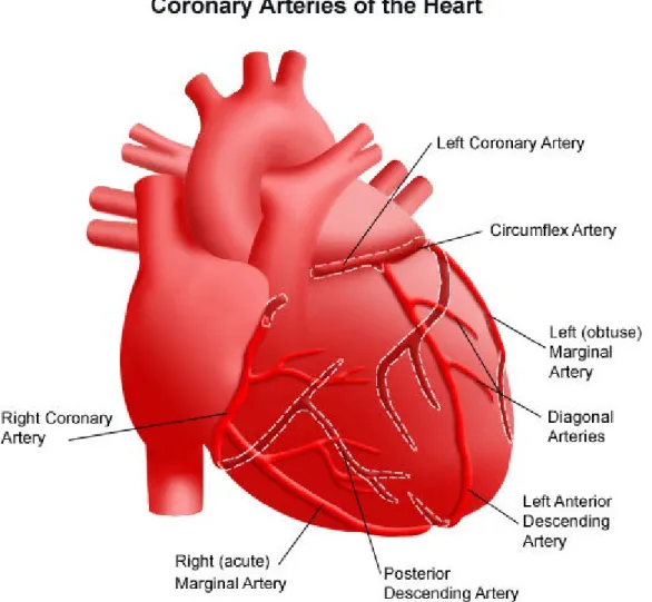
Coronary arteries, see figure 2.2 constitute the vascular system that supplies oxygen to the heart muscle, called myocardium. The aorta branches off into two main coronary blood ves-sels. These coronary arteries glued to the heart muscle branch off themselves into smaller arteries and capillaries that transport oxygen-rich blood. The right coronary artery supplies blood mainly to the right side of the heart. The right side of the heart is smaller because it pumps blood only to the lungs. The left coronary artery, which branches into the left anterior descending artery and the circumflex artery, supplies blood to the left side of the heart. The left side of the heart is larger and more muscular because it pumps blood to the rest of the body.

Figure 2.2: The right and left coronary arteries of the heart.

Blood flow and pressure are unsteady. The cyclic nature of the heart pump creates pul-satile conditions in all arteries. The heart ejects and fills with blood in alternating cycles called systole and diastole with a frequency of 75 beats per minute. Blood is pumped out of the heart during systole while the heart rests during diastole, and no blood is ejected. A

heart cycle lasts about 0.8 seconds, systole occupies the third while diastole occupies the two thirds.

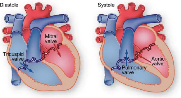
During systole, intramuscular blood vessels are compressed and twisted by the contract-ing heart muscle and blood flow to the left ventricle is at its lowest. The force is greatest in the sub-endocardial layers where it approximates to intramyocardial pressure, figure 2.3. In systole intramyocardial blood is propelled forwards towards the coronary sinus and ret-rogradely into the epicardial vessels, which act as capacitors. Flow resumes during diastole when the muscle relaxes. The coronary perfusion pressure is the difference between the aor-tic diastolic pressure and left ventricular end-diastolic pressure (LVEDP). Phasic changes in blood flow to the right ventricle are less pronounced because of the lesser force of contrac-tion.

Figure 2.3: Systole and diastole refer respectively to the contraction and relaxation of the two right or left ventricles of the heart.

Central venous pressure may be a more appropriate choice for downstream pressure to calculate the right-sided coronary perfusion pressure. Pressure and flow have characteristic pulsatile shapes that vary in different parts of the arterial system, as illustrated in Figure 2.3. The flow out of the heart is intermittent, going to zero when the aortic valve is closed. The aorta, the large artery taking blood out of the heart, serves as a compliance chamber that provides a reservoir of high pressure during diastole as well as systole. Thus the blood pressure in most arteries is pulsatile, yet does not go to zero during diastole. In contrast, the flow is zero or even reversed during diastole in some arteries such as the external carotid, brachial, and femoral arteries. These arteries have a high downstream resistance during rest and the flow is essentially on/off with each cycle. In other arteries such as the internal carotid or the renal arteries, the flow can be high during diastole if the downstream resistance is low.

The flow in these arteries is more uniform.

2.1.4

FFR devices: FFR guidewire vs microcatheter

Despite strong outcome records, FFR is still underutilized. Areas for improvement of FFR equipement technology fall into three categories:

1. signal stability that is the main reason of pressure drift; 2. wire handling characteristics and rapid placement.

3. use of multiple wires for complex or multi-vessel assessment.

For FFR measurement, two main technologies are commercially available [35] and [54]. On the one hand, pressure wire technology that involves a special 0.014 inches wire. There are two main types of pressure wires, the most commonly used is the piezo-electrical. In this kind of pressure wires, the sensor is located at the proximal end of the radiopaque flexible wire tip (about 3 cm long). The value measured by the Piezoelectric sensor is a dynamic pressure. The approach is the following: a thin membrane over a large base is used, ensur-ing that an applied pressure specifically loads the elements in one direction. Deformation of the crystal generates an electrical charge, which is transmitted along thin wires inside the guidewire. The main disadvantage of this type of sensors is the potential for signal in-terference at connector points. To overcome the limitations given above, and especially, to improve signal stability, a new generation of optical sensors has appeared. In this case, thin optical fibers are incorporated around a metal core (e.g nitinol, cobalt chromium). The dif-ference in pressure measurement resides in the way of measuring the membrane deflection, which is optical rather than electrical. As blood pressure increases, the membrane deflects inward, which induces a phase delay between two light beams created within the sensor assembly. It should be noticed that optical FFR wires demonstrated a much better signal stability than the piezoelectrical ones, and thus less drift during FFR assessment [?]. On the other hand, microcatheter technology that employs a low-profile catheter with a pressure sensor incorporating fibre-optic technology into the distal end, giving a profile comparable to 0.022 inches diameter at the lesion site. This new equipement is convenient and may over-come some of the limitations associated with conventional pressure wire systems. It may also be less prone to pressure drift since it utilizes an optical pressure sensor. However, the larger elliptic profile, see figure 2.4, is observed to produce an additive contribution to lesion severity -compared to other models of FFR devices- and as a result lower the measured FFR value [34].

Figure 2.4: Sections of piezo-electrical sensor, microcatheter and optical sensor from left to right respectively. Left, standard wire core surrounded by thin transmission and ground wires. Center, ultra thin microcatheter using optical fiber: sensor housing + guidewire. Right, nitinol cobalt chromium wire around central optical fiber.

2.2

Mathematical context

2.2.1

Blood flow modelling

Simulating blood flow in the arterial network - and in the coronary arteries in particular - is a highly complex task. Combining different mathematical disciplines: computational fluid dynamics, elasticity and domain reconstruction. The main difficulties can be resumed in the following:

• The bio-fluid complexity of blood, and the choice of the appropriate value or formula for the viscosity term. Moreover, whether we are in large or small arteries, the choice of a Non-Newtonian flow model or Navier Stokes is crucial as to the accuracy of the solutions obtained.

• Arterial vessel walls show a so called "bioviscoelastic" behavior C302. This property has two important effects. First, the arterial wall deformation is a function of the transmural pressure and the time. Hence the “history” of the wall has an effect on the current state, according to the considered scheme.

• The geometrical complexity of the arterial network. It consists of numerous vessel branches with different length, diameter and stiffness (compliance). There are also several bifurcations in the system. Furthermore, there is a noise introduced by the large displacements of the respiratory system, constantly in contact with the heart.

During the last decades fluid mechanics has become a powerful tool in the analysis of arterial blood flow. A flow and pressure wave starts from the heart to cross all major arteries in which it is damped, dispersed and reflected due to changes in vessel sizes, as well as the properties of the tissues and branches. The propagation of the blood wave in the different arteries creates small displacements of the arterial wall due to its elastic property. That said, a realistic reproduction of blood flow in the coronary arteries involves:

• Taking into account the fluid and the arterial wall particularity : On one hand, the choice of a Newtonian fluid model using the Navier Stokes equations for example, under certain conditions, or Non Newtonian. The work in [51] presents some recent developments in blood flow modelling and gives a special concern to the non Newto-nian properties of blood. In the case of sclerotic arteries, the problem becomes more complex. More details about the inflammatory process that initiates atherosclerosis are given in [50]. On the other hand, the choice of a fluid-structure coupling model that takes into account the interaction between the arterial wall and the blood. These 2D and 3D coupling models were presented in several papers [1] [2][3] [5] [8]. Among them [1] [2] introduced the presence of stenosis.

• The choice of suitable boundary conditions for the inlets and the outlets of the system: Various studies have tackled the problem of boundary conditions in the case of the blood flow [3] [4] [6] . These last, if they do not agree with the problem posed and its geometrical configuration can cause stability problems due to the creation of reverse flow, which does not correspond to the physical reality of the flow. Indeed, the difficulty resides in the fact of isolating a part of a network which is in fact closed, and in which the flow is periodic. The boundary condition at the inlet is often a sinusoïdal, parabolic or a spline function extracted from a medical data. At the outlet, the most common boundary condition are constant pressure or traction with a velocity profile. In the case of complex geometries, or 3D domains reconstructed from medical imag-ing, in which there are several evacuations, the condition at the outlet boundary must be chosen in order to avoid having inaccurate values of pressure and velocity. The best boundary conditions in the outlet for cardiovascular flow applications are not those which do not produce reflections, since reflections naturally come from the change in the vessels caliber, bifurcations, variation in the properties of the wall ... etc, which produces a resistant effect at the exit of the large vessels. For this reason, the bound-ary conditions based on the impedance and resistance models are the most adapted to incorporate this reflected wave effect into the model.

• The choice of adapted resolution strategies: Numerical methods to solve this kind of coupled problems are very diverse, but the finite element method remains the most

used to solve this kind of problems. To describe the mobile domain in 2D or 3D, of-ten an Arbitrary Lagrangian-Eulerian (ALE) coupling scheme is used, as was done in the works [5][7] [8] . In [8] as in other works based on this type of formulation, pro-ceded by decoupling the problem into two parts: solid and fluid, introducing additional boundary conditions at the interface. These types of resolution strategies allowed to obtain rather stable patterns [8] while reducing the computational cost.

• The choice of realistic values for the parameters: The stability of this kind of schema also depends on the selected temporary parameters (End time, time step ... etc) which must be consistent with the periodicity of the flow and the duration of the cardiac cycle. And also of the fluid and elastic parameters considered. In [7] , as in [12] , we were interested to the estimation of the different parameters involved in the case of blood flow, adopting reverse problem type methods and optimization.

• Using realistic domains for simulations: There are different approaches to recon-struct 3D vessels from 2D images. The most widspread are those that are based on images corresponding to different slices of the 3D object: mainly CT scans or MRI. Another 3D reconstruction technique is based on different projections of the 3D vessel, issued from 2D angiography, like presented in [48] and [13]. This second methodol-ogy consists on segmenting the set of initial images corresponding to each projection plane, then obtaining the centerlines and defining a centerline skeleton in 3D through a connectivity metric. At each center point of the skeleton, a circle is defined, its radius is approximated from the initial projections images, see [49].

2.2.2

Virtual Fractional Flow Reserve

Despite the established evidence that Fractional Flow Reserve (FFR) has clinical benefits, it remains an underutilized tool in interventional practice. Potential barriers may be summa-rized in the additional procedure time required, need for adenosine administration, as well as additional cost that are not covered by insurances. Statistically, it is used in less than 10% of the cases. A tool that could accurately and rapidly calculate FFR without the need of ex-pensive requirements - mainly the pressure wire- would make this physiologic index become available to a wider population. In this regard, computational fluid dynamics (CFD) has been applied to realistic geometries issued from coronary computed tomography to estimate a new virtual FFR [9] [10]. This new attractive and non-invasive alternative is a potential key to overcome the limitations cited above. However, there are many challenges that need to be overcome before vFFR can be translated into clinical routine. The virtual FFR is based on coronary angiographies to reconstruct the domain in 3D using diverse segmentation

meth-ods. As well as the models of computational fluid dynamics to describe the flow, such as the Navier Stokes equations [10]. Notwithstanding, the primary scientific limitations to this kind of work lies in the phase of 3D reconstruction of the coronary arterial tree, in which there are many information loss due to the noise initially present in the images ( because of the twisting of the arteries, and the movement induced by the respiratory system when acquiring images). Especially if the validation method consisted on matching the values re-sulting from simulation with those of the clinical FFR test, which gives rise to a statistical study, as in [10]. Firstly, the segmentation method used is decisive as to the accuracy of the 3D geometric model obtained [13]. Secondly, as cited above, the choice of appropriate boundary conditions is paramount. And as long as we base on angiographies corresponding to a particular patient to reconstruct the 3D geometrical model, it is also necessary to choose patient-specific boundary conditions.

In the next chapter, we will use a non Newtonian fluid model - the same as in [1] - coupled to a fluid structure interaction model (see [4] ) to simulate blood flow inside a sclerotic arterial portion. Then we introduce a computational methodology to compute the virtual fractional flow reserve in analogy with the clinical device based on the pressure features obtained previously. A set of samples are established to investigate the effect of the lesion’s parameters on the FFR value computed.

Virtual Fractional Flow Reserve (VFFR)

computation

Abstract

The Fractional Flow Reserve (FFR) provides an efficient quantitative assessment of the severity of a coronary lesion. Our aim is to address the problem of computing virtual non-invasive fractional flow reserve VFFR. In this chapter, we present a preliminary study of the main features of flow over a stenosed coronary arterial portion, in order to enumerate the different factors affecting the VFFR. We adopt a non Newtonian flow model and we assume that the 2D domain is rigid in a first place. In a second place, we consider a simplified weakly coupled FSI model in order to take into account the infinitesimal displacements of the up-per wall. A 2D finite element solver was implemented using Freefem++. We computed the VFFR profiles with respect to different lesion parameters and compared the results given by the rigid wall model to those obtained for the elastic wall one.

3.1

Introduction

The technique of the fractional flow reserve FFR has derived from the initial coronary phys-ical approaches decades ago. Since then, many studies have demonstrated its effectiveness in improving the patients prognosis, by applying the appropriate approach. Its contribution in the reduction of mortality was statistically proved by the FAME (Fractional Flow Reserve Versus Angiography for Multivessel Evaluation) study [11]. It is established that the FFR can be easily measured during coronary angiography by calculating the ratio of distal coro-nary pressure Pd to aortic pressure Pa. These pressures are measured simultaneously with

a special guide-wire. FFR in a normal coronary artery equals to 1.0. FFR value of 0.80 or less identifies ischemia-causing coronary lesions with an accuracy of more than 90% [11]. Obviously, from an interventional point of view, the FFR is binding since it is invasive. It should also be noted that this technique induces an additional cost and time as explained in the preliminary chapter. In this perspective, a new virtual version of the FFR, entitled VFFR, has emerged as an attractive and non-invasive alternative to standard FFR, see [9, 10]. How-ever, there are key scientific, logistic and commercial challenges that need to be overcome before VFFR can be translated into routine clinical practice.

As precised in the first chapter 2, blood circulation is generated by the heart "pump" that produces consecutive contraction/relaxation movements. These movements are performed during what we call a cardiac cycle. It consists of two phases: the systole, that is the phase of contraction. It occupies about one third of the cardiac cycle. The diastole, during which the heart muscle relaxes and refills with blood. It lasts the two remaining thirds of the cardiac cycle. Assuming a healthy heart and a typical rate of 70 to 75 beats per minute, each cardiac cycle takes about 0.8 second. A flow and pressure wave starts from the heart to cross all major arteries in which it is damped, dispersed and reflected due to changes in vessel sizes, as well as the properties of the tissues and branches. The two coronary arteries cover the surface of the heart and represent the first derivations of the general circulation, see figure 2.2.

3.2

Fractional flow reserve

In order to provide a good estimation of the VFFR, a good understanding of the FFR tech-nique as well as the various medical verifications preceding the test is required. In this section, we give details about the invasive FFR. The patient is initially placed in the supine position. To start the measure of the fractional flow reserve (FFR) the operator crosses the coronary lesion with an FFR-specific guide wire. This guide wire is designed to record the

coronary arterial pressure distal to the lesion (figure 3.1 left). Once the transducer is dis-tal to the lesion (approximately 20 mm), a hyperemic stimulus is administered by injection through the guide catheter, and here the FFR value is subject to a wide variation. The opera-tor waits for few minutes so that the FFR value becomes constant, this value corresponds to the maximal vasodilation.

The mean arterial pressures from the pressure wire transducer Paorticand from the guide

catheter Pdistal are then used to calculate FFR ratio: FFR = Pdistal/Paortic(figure 3.1 right).

Figure 3.1: Left, representatif schema of the invasive FFR technique [16]. Right, a typical example of FFR measurement. Automated calculation of FFR corresponds to the ratio of mean distal coronary pressure (green) to mean aortic pressure (red) during maximal hyper-emia, see [15].

The pressure values given by the FFR instrument are calculated as temporal mean pres-sures over small time intervals, depending on the frequency of acquisition of the pressure sensor ps(t). Assuming that Tcis the duration of a cardiac cycle, these pressures are given as

follows:

P= 1 Tc

Z T_c

0 ps(t)dt (3.1)

An FFR value lower than 0.75 indicates a hemodynamically significant lesion. An FFR value higher than 0.8 indicates a lesion that is not hemodynamically significant. Values between 0.75 and 0.80 are indeterminate and should be considered in the context of patient’s clinical history to determine if revascularization is necessary.

In this chapter, we aim at presenting a preliminary 2D based study to understand the flow distribution in a stenosed coronary artery and to enumerate the factors that affect the value of the VFFR. We give a special concern to the influence of the lesion’s parameters.

a non Newtonian flow model like in [1] and [2]. In fact, the coronary arteries have a small caliber (0.5 cm) compared to the aorta for example, where the use of non Newtonian flow model is not really crucial. In a first place, we assumed that the arterial wall is rigid. This is justified by the fact that the FFR value taken into account by the clinician during the test is established into a domain corresponding to the maximal vasodilation.

In a second place, we considered a simplified weakly coupled fluid-structure interaction model to include the arterial wall elastic behavior, as presented in [8]. The coronary arteries are subject to two different displacements:

• Large displacements: Since they are partially attached to the myocardium, they are directly influenced by the myocardium contraction/relaxation, and by the movements induced by the respiratory system.

• Small displacements: Due to the propagation of the blood wave generated by the heart pulse.

In this work, we chose to restrain our study to the small displacements. Moreover, only the upper face of the arterial portion is involved since the lower one is fixed (glued to the myocardium), see [7]. We also assume that the displacements of the shell are infinitesimal. As for the boundary conditions, even if their choice is crucial for this kind of studies, we decided to make few simplifications in order to be able to address the problem. At the inlet, we impose a sinusoïdal wave function, to illustrate the pulsatile property of the flow, as in many works [4], [8] and [7]. At the outlet, we assume that the vessel following the portion of interest is long enough before getting to the small tissues, or having a change in the vessel caliber, so there is no resistance effect. This justifies the choice of natural outlet boundary condition.

We implement from scratch, within the FreeFem++ environment, a finite element solver for both the generalized flow model and the coupled arterial wall/ blood flow model. To describe the 2D mobile domain, we used an Arbitrary Lagrangian-Eulerian (ALE) coupling scheme. Like in [7], we proceed by decoupling the problem into two parts: solid and fluid, while introducing coupling boundary conditions at the interface. We then introduce and implement an algorithm for computing the VFFR following the industrial manufacturer pro-tocol for the analogic FFR estimation. Using the solvers, we lead a study of the VFFR with respect to the stenosis dimensioning parameters (degree of stenosis and lesion radius). In this study, our goal is to provide a first estimation of the coronary fractional flow reserve VFFR in a simplified 2D geometry. We conduct different simulations in order to identify the impact of the lesion’s parameters on the value of VFFR. In section 3.3, we present the non Newtonian flow model used to carry all the simulations, as well as the boundary conditions. In section 3.4, we give some numerical results considering that the arterial portion is rigid.

The flow and pressure distributions are given in two different geometries: a single stenosis case (presence of only one lesion), and a multi-stenosis case. In these two configurations of the domain, we plot VFFR variations according to some parameters of influence: degree of stenosis, lesion’s radius, and the spacing between the two lesions in the multi-stenosis case. In section 3.5, we present the fluid-structure interaction model, and the different VFFR variations corresponding to it.

3.3

Generalized non newtonian flow model

In large arteries, blood flow can be modeled by the Navier Stokes equation. In our case, the blood cannot be assimilated to a Newtonian fluid, since the coronary vessels caliber is very small (0.5 cm). We choose a non-Newtonian flow model, as in [1]. The mathematical model was studied in [1] and authors proved the existence of a solution to this type of problems. In this chapter, we are more interested in giving a bi-dimensional based estimation of the virtual fractional flow reserve VFFR on the one hand. On the other hand, we lead different simulations, in order to explore the impact of the plaque’s characteristics on the velocity and pressure fields.

We consider the Carreau law and we suppose that the viscosity varies as a function of the second invariant of the deformation tensor s(u):

(s(u))2= 2Du : Du = 2

_∑

Following the Carreau law, µ is given by:

µ = µ∞+ (µ0− µ∞)(1 + (λ s(u))2)(n−1)/2 (3.4)

where µ0= 0.0456 Pa.s and µ∞= 0.0032 Pa.s, are the values of the viscosity for the

lowest and highest shear rates. λ = 10.03 s and n = 0.344.

The problem considered involves the blood velocity u = (u1, u2) and pressure p defined

in Ωf× (0, Tc) as follows (the considered domain Ωf is shown in figure 3.2):

  

ρf

∂ u

∂ t + ρf(u.∇)u − ∇.(2µ(s(u))Du) + ∇p = 0, sur Ωf× (0, Tc) ∇.u = 0, sur Ωf× (0, Tc)

where ρf is the blood density, we impose ρf = 1060 Kg.m−3like in [1], [8].

These equations are completed with the following boundary conditions on Ωf ( n is the

normal ):

2µ(s(u))Du.n − pn = h, sur Γin× (0, Tc) (3.6)

2µ(s(u))Du.n − pn = 0, sur Γout× (0, Tc) (3.7)

u= 0, sur Γω₁∪ Γω₂× (0, Tc) (3.8)

The blood flow is initially at rest and enters the vessel by the left side Γin where a

si-nusoïdal pressure-wave with a maximum Pmax = 104 Pa is prescribed during T∗= 5.10−3

seconds. The wave’s profile is set equal to a stress vector of magnitude h, oriented in the negative normal direction given by the equation:

h= ( (Pmax× (1 − cos(2πt/T∗)), 0)t, x ∈ Γin, 0 ≤ t ≤ T∗ (0, 0)t_{, x∈ Γ} in, T∗≤ t ≤ Tc. (3.9)

We consider that the fixed geometry at t = 0 corresponds to a maximal vasodilation. The outflow is the right boundary Γout where a zero pressure is imposed. A no-slip

condition is enforced on the lower and upper boundaries Γω1and Γω2, which assume that the

fluid is not moving with respect to these boundaries.

The initial condition is the solution of a steady Stokes problem with a Poiseuille flow profile at the inlet, given by the following equation:

u0(y) = u0m× y/H × (1 − y/H) (3.10)

Figure 3.2: Considered geometry for the problem.

Arterial coronary plaques present a large variability in their configuration. We chose a simplified axisymmetric 2D configuration in order to address our problem, following [7]. The shape of the plaque in this case is modeled as a sinusoïdal function:

ωs(x) =

(

D× cos(π(x − xs)/2 ∗ δ ) i f xs− δ < x < xs+ δ

0 otherwise. (3.11)

We consider a portion of a length L = 60 mm from the diseased artery. The lumen diameter is considered equal to H = 5 mm (coronary artery). The plaque is assumed to be 100% eccentric and it is caracterized by three parameters: D the height of the plaque, xs the

position of the center of the plaque and 2 × δ its length. R = D/H indicates the degree of stenosis, it varies by changing the value of D, see 3.2.

A weak formulation of the problem can be written as follows:

     ρf Z Ω_f ∂ u ∂ tvdx+ (Au, v) + ρfb(u, u, v) = Z Γ_inhvdσ + Z Γ_ω1gvdσ , ∀v ∈ V u(0) = u0, sur Ωf (3.12)

where V is the Hilbert space like introduced in [1], defined by:

V = {v ∈ (H1(Ωf))2|∇.v = 0 in Ωf, v = 0 on Γω1∪ Γω2}

(Au, v) = Z Ω_f2µ(s(u))Du : Dvdx, (3.13) b(u, v, w) = 2

∑

Simulations are performed using the finite element solver Freefem++, based on a semi-implicit time discretization scheme. Fluid velocity and pressure are calculated at each time step. A comparison with the Newtonian flow is established for both the blood velocity and pressure. The time step is δt = 5.10−3_{s and the duration of a cardiac cycle is T}

c = 0.8 s.

Five consecutive cardiac cycles were simulated to ensure that the flow was truly periodic. To confirm the independence of the numerical solutions on the space discretization, computa-tions were repeated for different mesh sizes.

In order to visualize the impact of the plaque’s characteristics on the flow over the diseased portion of the artery, the degree of stenosis R varies from 40% to 70% (focusing only on the intermediate lesions). The plaque’s radius also varies from 2.5 mm to 5mm. Since the presence of many lesions is clinically frequent, we have also considered a geometrical model with two plaques to get an estimation of the velocity and pressure field variations in this case.

3.4

Numerical results

3.4.1

The case of single stenosis

The simulation of blood flow in the presence of stenosis in a two-dimensional geometry has been the subject of several works [1], [7] and [14]. These works were based on the Navier Stokes model and the arterial wall was considered to be rigid. In our work, we consider a non Newtonian flow model, as in [1]. In this first simulation the arterial wall is considered to be rigid. In figure 3.3, we give velocity and pressure distribution using Navier Stokes model, in a first place, and using the generalized flow model in the second. The length of the plaque is 10 mm, and the degree of stenosis is 40%. Velocity arrows show the flow profile across the portion of the vessel. We can see reverse flow on the distal side of the plaque. Severe stenosis leads to high flow velocity, high pressure at the throat of the lesion, and a large re-circulation region distal to it.

For the calculation of the VFFR ratio, the aortic pressure Pais calculated at each time step

by the spatial mean pressure of the nodes at 1 cm from the inlet of the vessel: xa= 1 cm.

Whereas the distal pressure Pd is obtained at 1 cm after the lesion: xd= xs+ 1 cm. Then a

temporal mean is performed during the cardiac cycle: Mean Paand mean Pdare then used to

Figure 3.3: Left, velocity and pressure field with Navier Stokes equation at time t = 0.3s. Right, velocity and pressure field with the generalized flow model at time t = 0.3s

Figure 3.4: FFR calculation. In this case, the degree of stenosis is equal to 40% and the VFFR is equal to 0.81.

In order to take into account the time variations in the value of the VFFR, this value is calculated during 5 consecutive cardiac cycles. We notice that starting from the third cardiac cycle, this value becomes constant. The VFFR takes values in the neighborhood of 0.67 for a lesion with a degree of stenosis equal to 75%.

cycles :

Figure 3.5: VFFR variation during 5 cardiac cycles for a lesion with 75% stenosis.

For all the graphics in the next sections, the VFFR value considered is calculated during the third cycle of the simulation. The two preceding cycles are run in order to reach stable pressure distribution.

The following figures give the aortic pressure Pa, the distal pressure Pd and the VFFR

respectively according to the degree of stenosis (figure 3.6 left) and the plaque’s radius (figure 3.6 right).

Figure 3.6: Left, Pa, Pd and VFFR variation according to the degree of stenosis R. Right,

The most common parameter considered to evaluate the significance of a lesion is the de-gree of stenosis. However, the lesion length (or radius) is also significant for this evaluation, especially when the degree of stenosis is in the intermediate value range [17]. The linear re-gression models presented in [17] give the correlation between the FFR value (obtained after the invasive test) and different plaque’s parameters. Particularly, the lesion radius and the degree of stenosis were considered. The graphics given in paper [17] were obtained from a statistical study of medical data. The results in figure 3.6 cannot be quantitatively compared to those presented in the results in that paper ([17]). However, we can see qualitatively that the graphics have approximately the same trend.

Figure 3.7: VFFR variation for lesions with different radius according to the degree of stenosis.

Figure 3.9 shows the simulated VFFR corresponding to different values of the lesion radius according to the degree of stenosis. We can note from this figure that the curve de-scribing the VFFR according to the degree of stenosis changes with the value of the lesion’s radius. Thus, there is an important change in classification, especially for the lesions with a degree of stenosis lower than 45%. For example, for a degree of stenosis of 40%, VFFR value is equal to 0.82 in the case of a lesion’s radius of 0.25cm, and to 0.75 on the case of a lesion’s radius of 0.5cm. As a consequence, there is a change in the lesion’s classification from not hemodynamically significant to hemodynamically significant.

3.4.2

Mutli-stenosis case

In the case of a multi-stenosisl diseased patient, many lesions might be considered in the arterial wall. The following figures describe the blood velocity and pressure in this case:

Figure 3.8: Top, velocity and pressure field corresponding to identic lesions of 40% stenosis, with a spacing ’a’ of 1.5 cm. Bottom, velocity and pressure field with a spacing ’a’ of 0.5 cm

The distance between the two lesions influences the flow, and particularly the micro-circulation downstream the stenosis. Thus, the values of the VFFR obtained in the two cases given in figure 3.10 are different, even if the lesion is somehow similar. The VFFR obtained for a spacing of 0.5cm is equal to 0.73, while the VFFR with a spacing of 1.5cm is equal to 0.81.

Figure 3.9: Left, Pa, Pd and VFFR variation according to the degree of stenosis R in the case

of multiple stenoses. Right, Pa, Pd and VFFR variation according to the lesion radius δ in

the case of multiple stenosis.

Figure 3.10: VFFR variation in the case of two identic lesions, with different spacings according to the degree of stenosis.

3.5

Coupling scheme: fluid-structure interaction

To achieve more realistic simulations, we consider the fluid-structure interaction between the arterial wall and the blood. We assume that the displacements of the shell are infinitesimal, and that only the upper face of the arterial portion is able to move. In a first place, a general-ized linear Koiter model is adopted for the structure, as in [4]. In this case, the arterial wall

is a 1D layer with a thickness ε.

The problem is to find the solid vertical displacement η and the solid vertical velocity ˙η = ∂tη such that:      ρsε∂t˙η − c1∂x2η + c0η = −σ (u, p)n.n over Γω2× (0, Tc),

u.n = ˙η, u.τ = 0 over Γω2× (0, Tc),

η = 0 over ∂ Γω2× (0, Tc).

where:

σ (u, p) = −pI + 2µ(s(u))Du.

uand p are respectively the fluid velocity and pressure, solutions of problem 3.5. ρs= 1.1

is the solid density. c1 et c0 are defined by: c1= _2(1+ν)Eε and c0= _R2_(1−νEε 2₎ , solid thickness

ε = 0.1, Young modulus E = 0.75.106and Poisson coefficient ν = 0.5.

Figure 3.11: Pressure profil with the fluid-structure interaction model.

Figure 3.12: Left, Pa, Pd and VFFR variation according to the degree of stenosis R (D

defined in equation 3.11 using the fluid-structure interaction model. Right, Pa, Pdand VFFR

Figure 3.13: VFFR variation using the fluid-structure interaction model according to the degree of stenosis.

The fluid-structure interaction model gives different results compared to the one with rigid boundaries (presented in section 3.4). Therefore, we obtain different values for the VFFR. It should be expected that this model gives better values since it is more adapted to the physiology of the arterial wall. However, to validate the values obtained using this model, we should consider a realistic geometry, reconstructed from clinical images.

3.6

Conclusions

In this chapter, we led different simulations to study the flow through a sclerotic artery. Firstly, we considered a generalized flow model in a fixed 2D domain. We assumed that the initial configuration of the domain corresponds to the maximal vasodilation of the portion of interest. Our purpose was to give a first estimation of the VFFR. We studied the variation of the VFFR with respect to some lesion’s parameters: the degree of stenosis and the lesion’s radius in the case of a single stenosis. In the case of multi-stenosis (the presence of two parallel lesions), we also studied the VFFR variations according to the distance between the two lesions, since this value also modifies the blood circulation through the diseased portion. Secondly, we introduced a generalized fluid-structure interaction model, in order to take into account the infinitesimal displacements of the upper arterial wall. Large displacements due to the myocardium movements were not considered. Each one of these models: rigid and elastic has a particular importance in the quantification of the VFFR. In medical practice, it