Dynamics of Greenland's glacial fjords

DYNAMICS OF GREENLAND'S GLACIAL FJORDS

by

Rebecca H. Jackson

B.S., Yale University (2010)

Submitted in partial fulfillment of the requirements for the degree of

Doctor of Philosophy

at the

MASSACHUSETTS INSTITUTE OF TECHNOLOGY

and the

WOODS HOLE OCEANOGRAPHIC INSTITUTION

June 2016

@2016 Rebecca H. Jackson.

MAS5AUI1UETxTh

"W;

iE

JN13Z2016

LIBRARIES

ARCHIVES

All rights reserved.

The author hereby grants to MIT and WHOI permission to reproduce and to distribute

publicly paper and electronic copies of this thesis document in whole or in part in any

medium now known or hereafter created.

Author...Signature

redacted

Joint Program in Oceanography/Applied Ocean Science & Engineering

Massachusetts Institute of Technology & Woods Hole Oceanographic Institution

April 12, 2016

Certified by ...

Signature redacted

Dr. Fiamma Straneo

Senior Scientist in Physical Oceanography

Woods Hole Oceanographic Institution

Thesis Supervisor

Accepted by...Signature

...

Dr. Lawrence J. Pratt

Senior Scientist in Physical Oceanography

Woods Hole Oceanographic Institution

Chair, Joint Committee for Physical Oceanography

DYNAMICS OF GREENLAND'S GLACIAL FJORDS

by

Rebecca H. Jackson

Submitted to MIT-WHOI Joint Program in Oceanography and Applied Ocean Science and Engineering, in partial fulfillment of the requirements for the degree of Doctor of Philosophy in Physical Oceanography

ABSTRACT

Glacial fjords form conduits between glaciers of the Greenland Ice Sheet and the North Atlantic. They are the gateways for importing oceanic heat to melt ice and for exporting meltwater into the ocean. Submarine melting in fjords has been implicated as a driver of recent glacier acceleration; however, there are no direct measurements of this melting, and little is known about the fjord processes that modulate melt rates. Combining observations, theory, and modeling, this thesis investigates the circulation, heat transport, and meltwater export in glacial fjords.

While most recent studies focus on glacial buoyancy forcing, there are other drivers - e.g. tides, local wind, shelf variability - that can be important for fjord circulation. Using moored records from two major Greenlandic fjords, shelf forcing (from shelf density fluctuations) is found to dominate the fjord circulation, driving rapid exchange with the shelf and large heat content variability near the glacier. Contrary to the conventional paradigm, these flows mask any glacier-driven circulation in the non-summer months. During the summer, when shelf forcing is reduced and freshwater forcing peaks, a mean exchange flow transports warm Atlantic-origin water towards the glacier and exports glacial meltwater.

Many recent studies have inferred submarine melt rates from oceanic heat transport, but the fjord budgets that underlie this method have been overlooked. Building on estuarine studies of salt fluxes, this thesis presents a new framework for assessing glacial fjord budgets and revised equations for inferring meltwater fluxes. Two different seasonal regimes are found in the heat/salt budgets for Sermilik Fjord, and the results provide the first time-series of submarine meltwater and subglacial discharge fluxes into a glacial fjord.

Finally, building on the observations, ROMS numerical simulations and two analytical models are used to investigate the dynamics of shelf-driven flows and their importance relative to local wind forcing across the parameter space of Greenland's fjords. The fjord response is found to vary primarily with the width relative to the deformation radius and the fjord adjustment timescale relative to the forcing timescale. Understanding these modes of circulation is a step towards accurate

modeling of ocean-glacier interactions. Thesis Supervisor: Dr. Fiamma Straneo

Title: Senior Scientist in Physical Oceanography Woods Hole Oceanographic Institution

Acknowledgments

I have many people to thank for contributing to this work and for making my time in the Joint Program so enriching and enjoyable. First, I would like to thank Fiamma for being a wonderful advisor and mentor to me. Her support and her holistic approach to mentoring - promoting scientific growth, career development, and work-life balance - have made my graduate experience a very positive one. I appreciate how she has given me ample freedom to explore ideas while also helping me to stay focused and see the big picture. I would like to thank her for six exhilarating field trips to Greenland and for countless other opportunities. Working and traveling with Fiamma has been a ton of fun, and I look forward to ongoing collaborations in the years to come.

I owe many thanks to my committee for their input and support along the path to this thesis. I would like to thank Steve Lentz for providing constructive feedback at all stages of this work and for being incredibly generous with his time. Steve's insightful questions have often propelled my work forward and have constantly stoked my curiosity. I have learned so much from our conversations. I would like to thank Rocky Geyer for his feedback and enthusiasm, and for bringing an estuarine perspective to my work. I always leave our meetings with a long list of exciting ideas. I would like to thank Glenn Flierl for his insightful comments and for his attention to detail - this thesis has greatly benefited from his sharp eye. I would like to thank Patrick Heimbach for his support and for helping me to see my work in the context of larger modeling efforts. In addition to my committee,

I would like to thank Claudia Cenedese for chairing my thesis defense and for many stimulating

conversations over the years.

Many scientists in the Physical Oceanography department at WHOI have contributed valuable input and have helped make this a wonderful place for me to work. In particular, I would like to thank Ken Brink for sparking my interest in coastal PO and for productive discussions about my research. I would also like to thank Jake Gebbie for providing the computing resources that made it possible to run the ROMS simulations at a quick pace.

I would like to thank the members of Fiamma's group, past and present, for all their help and for creating a lively and tight-knit community of collaborators: Clark Richards, Ben Harden, Marilena Oltmanns, Andree Ramsey, Roberta Sciascia, Ken Mankoff, Mattias Cape, Nick Beaird, Nat Wilson and Laura Stevens. There are also many people to thank for their role in collecting the data used in this thesis, including Dave Sutherland, Magdalena Andres, Will Ostrom, Jim Ryder, John Kemp and the WHOI Mooring Group, Dan Torres, Andree Ramsey, and the crew of the M/V Viking. In particular, I would like to thank Will Ostrom: his expertise in moorings made this work possible and his sensor of humor and boundless energy made the fieldwork a total blast.

I would like to thank my officemates, Isabela Le Bras and Deepak Cherian, not only for being superb company but also for their contributions to my research through many conversations and brainstorming sessions in our office. Deepak was instrumental in my work with ROMS, patiently helping me work towards a good model setup. I would also like to thank all of my PO classmates for constant support and camaraderie. In particular, Melissa Moulton and Dan Amrhein have helped me out at so many stages, always there with the right piece of Matlab code, food, or advice.

The Academic Programs Office takes wonderful care of the JP students, for which I am very grateful. Thank you to Jim, Meg, Lea, Julia, Christine, Valerie and all members of APO for their support and for making everything run so smoothly in the JP. I would also like to thank all of the administrative staff in the Physical Oceanography department, especially Annie, Jean and Hazel, for their patient help on a regular basis.

I would like to thank my friends in Woods Hole and Cambridge for making my graduate years so much fun and filled with many adventures. And a huge thank you to Nick for all his support

and encouragement. Lastly, I owe endless thanks to my family for their unwavering support and for being a constant source of inspiration.

Funding for this thesis was provided by the National Science Foundation (1130008, OCE-1434041 and OPP-909373), WHOI Coastal Ocean Institute, WHOI Ocean Climate Change Insti-tute, and the Kerr Foundation.

Contents

1 Introduction

1.1 Ocean-glacier interactions in Greenland . . .

1.2 Unknown dynamics in glacial fjords . . . .

1.3 Glacial fjords: outliers in the estuarine world 1.4 Driving questions of this thesis . . . .

2 Externally-forced fluctuations in ocean non-summer months

2.1 Abstract . . . . 2.2 Introduction . . . .

2.3 Setting . . . .

2.4 Data: moorings and wind . . . .

2.5 R esults . . . .

2.5.1 Description of velocity field . . .

2.5.2 Mid-fjord volume flux . . . .

2.5.3 Fjord flows driven by shelf variabi: 2.5.4 Changes in heat content . . . . .

2.5.5 Shelf forcing in Kangerdlugssuaq I

2.6 Discussion and Conclusions . . . .

temperature at Greenland glaciers in

Appendices

2.A M elt-rate variability . . . .

3 Measuring meltwater in glacial fjords: heat, salt, and freshwater budgets for

Sermilik Fjord, southeast Greenland

19 19 20 20 22 24 24 25 27 31 34 35 39 39 41 7 11 11 13 15 16

3.1 Abstract

3.2 Introduction . . . .

3.3 Constructing & decomposing fjord budgets . . . .

3.3.1 Greenlandic glacier-fjord systems . . . .

3.3.2 Heat, salt and mass budgets for a glacial fjord . . . .

3.3.3 Time-averaging budgets and decomposing transports . . . . 3.3.4 Estimating freshwater fluxes from observations . . . . 3.4 Observations from Sermilik Fjord . . . . 3.4.1 Background on Sermilik Fjord region . . . . 3.4.2 Oceanic, wind and runoff data from Sermilik Fjord . . . . 3.4.3 Seasonality: summer versus non-summer conditions . . . .

3.5 Budgets for Sermilik Fjord . . . .

3.5.1 Calculating budgets from moored records . . . .

3.5.2 Seasonal evolution of the heat/salt budgets . . . .

3.5.3 Magnitude and variability of freshwater fluxes . . . .

3.6 D iscussion . . . .

3.6.1 Errors and uncertainties . . . .

3.6.2 Interpreting the observed freshwater fluxes . . . .

3.6.3 Across Greenland's fjords: previous methods and future studies

3.7 C onclusions . . . . Appendices

3.A Dropping cross-terms in the decomposed heat/salt transports . . . . .

3.B Changes in control volume size . . . .

3.C Two-layer model for shelf-forced flows . . . . 3.D Surface fluxes . . . .

4 Modeling shelf-forced flows in Greenland's fjords

4.1 Introduction . . . . 4.1.1 Background on shelf forcing in fjords . . . .

4.1.2 Shelf forcing in Greenland's fjords . . . . .

4.1.3 Driving questions . . . . 4.2 M ethods . . . .. . . . . 41 42 44 44 44 48 51 53 53 55 58 62 62 68 80 . . . . 80 . . . . 80 . . . . 84 . . . . 85 . . . . 91 95 . . . . 95 . . . . 96 . . . . 97 . . . . 100 103 . . . 103 . . . 1 0 4 . . . 107 . . . 1 0 8 . . . 1 0 9 8

4.2.1 Motivating observations from east Greenland fjords . . . 109

4.2.2 ROMS simulation of fjord and adjacent shelf . . . 110

4.2.3 Analytical models . . . 115

4.3 Exploring the fjord response in the analytical models . . . 120

4.3.1 Standing wave model . . . 120

4.3.2 Kelvin wave model . . . 121

4.3.3 Contrasting behavior in models . . . 124

4.4 ROMS Results . . . 125

4.4.1 Control run: Sermilik-like setup and forcing . . . 125

4.4.2 Fjord response as function of wL/c and WIRd . . . . . . . . 132

4.4.3 A metric for the impact on the fjord: excursion lengthscale . . . 137

4.4.4 Quantifying volume flux . . . 139

4.4.5 Shelf versus local forcing . . . 143

4.5 D iscussion . . . 144

4.5.1 Comparing results with previous fjord studies . . . 144

4.5.2 Net exchange and fjord renewal . . . 146

4.5.3 Implications for observations: existing and future . . . 147

4.5.4 Local versus shelf forcing in fjords around Greenland . . . 148

4.5.5 Limitations of idealized modeling . . . 149

4.6 C onclusions . . . 150

Appendices

4.A Relationship between shelf wind and shelf pycnocline . . . . 4.B Linearity between shelf amplitude and fjord response . . . .

4.C Velocity for 14 km wide fjord (WIRd =1.6) . . . . 5 Conclusions 5.1 Sum m ary . . . . 5.2 Future directions . . . . 5.3 A final thought . . . . 153 153 154 155 159 159 161 164 9

Chapter 1

Introduction

1.1

Ocean-glacier interactions in Greenland

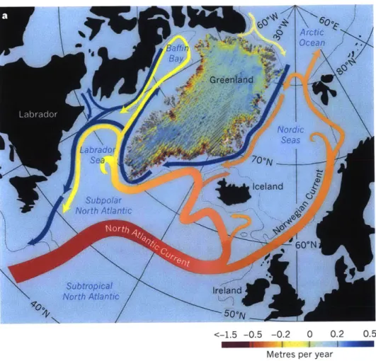
Many outstanding questions regarding the earth's climate lie at the nexus of ocean and cryosphere. The Greenland Ice Sheet is losing 260 Gt/yr of ice and contributing 0.6 mm/yr to global sea level rise (Shepherd et al., 2012). The mass loss is concentrated around the margins of the ice sheet, where glaciers that drain the ice sheet come into contact with the ocean (Fig. 1-1). The largest uncertainties in sea level projections arise from the unknown drivers of ice sheet mass loss in Greenland and Antarctica (IPCC 2013).

For an ice sheet in steady state, snow accumulation over the interior balances ice loss at the margins, through surface melting at the ice-atmosphere boundary and ice discharge at the ice-ocean boundary. The ice discharge can be further subdivided into submarine melting and iceberg calving. For most glaciers around Greenland, the majority of ice is discharged via icebergs (Enderlin and Howat, 2013), in contrast to Antarctica where submarine melting is the dominant mode of ice discharge. Despite its relatively small role in the overall balance mass of the Greenland Ice Sheet, submarine melting has been implicated as a trigger for the recent mass loss.

Approximately one half of the recent mass loss from Greenland is attributed to increased surface melting (van den Broeke et al., 2009), a well understood process: warmer air temperatures have led to more surface melting. The other half of the mass loss comes from changes in ice discharge

- glaciers that drain the ice sheet have accelerated and retreated - but this dynamic component of mass loss is more complicated and poorly understood. The synchronous acceleration of many outlet glaciers originated at their marine termini (Nick et al., 2009; Vieli and Nick, 2011; Howat et al.,

2007) and coincided with warming ocean temperatures around Greenland (Holland et al., 2008a; 11

3ay Greenland SIceland Ireland 60 N b 50'N <-1.5 -0.5 -0.2 0 0.2 0.5

-

r

m

Metres per year

Figure 1-1: Schematic of ocean currents around Greenland from Straneo and Heimbach (2013), with ice sheet surface elevation change from Pritchard et al. (2009), showing mass loss concentrated around the ice sheet's margins. Ice change measurements cover the period of 2003-2007. Currents carrying warm Atlantic-origin water are shown in red

/orange /yellow,

VAge et al., 2011). While there are several possible mechanisms at play, a leading hypothesis is that increased submarine melting at the glaciers' termini triggered a dynamic ice acceleration (Murray et al., 2010; Joughin et al., 2012; Straneo and Heimbach, 2013). Thus, changes in the subpolar North Atlantic and in the Atlantic-origin water that circulates around Greenland (Fig. 1-1) might play a role in driving ice sheet mass loss.

In the other direction, changes in the ice sheet also impact the ocean. The Greenland Ice Sheet is a growing source of freshwater to the polar ocean (Bamber et al., 2012) that could potentially alter coastal currents and eventually the meridional overturning circulation (Weijer et al., 2012; Lenaerts et al., 2015). In addition to providing buoyancy forcing and a net freshening, the input of meltwater at depth drives upwelling of heat and nutrients around the margins of the ice sheet

12

______________1

60

0 C p

(Jenkins, 1999; Cottier et al., 2010; Beaird et al., 2015). The fjords of Greenland are estuaries where glacial freshwater is mixed and exported they form a conduit between the ice sheet and the large-scale ocean. Any change in the ice sheet or ocean that is felt by the other must be communicated through fjord processes.

1.2

Unknown dynamics in glacial fjords

Understanding the coupled evolution of the ocean and ice sheet involves many oceanic scales, from the gyre-scale circulation at 0(1000 kin) down to turbulent fluxes at ice-ocean boundary layer, 0(1

in). While the large-scale ocean circulation around Greenland has been studied for many years, the glacial fjords - where ocean and glaciers directly interact - have been largely overlooked until the past decade.

To set the scene, most of Greenland's marine glaciers terminate in fjords with a vertical calving front, often 100 to 1000 m deep (Fig. 1-2). The major outlet glaciers flow into the ocean at ~10 km/yr (Moon et al., 2012), discharging a volume flux of iceberg and submarine meltwater on the order of 1000 m3

/s.

glacier, rendering the near-glacier waters inaccessible by boat.

plume submarine-meltwater ambient ocean water runoff metponds

front ice ford

600m melange fir

subglacial

I

discharge grounding

(runoff) line

00km

Figure 1-2: Schematic of a typical tidewater glacier/fjord system in Greenland. Inset magnifies the region near the grounding line, where a buoyant plume fed by runoff and submarine meltwater entrains ambient ocean water. Schematic adapted from Straneo et al. (2013).

13

Submarine meltwater is only one source of liquid freshwater to glacial fjords; surface melt also drains through a systems of moulins and channels to the base of the glacier and enters the fjord as subglacial discharge/runoff (Fig. 1-2; Chu, 2014). Thus, the glacier provides two sources of liquid freshwater that form turbulent buoyant plumes at the ocean/ice interface (Jenkins, 2011). The plumes upwell and then, depending on their entrainment rate, either reach the surface or outflow subsurface (e.g. Salcedo-Castro et al., 2011; Sciascia et al., 2013; Stevens et al., 2015). These glacial plumes enter fjords that are typically deep, strongly stratified and composed of the two water masses from the shelf: warm, salty Atlantic-origin water at depth and cooler, fresher Polar-water at the surface (Straneo et al., 2012).

It is warming in this Atlantic-origin water that is believed to have triggered an acceleration of outlet glaciers in the past decade (Holland et al., 2008a; Murray et al., 2010; Straneo and Heimbach,

2013). However, this hypothesis is difficult to test because there are no direct measurements of

submarine melting and only a limited understanding of the fjord circulation or variability. The drivers of heat transport and meltwater export are largely unknown.

The majority of recent work on Greenland's glacial fjords is based on brief summer surveys or modeling. On the modeling side, studies have focused on the upwelling plumes and near-glacier circulation (0(100 m) of the terminus) where there are almost no observations. Modeling studies that explore the controls on submarine melting all show that the melt rate increases with subglacial discharge and with ambient ocean temperature (e.g. Jenkins, 2011; Xu et al., 2012; Sciascia et al.,

2013). These modeling results, however, are sensitive to their parameterizations of turbulent fluxes,

which are tuned to match plume theory. Furthermore, even if these model-derived relationships between ocean temperature, subglacial discharge, and submarine melting are correct, all three of these pieces are poorly constrained by observations.

In the first of these three pieces, the ocean temperature and its variability near glaciers is not well measured. Most studies are based on synoptic shipboards surveys - icebergs pose major obstacles to moorings - and are primarily focused on summer conditions (e.g. Holland et al., 2008a; Rignot et al., 2010; Straneo et al., 2011; Mortensen et al., 2011; Chauch6 et al., 2014). These studies have provided novel insights into the water masses, stratification, and the spread of glacially modified water (often subsurface) (e.g. Johnson et al., 2011; Straneo et al., 2011; Inall et al., 2014). However, given the limited temporal resolution of these fjord surveys and few velocity measurements, little is known about the temperature variability or modes of fjord circulation.

The other two pieces, the subglacial discharge and the submarine melt rate - the direct link 14

between ocean and ice - are also poorly constrained. Neither has been directly measured at the terminus of a tidewater glacier. Subglacial discharge is typically estimated with regional climate models (e.g. Mernild and Liston, 2012; Andersen et al., 2010; Van As et al., 2014). A growing number of studies attempt to infer submarine melting from measurements of ocean heat transport. However, these have been based on brief synoptic measurements, and the prevalent equations of this method are oversimplified, with many implicit and untested assumptions. The complete glacial fjord budgets - of heat, salt and mass - that underlie such methods have never been explored.

Furthermore, modeling studies have focused on the glacier's buoyancy driven circulation, both in the near-glacier region and at the fjord-scale (Xu et al., 2013; Sciascia et al., 2013; Kimura et al., 2014; Carroll et al., 2015). According to the conventional paradigm for Greenland's fjords as a buoyancy-driven regime, the freshwater inputs from glaciers control renewal of water and heat into the fjord, allowing for positive feedbacks between melting and heat transport. There are, however, many other potential drivers of fjord circulation, including tides, local wind forcing, and shelf forcing, that could play an important role in transporting heat and exporting meltwater. Answering questions about the ocean's impact on the glaciers or the glacier's impact on the ocean requires resolving the dynamics of Greenland's glacial fjords.

1.3

Glacial fjords: outliers in the estuarine world

Glacial fjords are fundamentally estuaries. The extensive estuarine and fjord literature, however, does not adequately account for these rogue estuaries. While typical estuaries and fjords have freshwater input at the surface, freshwater from a glacier often enters hundreds of meters below the surface. While typical fjords have a shallow sill and only one oceanic water mass inside the fjord, Greenland's glacial fjord are usually deep and strongly stratified with multiple water masses from the shelf. While friction plays a dominant role in most estuaries, often balancing an along-estuary pressure gradient, friction should be relatively weak in the deep fjords of Greenland. Lastly, instead of being spread throughout the estuary or concentrated at topographic features, the vast majority of mixing in glacial fjords occurs where convective plumes emanate from the glacier. For these and other reasons, the existing estuarine paradigms are largely inapplicable to Greenland's glacial fjords.

along-shore along-fjord wind

shelf winds 0 A calving

submarine

Pa meltwater

>mass

runoff shelf fjord

Figure 1-3: Schematic of glacier, fjord and shelf, including some potential drivers of circulations: shelf winds and shelf density variability: local along-fjord winds; and freshwater from the glacier

(submarine melting and runoff).

1.4

Driving questions of this thesis

This thesis aims to answer fundamental questions about the dynamics of Greenland's glacial fjords. Observations, theory, and numerical modeling are used to investigate the drivers of fjord circulation, heat transport and freshwater export near outlet glaciers. The driving questions of this thesis, which

are also illustrated in Fig. 1-3, are as follows:

Chapter 2:

" What are the dominant drivers of circulation in east Greenland's glacial fjords? " What drives temperature variability near glaciers?

Chapter 3:

" What are the dominant balances in the heat, salt and mass budgets for a glacial fjord? " How are heat, salt and meltwater transported through the fjord?

" What are the magnitudes and seasonality of the freshwater fluxes (submarine melting and runoff) into glacial fjords?

Chapter 4:

" How does shelf density variability drive fjord flows in fjords around Greenland? " What is the relative importance of shelf forcing versus local wind forcing?

Thesis outline

In Chapter 2, the drivers of fjord circulation and variability are explored in two major fjords of east Greenland. Moored records of velocity and water properties show rapid exchange between the shelf and fjords that is driven by shelf density fluctuations (which are primarily associated with

along-shore winds). These synoptic shelf-driven flows allow the fjords to track shelf variability on short timescales and result in large temperature fluctuations in the upper fjord, near the glacier. Contrary to the conventional paradigm for glacial fjords, these flows mask any glacier-driven circu-lation during the non-summer months. The submarine melt-rate is dependent on the near-glacier temperature and velocity, so these shelf-forced dynamics are important for accurate modeling and

prediction of submarine melting.

In Chapter 3, the heat, salt and volume budgets for glacial fjords are explored in order to understand the dominant balances and modes of transport, and also to quantify the heretofore unknown freshwater fluxes and their seasonality. Building on estuarine studies of salt budgets, we present an alternative framework for decomposing fjord budgets and new equations for inferring meltwater fluxes. These methods are then applied to moored records from Sermilik Fjord, near the terminus of Helheim Glacier, to evaluate the dominant balances in the fjord budgets and to estimate freshwater fluxes. Seasonally, we find two different regimes of heat, salt and meltwater transport. Our results highlight many important components of fjord budgets, particularly the storage and barotropic terms, that have been neglected in previous estimates of submarine melting. Additionally, these provide the first timeseries of subglacial discharge and submarine meltwater fluxes into a a glacial fjord.

In Chapter 4, the dynamics of shelf-forced flows in fjords are investigated with numerical simu-lations and theory to explore the nature of shelf-driven circulation and how it varies across different fjords. Building on the observations Sermilik Fjord, we use ROMS numerical simulations and two analytical models to study the dynamics of shelf-driven flows and their competition with local forc-ing within a fjord. We investigate the relative importance of the shelf forcforc-ing in drivforc-ing fjord/shelf exchange across a wide parameter space of fjord geometries and stratifications.

Overall, this thesis investigates the drivers of fjord circulation, heat transport, and meltwater export in Greenland's glacial fjords, aiming to make a step towards understanding ocean-glacier interactions and towards accurate modeling of coupled ice sheet/ocean evolution in a changing climate.

Chapter 2

Externally-forced fluctuations in ocean

temperature at Greenland glaciers in

non-summer months

This chapter was originally published as: Jackson, R. H., Straneo, F. & Sutherland, D. A.: Exter-nally forced fluctuations in ocean temperature at Greenland glaciers in non-summer months. Nature

Geoscience, 7, 503-508 (2014). Used with permission as granted in the original copyright agreement.

2.1

Abstract

Enhanced submarine melting of outlet glaciers has been identified as a plausible trigger for part of the Greenland Ice Sheet's accelerated mass loss (Thomas, 2004; Holland et al., 2008a; Vieli and Nick, 2011), which currently accounts for a quarter of global sea level rise (Shepherd et al., 2012). However, our understanding of what controls the submarine melt rate is limited and largely informed

by brief summer surveys in the fjords where glaciers terminate. Here, using continuous water property and velocity records from September through May in two large fjords - into which Helheim and Kangerdlugssuaq Glaciers drain - we show that water properties, including heat content, vary significantly over synoptic timescales 3 to 10 days. This variability results from frequent, shelf-forced pulses that drive rapid exchange with the shelf and mask any signal of a glacial freshwater-driven circulation. Our results suggest that, during non-summer months, the melt rate varies substantially and is dependent on externally-forced ocean flows that rapidly translate changes on the shelf towards

the glaciers' margins.

2.2

Introduction

The submarine melt rate depends on near-glacier ocean temperature and circulation (e.g. Jenkins et al., 2010). Recent studies assume that both these things are governed by the glacier's freshwater inputs (Motyka et al., 2003; Rignot et al., 2010; Jenkins, 2011; Xu et al., 2012; Sciascia et al., 2013), and that other drivers, such as tides, air-sea fluxes and shelf-driven exchange, can be neglected. In this prevailing framework, submarine meltwater and subglacial discharge (surface meltwater draining at the glacier's base) form buoyant plumes, entrain ambient water and drive an overturning circulation that transports shelf waters towards the glacier. Under this assumption, enhanced subglacial discharge increases ocean heat transport, submarine melting, and the renewal of near-glacier waters (Jenkins, 2011; Xu et al., 2012; Sciascia et al., 2013).

However, the extent to which the glacier-driven circulation influences the renewal of warm water in the fjords is unclear. Limited velocity data indicates that shelf variability may play an important role in driving fjord flows (Rignot et al., 2010; Straneo et al., 2010), though conclusive evidence is absent. Furthermore, most observational studies rely on brief, summer surveys (Holland et al., 2008a; Rignot et al., 2010; Christoffersen et al., 2011; Straneo et al., 2011; Johnson et al., 2011; Xu et al., 2013; Inall et al., 2014) that offer limited insight into drivers of summer variability and no information about non-summer months.

2.3

Setting

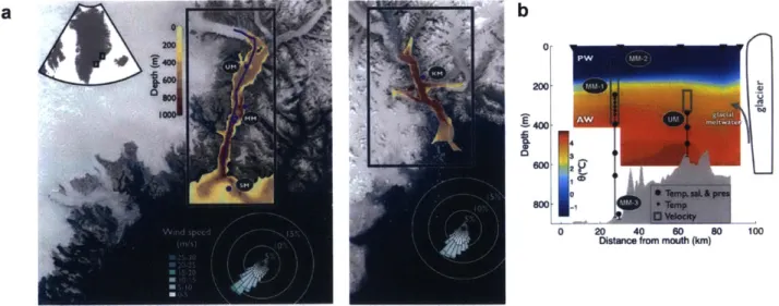
Here, we present new insight into fjord dynamics from moored records in Sermilik and Kangerd-lugssuaq Fjords (Fig. 2-1a), where Helheim and KangerdKangerd-lugssuaq Glaciers deposit freshwater as submarine meltwater, subglacial discharge, surface runoff, and icebergs. These are the fifth and third largest outlets of the Greenland Ice Sheet, respectively, in terms of total ice discharge (En-derlin et al., 2014). The vertical calving fronts of both glaciers ground ~600 m below sea level at the head of their respective fjords (Straneo et al., 2012). The fjords, which are ~70/100 km long and ~7 km wide, connect the glaciers to the continental shelf. The predominant water masses of Greenland's southeast shelf form a two-layer structure within Sermilik Fjord: cold, fresh Polar water (PW) overlies warm, salty Atlantic-origin water (AW), with some modification due to glacial inputs (Fig. 2-1; Sutherland and Pickart, 2008; Straneo et al., 2010, 2011). A similar water mass structure

is found in Kangerdlugssuaq, with additional dense Atlantic water originating in the Nordic Seas (Christoffersen et al., 2012). In both Sermilik and Kangerdlugssuq fjords, the shallowest sills (at

530 and 550 m, respectively) are well below the AW/PW interface (Schjoth et al., 2012: Sutherland

et al., 2013; Inall et al., 2014), allowing for relatively unimpeded exchange between the fjord and shelf (bathymetry shown in Fig. 2-1a & b). The shelf region of southeast Greenland outside both fjords is characterized by frequent, strong, along-shore winds (Harden et al., 2011) and fast ocean currents (Sutherland and Pickart, 2008).

Winds and glacial freshwater discharge - two potential drivers of fjord circulation - exhibit a strong seasonality in this region. From September through May, shelf winds are strong along Greenland's southeast coast (Harden et al., 2011), and subglacial discharge is negligible as air tem-peratures drop below freezing (Mernild et al., 2010; Andersen et al., 2010). During summer, winds weaken, and subglacial discharge increases, becoming a larger freshwater source than submarine melt (Mernild et al., 2010; Andersen et al., 2010). This seasonality likely modulates the glacier-driven circulation and submarine melt rate; one modeling study estimated the summer melt rate at Helheim Glacier to be twice the non-summer rate due to variations in subglacial discharge (Sciascia et al., 2013). According to this scaling, nevertheless, 60% of the annual submarine melt would occur in non-summer months, an important but unstudied period.

a

b

020

00-.600 .. 0

8001

J2-0 Temp. sal, & pres

S800 Temp

t Velocity

0 20 14C 60 80 100

Distance from mouth (km)

Figure 2-1: a. Satellite images of Sermilik and Kangerdlugssuaq Fjords with bathymetry overlaid. Circles indicate mooring locations and line shows path of along-fjord Sermilik profile in (b). Wind roses of speed and direction on the shelf are from ERA-Interim Reanalysis from 2009-2013. b. Along-fjord potential temperature from 2010 winter survey of Sermilik (Straneo et al., 2011) with schematic of Sermilik moorings (shelf mooring, SM, not shown), instruments and water masses. AW

= Atlantic-origin water; PW = Polar-origin water.

2.4

Data: moorings and wind

Extensive oceanic water property and velocity records were collected during the non-summer months in 2011-2012 from Sermilik Fjord and the adjacent shelf (Fig. 2-2a-d) and in 2009-2010 from Kangerdlugssuaq Fjord (excluding velocity, Fig. 2-2e).

Ii

I~

IL

;jt

1/

I

I

Oct/11 Nov Dec

A

~f

j\J

\

Jan/12 Feb Mar

1~r;

KM

Oct/09 Feb Mar

Figure 2-2: a. Along-fjord velocity in Sermilik at mid-fjord mooring (MM1); b. Along-fjord veloicty at upper-fjord mooring, UM. In both positive indicates up-fjord flow, towards the glacier. c. Potential temperature in Sermilik at mid-fjord, MM1-3. d. Potential temperature at upper-fjord,

UM. Contours of -o = [27.0, 27.5] kg'/m3 overlaid. e. Potential temperature in Kangerdlugssuaq at

mid-fjord (KM1-3) for same nine months but different years (2009-2010). All records are low-pass filtered with a 4th order 26-hr Butterworth filter. Black line in a-d marks an up-fjord flow in the lower layer that is highlighted in Fig. 2-8.

22

a

Ii

0.8

d

e

Nov Dec Jan/10

I

r

n "

V

In the Sermilik region, we deployed five moorings (SM, MM 1-3 and UM; locations in Fig. 2-1) to capture velocity in the fjord and water properties in the fjord and on the shelf. An upward-facing 75 kHz Acoustic Doppler Current Profiler (ADCP) on MM-1 measured velocity in 10 m bins between

388 m and the surface from August, 2011 through June, 2012. The upper three bins (centered at 28, 18 and 8 m) were discarded due to side-lobe contamination. An upward-facing 300 kHz ADCP

on UM measured velocity in 8 m bins between 313 and 233 m from August, 2011 to September, 2012. Both instruments measured 10-minute averaged velocity every hour. Gaps in the records

-often from instrument contamination (e.g. icebergs) or low-backscatter - were filled by removing a tidal fit, interpolating linearly, and adding back the tidal component. The along-fjord velocity was determined by rotating the velocity field into its principal axes and extracting the component along the major axis, which falls parallel to local bathymetry at both locations (320 and 350 from north at MM-1 and UM, respectively). The across-fjord velocities along the minor axis were smaller (with variance ~90% smaller than along-fjord variance) and are not discussed here.

Concurrently, nine conductivity-temperature-pressure sensors (Seabird SBE 37SMs and RBR

XR-420s at 291 m on SM, 125, 246, 396, 542, 657 and 851 m on MM 1-3 and 323, 406 and 510 m

on UM) and five temperature sensors (Onset Tidbit v2 at 266, 286, 306, 326, and 346 m on MM

1-3) recorded water properties. All temperature records from the mid-fjord moorings, MM 1-3, were

combined to make the depth versus time contour plots in Fig 2-2d, thereby neglecting horizontal variability between the nearby moorings. This approximation is supported by the synoptic surveys of the fjord and moored records, which show that the horizontal spatial variability within several kilometers is small compared to the variability in depth and time. Hydrographic surveys of the fjord were conducted upon mooring deployment and recovery and used to calibrate the moored instruments.

In Kangerdlugssuaq Fjord, we deployed three mid-fjord moorings (KM1-3) from August, 2009 to September, 2010 (location in Fig. 2-1). Two temperature-conductivity-depth sensors (RBR XR-420s) were deployed at 166 m and 225 m on KM1 and KM2, respectively. KM3 was equipped with a depth recorder (RBR DR-1050) at 223 m and seven temperature sensors (Onset Tidbit v2) at 223

243, 253, 263, 273, 283 and 303 m depths.

The ERA-Interim reanalysis, deemed successful at capturing winds on the shelf of southeast Greenland (Harden et al., 2011), is used to assess the shelf wind field. Outside of Sermilik and Kangerdlugssuaq Fjords, the velocity component along the principle axis (230' and 2100 from north, respectively) at a point 45 km offshore of each fjord's mouth was extracted for an along-shore wind

time-series (locations and wind roses in Fig.2-la; time-series in Fig. 2-4a). By this convention, downwelling-favorable winds from the northeast are positive.

2.5

Results

In Sermilik Fjord, the records indicate that AW and PW are always present, but their properties and thicknesses vary over timescales of hours to months (Fig. 2-2c & d). The upper water column near the AW/PW interface exhibits the largest variability, a result of both seasonal trends (Straneo et al., 2010) - e.g. PW deepening and cooling in the winter - and higher frequency fluctuations in the interface's depth, often exceeding 50 m over several days (Fig. 2-2c & d). Within the AW layer, temperature ranges from 2'C to 5.2'C and exhibits transient fluctuations (typically 0.3-0.7'C) that last several days, and more sustained shifts, such as an abrupt cooling in late March. Significant variability even exists at 851 m, well below sill depth.

The fjord's persistent stratification and occasional increases in heat content preclude internal mixing (which would reduce stratification and redistribute heat) or surface fluxes (which would reduce stratification and cool) from being the primary drivers of these changes. Instead, as will be shown here, we attribute the variability to rapid exchange with the shelf, driven by energetic, sheared flows in the along-fjord direction (Fig. 2-2a & b).

2.5.1 Description of velocity field

These pulses last several days and frequently exceed 50 cm/s in the upper layer, with mid-fjord root mean squared (RMS) velocities at all depths between 10 and 20 cm/s - much larger than the -2.5 cm/s root-mean square tidal component (Fig. 2-2a). The velocity typically reverses direction at the AW/PW interface (i.e. pycnocline) and is faster in the upper layer.

An EOF analysis of the mid-fjord velocity shows that the velocity structure is consistent with the first baroclinic dynamical mode calculated from the fjord stratification. An EOF analysis was performed both in a standard depth coordinate and in a rescaled depth coordinate based on the density field. In this latter transformed space, zero corresponds to the top of the velocity record, one to the bottom of the record, and 0.5 to the depth of the o = 27 kg/m3 isopycnal (after detrending with a 30-day 4th order Butterworth filter and adding back the mean), which is a proxy for the pycnocline or AW/PW interface. This rescaled depth variable was used to account for the variability in layer thicknesses. Similar results were found in both EOF analyses, with almost

identical mode structures, although the first EOF in transformed space captured slightly more of the record variability (67% versus 62%). A section of the raw velocity record and the velocity reconstructed from the first EOF are shown in Fig. 2-3a, with the isopycnal used for scaling. This two-layer flow has peak variability at 4-10 day periods, i.e. synoptic timescales, as shown in the power spectrum of the first EOF's principle component (Fig. 2-3c).

We find that the first EOF mode structure closely resembles the first baroclinic mode based on the fjord stratification (Fig. 2-3b). Winter profiles from a survey of Sermilik Fjord in March, 2010 (Straneo et al., 2011) were used in conjunction with the moored water properties to construct a mean stratification profile and then compute the first baroclinic mode structure.

Upper-fjord velocities at UM (Fig. 2-2b) are reduced but well correlated with mid-fjord flow. RMS velocities in the upper fjord are approximately 5 cm/s, compared to a tidal component of 1 cm/s. If the AW/PW interface movements are approximately coherent throughout the fjord over the pulse timescale, we would expect the velocity to decay linearly towards the glacier in a rectangular fjord. Thus, we expect the upper-fjord speeds to be approximately 36% of those mid-fjord, based on the distance between UM and the head of the fjord (20 km) and between MM and UM (37 km), which is consistent with our observations. The velocities at UM and MM in the 320-290 m depth range are significantly correlated for every velocity bin (correlation coefficients all greater than >

0.45).

2.5.2

Mid-fjord volume flux

The velocity pulses drive large volume transports and significant exchange with the shelf over short timescales. To calculate a time-series of volume fluxes in Sermilik (Fig. 2-4c), we assume that the mid-fjord velocity field is uniform across the width of the fjord at the mooring location. This is based on previous studies of lowered ADCP and CTD sections (Straneo et al., 2011; Sutherland and Straneo, 2012) that show small lateral shear across the fjord. Thus, we calculate volume flux in the

upper layer as:

Q

where: h equals 10 m, the depth range of each bin; W equals 7 km, the approximate width the fjord at the mooring location; n is the last bin above the AW/PW interface. This interface was chosen to be the 27 kg/m3 potential density contour from the 30-day high-pass filtered density field. The

a. 100 200~ -W T 300 _Raw 'a ' q

~

24-Oct 13-Nov 03-Dec 23-Dec 12-Jan 01-Feb

b. 0 100 200 0 300 400--1st EOF = 67% variance .2nd EOF = 20% 3rd EOF = 7% 1 st baroclinic mode -.3 -0.2 -0.1 0 0.1 0.2 0.3 C. 4-10 days 10 10 10 10 10 10-3 10-2 10 Freq (1/hr)

Figure 2-3: a. Subsection of velocity record: raw (upper), first EOF multiplied by its principal component (middle), and residual after removing first EOF (lower). Density contour used for rescaling depth overlaid. b. Vertical structure of the first three EOFs of the velocity record and the first baroclinic mode as calculated from the density structure. c. Power density spectrum of the principle component of first mode EOF as a function of period, with peak at 4-10 day periods marked.

velocity record excludes the top 33 m of the water column, so four methods are used to extend the velocity profile to the surface and put an error estimate on the volume flux (Fig. 2-4c). The surface velocities were filled in with: 1) a constant value equal to the top bin, 2) an extension of the mean shear observed in the depth range of 33 to 73 m, 3) a linear shear such that the velocity goes to zero at the surface, and 4) no velocity. The lower layer volume flux was not directly calculated because the velocity record ends at 400 m; however, we can infer it to be of approximately equal magnitude and opposite direction as the upper layer flux based on our knowledge of the density profile and presumed conservation of fjord volume.

The average volume exchanged in each layer over the 16 strongest pulses is 8.5+0.8 x1010 m3 _ equivalent to -50% of the average upper layer volume in the entire fjord or ~25% of the lower layer. This was determined by time-integrating the upper layer volume flux over a pulse to determine the total volume exchanged and then comparing it to each layer's total volume in the fjord based on a mean interface depth of 180 m. Average volume exchanged during a pulse is compared to the total volume of each layer, though the fraction of water exchanged would be 35% higher if compared to the volume of each layer upstream of the mooring, i.e. between the mooring and the glacier.

2.5.3 Fjord flows driven by shelf variability

We attribute these large volume fluxes to forcing from the shelf, through a pumping mechanism that is sometimes called the intermediary circulation. Shelf winds, waves, or other phenomena drive density fluctuations and sea surface height anomalies at the fjord's mouth that can propagate up-fjord and drive flow within the up-fjord (e.g. Stigebrandt, 1981; Klinck et al., 1981). This mechanism has been found to force more fjord/shelf exchange than tidal or estuarine flows in some Scandinavian fjords (Stigebrandt, 1990; Arneborg, 2004). A previous summer study of Sermilik hypothesized that shelf forcing may be important for flushing the fjord (Straneo et al., 2010); however, until now, no direct evidence of this mechanism or its associated variability existed in Greenland's fjords.

Examination of the velocity pulses in our data reveals a structure consistent with strong shelf forcing. Composites of the mid-fjord velocity, mid-fjord density, shelf density and shelf pressure (Fig. 2-5) were created by averaging these fields over the 16 strongest velocity pulses. These events were defined by an up-fjord volume flux (26-hr low-pass filtered) in the upper layer exceeding 3.7x 105

m3 s- 1and aligned by the time of peak volume flux. The pulses are identified by grey shading in

Fig.2-4a. The composites illustrates the basic features of these pulses: the PW layer thickens, associated with depressed isopycnals, as a strong up-fjord flow develops above the interface and a

1 -1 EI0.5- 8- 6-2 -WW~ Al) 1 Q 0 -2 -4 d « V

(~JA

Oct Nov Dec Jan/12 Feb Mar Apr May

Figure 2-4: a. Along-shore wind stress on the shelf outside Serinilik; positive winds are to the southwest, i.e. downwelling-favorable. b. Potential density from shelf mooring (SM) at -291 m depth. c. Volume flux in upper layer at mid-fjord mooring (MM), assuming uniform across-fjord velocity; positive indicates flow towards the glacier. d. Variability (as percent deviation from the mean) in submarine melt rate based on a linear or quadratic scaling law between melt rate and average water column temperature (Appendix 2.A). Shading in all panels over the 16 strongest pulses, which were used to for the composites in Fig. 2-5.

weaker out-flow below. Velocity in each layer then reverses as the density field rebounds. These pulses originate on the shelf with a negative density anomaly and positive bottom pressure anomaly (indicating a positive sea-surface height anomaly), and the density anomaly then propagates up-fjord at speeds approximately matching the first baroclinic mode gravity wave phase speed.

a

Hours from peak volume flux

Figure 2-5: Composites of various records over 16 strongest velocity pulses (defined by up-fjord volume flux in upper layer exceeding 3.7xI05 M3 s-1; see Fig. 2-4a). a. Composites of potential

density anomaly (30-day low-pass signal removed) and bottom pressure anomaly from shelf mooring

(SM) at ~291 in depth. b. Composite of mid-fjord velocity (MM) with contour of - = 27.0 kg/m3

from composite of mid-fjord potential density (30-day low-pass signal removed, mean added back). Positive velocities indicate flow up-fjord. towards the glacier.

The structure of velocity pulses shown in the composite (Fig. 2-5) is confirmed by a high coher-ence amplitude between fjord velocity, fjord density and fjord bottom pressure on synoptic timescales of 2-10 day periods (Fig. 2-6a) with 95% confidence. The coherence phase between these records confirms that negative density anomalies coincide with, and positive pressure anomaly precede, in-flow in the upper layer. The records onl the shelf are also highly coherent with the fjord records

29

in the same synoptic timeband (Fig. 2-6b), with phases confirming the origin of these signals on the shelf. The shelf mooring is dynamically up-stream of the fjord in the East Greenland Coastal Current and thus we do not expect its signal to be significantly influenced by the fjord.

2 days 10 days

a

b

C

~

midfjord vel & midfjord pres midfjord vel & midfjord dens

- upfjord vel & upfjord dens

shelf wind & shelf dens

-- shelf wind & shelf pres shelf wind & mid-fjord vel

102

Figure 2-6: Coherence amplitude as a function of period (in hours) for many pairs of records from moorings and wind field (see legends): a. at the same fjord moorings, b. at different fjord

/shelf

All fjord velocity pulses are associated with shelf density fluctuations, and most are also preceded by along-shore, downwelling-favorable winds on the shelf that are typical of this region (Fig. 2-4).

These winds depress isopycnals and raise the sea surface towards the coastline, resulting in the shelf/fjord set-up described above. The link between shelf wind and shelf fluctuations - which

30

--

I

~0

-shelf dens & midfjord dens

shelf dens & upfjord dens

- shelf dens & midfjord vel shelf dens & upfjord vel

midfjord dens & upfjord dens midfjord vel & upfjord vel

0

-

create shelf/fjord gradients - can be seen in the high coherence between along-shore wind, shelf pressure and shelf density at 2-10 day periods (Fig. 2-6c). We speculate that other phenomena such as coastally trapped waves and eddies can generate fjord/shelf pressure gradients, resulting in occasional pulses without associated winds (Fig. 2-4).

Preceding most in-flowing pulses in the upper layer, the bottom-mounted pressure (after de-tiding, smoothing with a 26-hr Butterworth filter and removing a 30-day trend) at SM and MM both show an average positive pressure anomaly of 0.1 db (e.g. Fig. 2-5). This bottom pressure can be a function of density changes as well as changes in sea surface height:

/0

PWz = pogrq +

jz

where P(z) is the pressure at depth z, q is the sea surface height, p is the density, and Pa is the atmospheric pressure. At MM, we can estimate the contribution to bottom pressure from density variability with the CTD records (Fig. 2-2) and find that it opposes the average pressure anomaly

by -5 cm, and thus we estimate the average change in surface height to be ~15 cm. This sea surface set-up on the shelf and in the fjord is consistent with on-shore transport from downwelling-favorable winds.

A cross-correlation analysis of the density records and shelf wind (Table 2.1) illustrates the shelf

forcing and propagation of signals between moorings. Negative density anomalies are associated with downwelling-favorable (positive) winds, hence the negative correlation between wind and density. Density at all three locations have cross-correlation coefficient greater than 0.7 with each other. Density at mid-fjord lags density on the shelf by 14 hours, while upper-fjord density lags mid-fjord

by 17 hours. For comparison, we expect these signals to propagate at the first baroclinic mode

phase speed, which we estimate to be 1 m/s based on the density stratification. The shelf/mid-fjord and mid-fjord/upper-fjord distances are 32 km and 37 km, respectively. These result in expected propagation times of 10 and 11 hours, respectively. Thus, the propagation speeds that we observed are similar, though somewhat slower (which could be explained by the presence of icebergs in the

fjord (MacAyeal et al., 2012)).

2.5.4 Changes in heat content

Regarding the glacier, these pulses significantly alter the fjord's heat content via changes in layer thickness and property shifts within layers. All pulses have, at least, a transient response from

__ correlation coeff.

Jlag

/

/

/

Table 2.1: Peak correlation coefficient and lag at peak correlation between various records: shelf wind, shelf density at SM, mid-fjord density at MM and upper-fjord density at UM. T is wind; a is density. All correlations are statistically significant at 99% confidence. Positive lags indicates first record leads second record.

the first effect, e.g. up-fjord flow in the PW layer thickens that layer, increasing the volume of PW relative to AW and decreasing the average water-column temperature. The PW/AW interface moves ~50 m vertically during each velocity pulse, resulting in large heat content fluctuations. The average water column temperature above 630 m (the glacier's grounding line depth), shown in Fig. 2-7, consequently drops by 0.6'C on average with strong in-flow in the upper PW layer. The upper layer volume flux and average water column temperature are highly coherent (>95% confidence) at 2-11 day periods.

All pulses drive transient changes in layer thickness and are associated with heaving isopycnals

on the shelf. Only some pulses, however, advect new properties into the fjord, which, we argue, reflect changes in water properties on the shelf. Shifts in AW temperature often coincide with lower layer in-flow during energetic pulses. For example, Fig. 2-8 highlights one such event where the temperature at both MM and UM increases in the thermocline and in AW layer, coinciding with up-fjord velocity in the AW layer (black line in Fig. 2-2).

To compare AW layer properties at mid- and upper-fjord, the potential temperature records from MM and UM were each interpolated onto a 10-m vertical grid and averaged between 350 m and 530 m. A cross-correlation of the average AW temperature between UM and MM shows that the upper-fjord lags mid-upper-fjord by 26 hours (correlation coefficient = 0.55), corresponding to a propagation speed of 0.4 m/s. This is significantly slower than the density signal, which appears to propagate along the pycnocline as a first baroclinic mode wave. This suggests that the temperature anomalies within the AW layer, which typically do not have a strong density signal, are being advected by the flow at approximately 0.4 m/s - a speed that compares well to the mean velocity over one direction of a pulse.

Upper layer volume flux

Oct Nov Dec Jan/12 Feb Mar Apr May

Mean mid-fjord temperature above 630m

Oct Nov Dec Jan/12 Feb Mar Apr May

Figure 2-7: a. Upper layer volume flux (same as Fig. 2-4c) b. Average water column potential temperature above 630 m (i.e. the depth range of glacier's face) from mid-fjord records. Grey bars highlight the 16 strongest up-fjord pulses.

33

a

b

a

b

Figure 2-8: Potential temperature profile during 4-day periods proceeding and following a strong up-fjord flow (indicated with black lines in Fig. 2-2) in the AW layer at mid-fjord mooring (a) and upper-fjord mooring (d). Circles show average temperature at instrument during each period; shading indicates 95% range of all measurements over this period.

2.5.5 Shelf forcing in Kangerdlugssuaq Fjord

The mid-fjord water properties from Kangerdlugssuaq Fjord exhibit similar variability to Sermilik: large-amplitude fluctuations in the thermocline (Fig. 2-2e) and significant variability at synoptic timuescales. We find a statistically significant peak in coherence between the density records in Kangerdlugssuaq at 3-12 day periods, similar to the results from Serrmilik.

The relationship between shelf wind and fjord properties indicates that shelf-forcing is likely a dominant driver of variability in Kangerdlugssuaq (Fig. 2-9). Without a shelf mooring outside