Earthquake source parameters, seismicity, and tectonics of North Atlantic transform faults

EARTHQUAKE SOURCE PARAMETERS, SEISMICITY, AND TECTONICS OF NORTH ATLANTIC TRANSFORM FAULTS

by

JAMES LOUIS MULLER

B.S., Virginia Polytechnic Institute and State University (1971)

S.M., Massachusetts Institute of Technology (1982)

SUBMITTED TO THE DEPARTMENT OF EARTH AND PLANETARY SCIENCES IN PARTIAL FULFILLMENT OF THE REQUIREMENTS FOR THE DEGREE OF

DOCTOR OF PHILOSOPHY at the

MASSACHUSETTS INSTITUTE OF TECHNOLOGY January, 1983

A

Signature of Author . '--.'% . . .

Department of Earth and Planetary Sciences Certified by . - - . -.- . . . . . . .. .. .. .. . Sean C. .Solomon Thesis Supervisor Accepted by . . .-. . . . ... . .y . , . . . ... Theodore R. Madden Chairman, Department Graduate Committee MASSA4USE fS INSTITUTE OF TECHNOLOGY

MAR 14 19Q3

EARTHQUAKE SOURCE PARAMETERS, SEISMICITY, AND TECTONICS OF NORTH ATLANTIC TRANSFORM FAULTS

by

James Louis Muller

Submitted to the Department of Earth and Planetary Sciences Massachusetts Institute of Technology

on January 24, 1983,

in partial fulfillment of the requirements for the degree of Doctor of Philosophy

ABSTRACT

Earthquakes on oceanic transform faults provide a record of plate motion in space and time. This thesis is a study of the recent history of displacement on six transform faults on the Mid-Atlantic

Ridge, as revealed by the source characteristics of teleseismically recorded earthquakes. We have investigated the seismic history of the Gibbs, Oceanographer, Kane, 15* 20', Vema, and Doldrums transform faults, and we have determined the source parameters of twelve large earthquakes

(Ms 5.1 to 7.0) on these transform faults by constructing synthetic

seismograms to match observed P waveforms from WWSSN long-period vertical

seismograms. The approximate latitudes of the transforms studied are

520N, 350N, 240N, 15020'N, 110N, and 7*N, respectively.

Synthetic seismograms were constructed using the method of Langston and Helmberger (1975). This technique uses the superposition of the direct P wave with the surface reflections pP and sP, with the latter

phases delayed in time to account for the additional travel path. All amplitudes were adjusted to account for the radiation pattern of the earthquake, and amplitudes of the reflected phases were also corrected for reflection at the free surface. The resulting source waveforms were then convolved with an attenuation operator and corrected for geometrical spreading, and the appropriate WWSSN instrument response was applied. We modified this method to include the effects of a layered velocity

structure near the source and of a finite fault, along which either unilateral or bilateral rupture proceeds horizontally. The effect of fault width (vertical dimension) was shown to be significant, though resolution of fault width is poor because of tradeoff with other.source parameters and insufficient understanding of the rupture process.

Synthetic seismograms were constructed using various combinations of fault parameters until waveforms were found which matched those of observed seismograms.

iii

Synthesis of the P waveforms from twelve transform fault earthquakes indicates strike-slip mechanisms on nearly vertical faults oriented along the strike of each transform. SeisTc moments fo5₇the events varied by over a factor of 100, from 9.5 x 10 to 1.3 x 10 dyne-cm. The focal

depths varied between 1 and 6.5 km below the top of oceanic basement.

Unilateral rupture propagation was indicated for the source mechanisms of

six of the earthquakes studied, and was suggested for another, with a

consistency of propagation direction for each transform. The predominant period of the first half cycle of the observed waveforms was generally no more than about 15 sec and varied little among the earthquakes studied,

despite the broad range of moments found. Fault lengths ranged from 6 to

30 km except for one complex event, which required a multiple source with

a total fault length of 60 km. Average displacements for these events ranged from 0.9 to 12 m.

We compared Ms, mb, and MO values of these earthquakes and others on oceanic transform faults. By restricting the earthquake group to the transforms considered in this study, i.e., to one tectonic setting and to

consistent observational procedures, we derive linear relations between

Ms and mb and between Ms and log Mo that faithfully represent our data with little scatter. Using these relations we have estimated the total

seismic moment released by earthquakes on each transform since 1920 and compared each result with the cumulative moment predicted by the

transform length and the local spreading rate. Those transforms which had large earthquakes toward the beginning of historic seismic

observations had an observed moment total greater than predicted, while those with early seismicity more comparable to that of the entire period showed better agreement. The historical record of large earthquakes on these transforms indicates that each transform slips in a jerky manner and along small fault segments rather than in large events involving

rupture along the entire length of the transform. The repeat time for

Ms ~ 6 events on the part of the transform fractured by each event varied

from about 30 to about 350 years. There may be some correlation between

transforms of the times of occurrence of the largest earthquakes.

ACKNOWLEDGEMENTS

This work would not have been possible without the ideas, work, inspiration, and understanding of many people. Foremost of these has been my advisor, Dr. Sean C. Solomon, who provided the original concept and many of the ideas (and financial support) for this work, who insisted on my getting everything right (or as near to right as I could make it) and thus taught me how real work is done, who acted as primary reviewer of this document, and who(se patience probably wore thin enough that he) forced me to accomplish something tangible. I am grateful for all of these things. I would also like to thank Mark Murray, who compiled much of the earthquake data in the seismicity tables in Chapters 3 to 8, thus saving me lots of time and providing a seed crystal for my doing the rest of it. Thanks also go to Wai-Ying Chung, who provided the original

synthetic seismogram program, to Eric Bergman, who provided programming, ideas, inspiration, and the substance of several figures presented here,

to Rob Comer, Dan Davis, J. Lynn Hall, W. Roger Buck IV, Mark Willis, and

Gerardo Suarez who provided necessary inspiration and idea exchange, and to Jan Nattier-Barbaro (Word Wizard), who made it real. Finally, I would

like to thank my wife, Sharon J. Horovitch, Ph.D., who showed me that it can be done, and who provided the support and understanding for me to do likewise.

This research was partially supported by the National Science Foundation, Earth Sciences Section, under NSF Grants EAR 77-09965 and EAR-8115908.

TABLE OF CONTENTS page Abstract . . . . . . . . . . . . . . . . . . . ... . . . ii Acknowledgements . . . .. ... . . . . . . . . . . . . . . . . . iv Table of Contents . . . . . . . . . .. . . . . . . . . .. . . . . v Chapter 1. Introduction . . . . . . . . . . . . . . . . . . . . . 1

General Concept of Transform Faults 1 Geologic Setting of North Atlantic Transform Faults 2 Transform Fault Seismicity 6 Large Earthquakes on North Atlantic Transforms 8 Objectives of this Study 9 Figures 12 Chapter 2. Method of P-Wave Synthesis . . . . . . . . . . 14

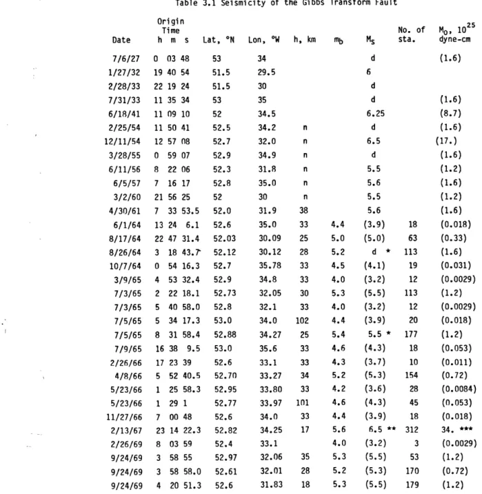
General Technique 14 Modifications 18 The Problem of Finite Width 21 Checks on the Validity of the Method 27 Parameters and Data Needed 30 Resolution of and Ambiguities in the Results 31 Figures 40 Chapter 3. The Seismicity and Tectonics of the Gibbs Transform Fault . . . . .. . . . . . . . . . . . . . .. 54

Seismicity 55

Major Earthquakes 56

Total Seismic Moment 59

North Atlantic Transform Behavior 61

page

Figures 65

Chapter 4. Earthquakes and Tectonics of the Oceanographer

Transform Fault . . . . . . . . . . . . . . . . . . . 68

Seismicity 70

The May 17, 1964 Earthquake 71

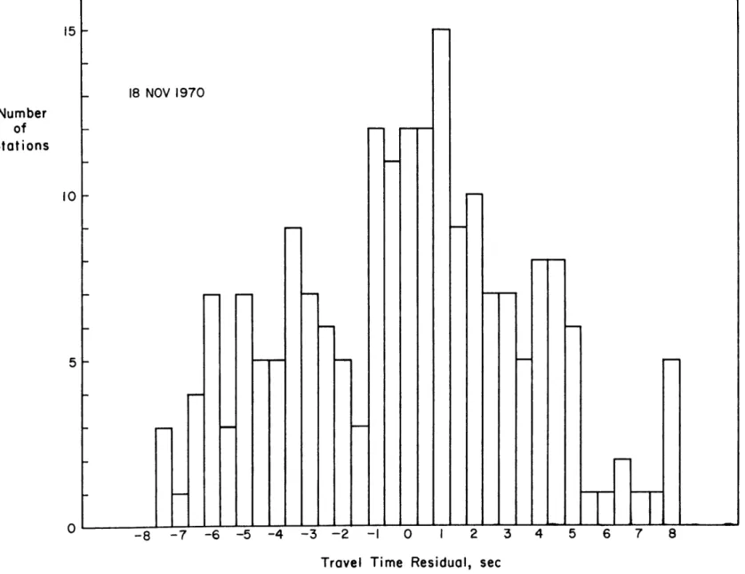
The November 18, 1970 Earthquake 80

Total Seismic Moment 82

Implications for the Oceanographer Transform 84

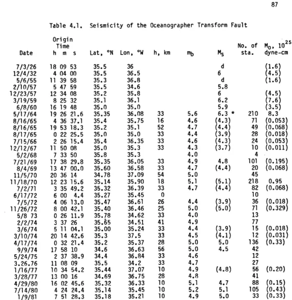
Tables 87

Figures 92

Chapter 5. Earthquakes and Tectonics of the Kane

Transform Fault . . . . . . . . . . . . . . 103

Seismicity 106

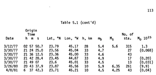
The March 12, 1977 Earthquake 107

Total Seismic Moment 109

Implications for the Kane Transform 111

Tables 112

Figures 116

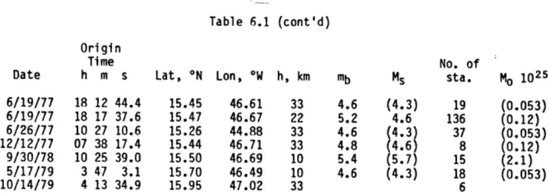
Chapter 6. Earthquakes and Tectonics of the 150 20'

Transform Fault . . . . . . . . . . . . . . . . . . . 120

Seismicity 121

The September 24, 1969 Earthquake 122

The June 19, 1970 Earthquake 125

The December 9, 1972 Earthquake 129

Total Seismic Moment 131

Implications for the 150 20' Transform 132

Tables 136

vii

page

Chapter 7. Earthquakes and Tectonics of the Vema

Transform Fault . . . . . . 149

Seismicity 152

The March 17, 1962 Earthquake 153

The May 14, 1976 Earthquake 157

The August 25, 1979 Earthquake 160

Total Seismic Moment 164

Implications for the Vema Transform 166

Tables 169

Figures 174

Chapter 8. Earthquakes and Tectonics of the Doldrums

Transform Fault . . . . . . .... . . . . 182

Seismicity 184

The August 3, 1963 Earthquake 186

The September 4, 1964 Earthquake 190

The April 4, 1977 Earthquake 193

Total Seismic Moment 195

Implications for the Doldrums Transform 197

Tables 199

Figures 205

Chapter 9. Characterization of General Seismic Behavior

of 6 Atlantic Transforms . . . . . . . . . . . . . . . 212 Comparison of Earthquake Source Parameters 212

Ms vs. mb 214

Log N(Ms) vs. Ms 216

Ms vs. Log Mo 219

viii page Summary of Results 226 Tables 228 Figures 230 References . . . . . 238

CHAPTER 1. INTRODUCTION

GENERAL CONCEPT OF TRANSFORM FAULTS

Oceanic transforms are lateral offsets of oceanic ridges,

representing a discontinuity along the ridge length of the emplacement of

crustal material beneath the ocean floor. They are recognizable by

lateral offsets in the seismicity and topographic expression of the

adjoining ridge segments, and by fracture zones, linear topographic and

magnetic features extending away from, and at right angles to, the ridge

segments. The existence of fracture zones has been known for some time,

but until 1965 they were regarded as transcurrent faults along which the

adjoining ridge segments were moving away from each other. According to

this interpretation earthquake activity should be distributed along the

entire fracture zone, and the slip direction should carry the ridge

segments away from each other, i.e., if the ridge were offset to the

right, then the direction of earthquake motion should be right-lateral

strike-slip.

Wilson (1965) noted that, according to sea-floor spreading theory,

oceanic ridges represent zones along which plates of the earth's

lithosphere move apart from each other. He therefore proposed that the

offsets of ridge axes are zones of shear between plates moving away from

the adjoining ridge segments. Wilson (1965) called this new

interpretation of the ridge offsets "transform faults". According to

this interpretation, the direction of slip during earthquakes on these

faults should be in the opposite direction to that of the ridge offset,

the seismicity along these faults should be limited to the "active"

and magnetic features which extend away from the ridge segments are

simply scars on the ocean floor produced when that crust had been part of

the active transform. By relocating and preparing fault plane solutions

for many ocean floor earthquakes, Sykes (1967) showed that most ocean

floor seismic activity was indeed limited to the "active" portion of

transform faults and that the direction of fault slip was opposite to

that of the ridge offsets, thus confirming Wilson's (1965)

interpretation. Transforms are steady-state features of constant length,

which terminate sections of active emplacement of material onto the

oceanic lithosphere and crust, and at which parts of the ocean floor with

different age are in contact. In this thesis we take a closer look at

the seismicity and source parameters of major earthquakes on several

oceanic transform faults in the north and central Atlantic in order to

characterize the motion on these transforms in space and time.

GEOLOGIC SETTING OF NORTH ATLANTIC TRANSFORM FAULTS

The general shape of the Mid-Atlantic Ridge between 50 N and 550 N,

and the locations of the major transforms in this area, are shown in

Figure 1.1. In the central and north Atlantic Ocean, transform faults

along the Mid-Atlantic Ridge range in length from less than a few tens to

several hundreds of kilometers. Common bathymetric features reported for

transform faults include a deep central trough which, at its deepest

point, can be as much as a thousand meters deeper than the surrounding

sea floor. Another feature found sometimes on one side, and sometimes on

both sides, of the transform is an elevated "transverse" ridge, running

parallel to the transform valley and forming walls which can be as much

as a thousand meters higher than the surrounding sea floor and 10 km wide

1980). The troughs typically obtain their greatest depths in depressions

located at the intersections of the transform and the adjacent ridge segments. The topographic expressions are present not only on the active portion of each transform, but extend several thousand kilometers away from the ridge into older ocean floor. The topographic features are accompanied by magnetic and gravitational anomalies.

Small-scale topographic features have been studied for a few of the transforms on the Mid-Atlantic Ridge. Detrick et al. (1973) and ARCYANA (1975) report that the inner walls of the transverse ridges flanking the active fault section of Fracture Zone A, a small transform in the FAMOUS area near 370 N, have scarps ranging in vertical offset from 50 cm to at least several tens of meters. Similar structures were reported by

Oceanographer Transform Tectonic Research Team (1980 a,b) from work of ALVIN and ANGUS on the Oceanographer transform. Schroeder (1977) reports that the inner walls of the Oceanographer transform are made up of steep, sediment-covered scarps, individually with 100 to 1000 m of vertical relief. At least for these two transforms the inner walls seem to be made up of faulted blocks of material, whose faces have considerably greater slopes than the average slope of the inner walls. Eittreim and Ewing (1975) presented results from a seismic reflection survey of the Vema transform fault, which showed that the entire valley floor was covered with thick sediment and that this sediment was cut by a fault-like feature for the entire length of the transform. The implication was that this feature is a zone along which recent

strike-slip motion has taken place. Searle (1979, 1981) presented the results of high-resolution, side-scan sonar surveys, and an analysis of the structure of the Gibbs transform using some of these data. He

concluded that the Gibbs transform was a double transform, active in the

west along the northern segment and in the east along the southern

segment. He also concluded that strike-slip activity was limited to a

single narrow zone in the center of each active segment, but that this

zone was not always delineated in the bathymetry by the location of the greatest water depth. Lonsdale and Shor (1979) examined the

ridge-transform intersection at the western end of the Gibbs ridge-transform by

mapping fault traces using a deep-tow instrument. Their results showed

that this intersection has substantial faulting along scarps running

obliquely to the spreading (or strike-slip) direction. Choukroune et al.

(1978) presented the results of dives by the C and Archemede, and concluded that (1) transforms show pure strike-slip activity with no new

crust being formed, (2) strike-slip activity is not limited to one single

well-defined fault, but (3) the zone of active strike-slip faulting is

only about 300 m to 1 km wide, and (4) the vertical relief in a

transform's large-scale bathymetry must be generated by vertical motion

along the transform flanks, and not in the zone of active strike-slip

movement.

Results have been published from several seismic refraction

experiments designed to measure the crustal structure beneath Atlantic

fracture zones. Two of these (Fox et al., 1976; Detrick and Purdy, 1980)

were on inactive limbs of fracture zones. Fox et al. (1976) found that

the basement crustal structure of the western limb of the Oceanographer

Fracture Zone consisted of an upper layer with a compressional velocity

of 4.4 km/sec and a thickness of 2.1 km, and a second layer with a

velocity of 6.5 km/sec. They did not observe any mantle arrivals, and

by assuming various velocities for the mantle. For assumed mantle compressional velocities of 7.0, 7.5, and 8.2 km/sec they obtained a

minimum thickness for the second layer of 2.5, 3, and 4 km, respectively.

Detrick and Purdy (1980) reported the results of a detailed refraction

study of the eastern inactive limb of the Kane Fracture Zone. Their

results showed the crust there to consist of only one layer over the

mantle. The layer had a compressional velocity of 4 to 5 km/sec and a

thickness of 2 to 3 km. The mantle had a compressional velocity of 7.7

to 8.0 km/sec. This result has both crustal thickness and average

crustal velocities considerably lower than those of normal ocean crust.

Ludwig and Rabinowitz (1980) reported results from a seismic refraction

and reflection experiment in the active section of the Vema transform

fault. Their results showed the transform valley to be filled with about

1500 m of sediment, and the depth to the basement ranged from 6200 to 6700 m. Below this depth they found a two-layer crust, with the first layer having a compressional velocity of 4.3 km/sec and a thickness of 2

km, and the second layer having a compressional velocity of 5.9 to 6.2

km/sec and a thickness of 2.6 km. They reported that the structure had

significant variation and that it was impossible to identify any

consistent layers with those of normal oceanic crust. Detrick et al.

(1982) presented results of a long seismic refraction experiment on the Vema transform, which showed the structure to be similar to that of the

Kane, with considerable variation, probably the result of intense

fracturing.

Solomon (1973) examined the attenuation of shear waves from a large

earthquake on the Gibbs transform and found greater attenuation for

the transform and the adjoining ridge segment than for stations whose ray

paths went elsewhere. The implication was that a zone of low Q material

existed beneath the western end of the Gibbs transform, possibly

indicating a hotspot or zone of partial melting. Rowlett and Forsyth

(1979) reported abnormally large lateral variation in P-wave travel time

residuals from a distant earthquake as observed by an array of

ocean-bottom seismometers at the western end of the Vema transform fault.

The relative magnitude and distribution of the residuals implied that

under part of the intersection of the transform and the adjoining ridge

segment there must exist a zone with lower than normal seismic velocities

which extends quite far into the mantle. They suggested that this might

be a magma chamber or a zone of partial melting. This interpretation is

similar to that of Solomon (1973).

TRANSFORM FAULT SEISMICITY

Earthquakes on oceanic transform faults have been shown to be

strike-slip and in a direction consistent with Wilson's (1965) hypothesis

of transform faults (e.g., Sykes, 1967, 1970). Isacks, Oliver, and Sykes

(1968) showed that the maximum sizes of earthquakes observed on transform faults were larger than those on oceanic ridge crests, but smaller than

those on island arc-subduction zone systems, probably reflecting the

relative amount of lithosphere in contact at each of these boundaries.

Sykes (1967) showed that transform fault earthquakes are primarily

confined to the active transform section between the adjoining ridge

segments. This finding has been verified by several experiments using

arrays of ocean-bottom seismometers (e.g., Rowlett, 1981; Project ROSE

Transform fault earthquakes generally occur at shallow depths. Weidner and Aki (1973) studied the surface waves from event pairs on the Mid-Atlantic Ridge, and found the focal depths of two strike-slip events to be 6 ± 3 km below sea floor. Project ROSE Scientists (1981) and Trehu

(1982), using a large array of ocean-bottom seismometers, found that the microearthquakes on the Orozco transform were limited to depths shallower than about 8 km.

Teleseismically determined epicenters of transform earthquakes are generally scattered over a zone that is as wide as 30 km. This may be due to poor epicentral determinations or it may indicate that seismic activity is distributed over a broad area. Epicenters determined by Project ROSE Scientists (1981) for the Orozco transform were divided into two groups. One group, near the western end of the transform, showed clear alignment along a narrow trough parallel to the slip direction between the Cocos and Pacific plates, and the first motions of these events were consistent with strike-slip faulting along the transform. The other group occurred near the center of the transform, in a topographically complicated region, and did not show any preferred alignment with the strike of the transform. One interpretation is that the microseismicity is composed of both strike-slip activity and other activity, possibly related to topographic features. This would be consistent with the interpretation of Eittreim and Ewing (1975) that the linear feature they observed in the sediments of the Vema transform

represented a narrow zone of stike-slip motion. Microearthquakes at the ends of transforms on slow spreading ridges do not exhibit alignment with the transform strike, but instead are generally scattered across a

(Rowlett, 1981), which suggests that many of these events are related to

processes unique to the intersection zone.

There is evidence that the size of transform fault earthquakes is

related to the dimensions and slip rate of the transform. Burr and

Solomon (1978) found that (1) the maximum seismic moment for such

earthquakes decreases with slip rate and increases with transform length

up to lengths of about 400 km, (2) average fault width increases with

transform length and decreases with slip rate, and (3) larger earthquakes

generally occur toward the center of a transform. They interpreted these

results as indicating that the lower boundary of seismic activity is

defined by an isotherm, conservatively determined to be between 50 _{C and}

3000_{C. This is consistent with the finding of shallow focal depths for}

transform earthquakes.

LARGE EARTHQUAKES ON NORTH ATLANTIC TRANSFORMS

Comparatively few large earthquakes on oceanic transform faults have

been studied in detail. For the north and central Atlantic, several

studies may be noted. As mentioned above, Weidner and Aki (1973)

inverted Rayleigh wave amplitude and phase spectra to obtain the source

characteristics of two strike-slip earthquakes from North Atlantic

fracture zones which occurred on May 17, 1964 and June 9, 1970.

Epicenters of these events were 35.29* N, 36.07* W, and 15.40 N, 45.9* W,

respectively. Both of these events had mb = 5.6. Weidner and Aki (1973) found seismic moment values for these events of 1.03 x 1025 dyne-cm and

1.94 x 10 dyne-cm, respectively. Udias (1971) studied the Rayleigh

wave spectra of four earthquakes, two of which were on a transform fault

system we have studied here, which we call the Doldrums transform fault.

moment for these events. Sykes (1967, 1970) presented fault plane solutions for several North Atlantic earthquakes, which showed the expected strike-slip motion. Tsai (1969), Wyss (1970), and Dziewonski and Woodhouse (1982) determined seismic moments for various transform fault earthquakes.

Kanamori and Stewart (1976) performed a detailed study of the

surface waves and body waves from two earthquakes on the Gibbs transform which occurred on February 13, 1967 and October 16, 1974. They found seismic moments for these events of 3.4 x 1026 dyne-cm and 4.5 x 1026 dyne-cm, respectively. By assuming bilateral rupture propagation, they found fault lengths of 60 km and 72 km. With these values and assuming a fault width of 10 km, they found displacements of 160 cm and 180 cm and dislocation velocities of 23 cm/sec and 18 cm/sec, respectively. An important implication was that these events exhibited slower than normal fault movement and therefore excited much greater long-period surface waves than usual for events of this mb. By comparing the displacements and fault lengths of these events to the total length of the transform and the rate of slippage predicted by magnetic anomalies, and by assuming that previous large earthquakes on the transform were similar to these, they concluded that the Gibbs transform slips in a jerky manner, with major events alternating between the eastern and western half. The time for one complete cycle is about 26 years, with the entire transform slipping once during this period.

OBJECTIVES OF THIS STUDY

Previous work on transform fault earthquakes has shown them to be strike-slip, reflecting the relative motion of plates across the

(1978) showed that there is some connection between a transform fault's dimensions and slip rate and the earthquakes which occur on the

transform. From the study of Kanamori and Stewart (1976), the

earthquakes gave us some clues as to how the Gibbs transform behaves,

although the earthquakes themselves seemed to be somewhat unusual.

In this work we examine the seismicity and largest earthquakes of

several North Atlantic transforms. Our goal is to try to understand

plate slip along these transforms, and in particular to focus on the

following questions: What are the main source parameters of the large

earthquakes? How deep in the crust or mantle do they occur? Are other

earthquakes similar to those on the Gibbs transform studied by

Kanamori and Stewart (1976)? Do transform earthquakes exhibit abnormally

high or low stress drop or displacement? Do transforms slip smoothly or

do they move in discrete, jerky episodes? What is the repeat time for

seismic episodes on any section of a transform? Have entire transforms

slipped at least once during the known seismic history? Is there

agreement between the total seismic moment observed on any transform and

that predicted by the slip rate and fault dimensions, or has the observed

seismic activity been too uneven for such comparisons to be reliable?

To try to answer these questions we have constructed synthetic

seismograms for comparison to the observed P waveforms from the large

earthquakes on five North Atlantic transforms (Oceanographer, Kane, 150

20', Vema, Doldrums). The technique adopted for P-wave synthesis is

described in Chapter 2. On the basis of the P-wave modeling we have

determined source parameters for twelve earthquakes. We have also

combined data from the known seismicity of these five transforms plus the

11

estimate the observed seismic slip rate, for comparison to the rate of

slip predicted from magnetic anomalies. The results are presented in

Chapters 3 through 8 of this work. Finally, in Chapter 9, we examine the

similarities and differences between the transforms studied and the

Figure Captions

Figure 1.1. The Mid-Atlantic Ridge and other plate boundaries between 50

N and 550 N, and 150 W and 550 W. The major transform faults on the

Mid-Atlantic Ridge are also indicated, and labelled G for the Gibbs transform, 0 for the Oceanographer transform, K for the Kane

transform, F for the 150 20' transform, V for the Vema transform, and D for the Doldrums transform system. This represents an interpretation of the bathymetry taken from Uchupi (1982). The plate boundaries marked with question marks are not well-known. The multiple-transform interpretation of the Gibbs and Doldrums

13

G

50

N.American plate Azores

400

O

0

-30

K

N

D

50

40

30

20 W

CHAPTER 2. METHOD OF P-WAVE SYNTHESIS

GENERAL TECHNIQUE

We have constructed synthetic seismograms of the P-waves for

comparison with the observed seismograms from the largest strike-slip

earthquakes on the transform faults treated in this study. By matching

the synthetic waveforms and amplitudes to observed ones we have been able

to determine some of the source parameters and other features of these

events.

We have used the method of Langston and Helmberger (1975), used also

by Kanamori and Stewart (1976) and Chung and Kanamori (1976), with some modifications of our own. The basic approach is a time-domain

superposition of the direct P, pP, and sP phases. The pP and sP phases

are delayed by an amount appropriate to the event depth and adjusted in

amplitude by the reflection coefficient for the top of the oceanic crust.

The amplitude of each phase is corrected for the radiation pattern of the

event, and the final time series is corrected for geometric spreading,

attenuation, instrument response, and the effect of the free surface near

the receiver.

The far-field displacement for a double-couple point source in a

uniform, unattenuating medium can be expressed by (Love, 1934)

up(t) = 1 A(t-r/v) Re, (2.1)

47Tpv3

where r is the distance, p is the density, v is the wave velocity, R6,0 is a factor for the radiation pattern, M is the time derivative of the

seismic moment, and t is time. We can think of M as the rate of

generation of seismic moment. If we express

A

where Mo is the.scalar seismic moment and T(t) is a time series such

that

f

then T(t) represents a normalized displacement function with the same

shape as would be observed as a direct P wave at teleseismic distances.

The far field displacement expression (2.1) then becomes

up(t) = 1 M0 Re.3 T(t-r/v). (2.4)

4irpv3

P-wave arrivals on observed seismograms are composed principally of

the direct P and the surface reflections pP and sP. We can express these

reflected phases by using the appropriate radiation pattern factor Re.0 multiplying by the free surface reflection coefficient A(ir), where ir

refers to the emergent angle at the point of reflection for the phase i,

and then delaying each phase At for the extra travel path length due to

the event depth. The complete waveform is then the sum of these phases

and can be expressed as

u(t) = 1 M0 (T(t-r/v) R, + T(t-r/v-At₂) R₂ A₂

47rpv3

+ T(t-r/v-At₃ ) R₃ A₃) (2.5)

where the subscripts 1, 2, and 3 refer respectively to the P, pP, and sP phases.

To obtain the final synthetic seismogram we correct this expression

for geometric spreading, attenuation, crustal effects at the receiver,

and instrument response. The result can be expressed as

usyn(t) = u(t) g(A,h) C(io) * F(t/t*) * I(t) (2.6)

a t*

where a is the radius of the earth, g(A,h) is the geometric spreading

factor, C(io) is the free surface effect at the receiver, io is the

is the instrument response, * denotes the convolution operation, A is the epicentral distance to the station, h is the focal depth, and t* is the

attenuation parameter, defined as the ratio of travel time to the average

quality factor Q along the ray path.

Several of the factors in the above expressions have been given in

previous work. The radiation pattern factors (Ri's) have been given by

Kanamori and Stewart (1976). The free surface correction C(io) is given

in Bullen (1965). The geometric spreading factor g(A,h) is given by

Kanamori and Stewart (1976) as

g(A,h) =

(

Po00 sin A cos l0 dA I

where the subscripts h and o refer to the source and receiver,

respectively. The incident angles for this expression were calculated

using travel times from Herrin (1968) and the velocity appropriate to the

depth for the source structure, and using a velocity of 6.0 km/sec for

the receiver. The attenuation function F(t/t*) corresponds to a linear,

causal, constant-Q, slightly dispersive earth model calculated by

Carpenter (1966) from the work of Futterman (1962) and Kolsky (1956).

[The paper of Carpenter (1966) has been reprinted by Toksoz and Johnston

(1981).] The instrument response correction I(t) is taken from the

frequency domain correction given by Hagiwara (1958). The reflection

coefficients Ai are given in Ewing et al. (1957), though for potential

amplitude rather than displacement amplitude. This makes no difference

for the pP conversion. For the sP conversion however it means that we

must also use the additional factor of

a Cos i

Bsp = c p (2.8)

where a is the P-wave velocity and a the S-wave velocity in the medium where the reflection takes place, is is the S-wave incident angle on the

surface, and ip is the emergent angle of the reflected P-wave. Thus the

sP term in (2.5) becomes T(t-r/v-At,) R₃ A3 Bsp. For all of these

calculations and for the velocity models used we have assumed a Poisson

solid, i.e., (a/s)2 = 3.

The scalar moment is a factor which (along with several other

factors) multiplies the source time function to produce the amplitudes of

the final waveform. Thus the moment represents a scaling factor for the

synthetic seismograms. To determine the seismic moment for an earthquake

we first determine, for each station used, the moment necessary to

duplicate in the synthetic waveform the amplitude of the observed

waveform. (For most seismograms presented in the following chapters,

this was the zero to peak amplitude of the first major signal

displacement. For the waveforms which had small first arrivals followed

by larger signals with opposite polarity, we usually used the amplitude of this second peak.) We then average these values to find the seismic

moment of the earthquake, using the formula

ln Mo = 1/n 2 ln Moi (2.9)

where n is the number of stations used and Moi is the moment for station

i which gave the same amplitudes for the observed and synthetic

seismograms. Using this approach also allows us to express the scatter

in the observed Moi's by determining the standard-deviation a of ln MO;

thus exp (a) represents an "error factor" for Mo.

If we have any information about the fault dimensions, we can then

determine the displacement D and particle velocity Vt for each earthquake using the formulas

M= y L w D and Vt = D/Rt,

and we can determine the stress drop for each earthquake using the

formula given by Kanamori and Anderson (1975) for a strike slip event

Aa = 2 (2.10)

ff w

where y is shear modulus of the material, D is the average displacement, w is the fault width, L is the fault length, and Rt is the rise time.

MODIFICATIONS

We have made two improvements to the previously used versions of

this method for P-wave synthesis. The first is the use of a layered

velocity structure near the source. In previous applications of this

technique (e.g., Kanamori and Stewart, 1976) the structure near the

source was assumed to be a simple half-space. In order to improve the

accuracy of the focal depth determination we used a layered structure, in

which the actual properties of the faulted material depend on the layer

in which the event occurred. The calculation of the delays Ati for the

pP and sP phases were made by tracing the reflected P from the depth of the focus up to the surface and then, as the original s or p phase, back

down to the source, changing the emergent angle at each interface

encountered. The final delay value was a summation of a path-length

component for each layer (accounting for the extra travel path of the

reflected phases), and a horizontal component (accounting for the

slightly smaller epicentral distances traveled by the reflected phases to

the station from the point where they reached the depth of the focus).

The total delay value for either the upward or downward direction can be

given by the expression

At = E hj (1/(vj cos ij) -(tan ij)/p) (2.11) 3

where hj is the thickness of layer

j,

j,

j,

velocity for that epicentral distance and event depth.

In practice this summation over the

j

reflection at the surface. For the complete pP delay time this value is

doubled, since the upward-going p phase follows a similar path, with

similar incident angles at each interface, as the reflected pP. However

for the sP phase we must trace the s ray path back down from the point of

reflection to the same depth as the focus. Since the s to P conversion

requires a difference between incident and reflected angles we use an

incident angle appropriate for the s phase. This results in different

incident and refracted angles at each interface, so that the horizontal correction for the sP phase is what would be appropriate for a ray from a virtual source slightly closer to the receiver than the actual source.

Figure 2.1 illustrates the geometry of these corrections. (For these

calculations we have assumed that the pP and sP phases reflect off the

basement-sediment interface, not the sediment-water interface; except

possibly for transforms with large sediment thickness, the former is

probably the stronger reflector. Thus the water depths used include

actual water depth plus sediment thickness.)

The other modification we have introduced is the use of a finite

fault, and the resulting variation of the apparent source time function

T(t) with emergent angle and station azimuth. We assume that rupture

begins at the event focus and propagates horizontally for some finite

distance with a constant rupture velocity. We allow the fault to be

two arms of the fault are of equal length. We can then calculate the angle Q between the propagation vector and the ray to any station i by

cos Qi = cos 6 cos di + sin 0 sin di cos $ cos Azi

(2.12)

+ sin 6 sin di sin Azi sin

*,

where Azi and di are the azimuth measured clockwise from north and

emergent angle measured up from vertical, respectively, for the ray to

station i, $ is the azimuth of the propagation vector, measured clockwise from north, and 6 is the angle of the propagation vector measured from

vertical. This geometry is illustrated in Figure 2.2. We assume for all

cases treated here that propagation occurs horizontally along the strike

of the fault, so that 0 = w/2. Equation 2.10 thus reduces to cos Qi = sin di cos ($ -Azi). (In Figure 2.2 we also show the fault dip 6. The

fault dip is used in determining the effect of finite fault width on the

source time function.)

The apparent propagation time Ti, as seen at station i, for any

unilateral event with fault length L and rupture velocity vr will be

Ti = L (1/vr - (cos Qi)/v). (2.13)

As shown in Figure 2.3, this represents the propagation time plus (or

minus, depending on the propagation direction) a correction for the extra

path length required by source finiteness. For a bilateral fault the

result will simply be the superposition of two simultaneous equal-length

unilateral faults propagating in opposite directions. This method is

similar to that used by Bollinger (1968) in examining source finiteness

and directivity in the P waves from several large earthquakes, including

one event studied here.

The time function corresponding to this apparent propagation time is

rise time of the displacement, and the other representing nearly

instantaneous rupture along the fault width. The rise time function is

taken as a boxcar function, with a duration equal to the rise time. The

fault width function is calculated in the same manner as the propagation

time function Ti, except that fault width replaces fault length and vr is assumed to be infinite in Equation 2.13, and Qi is taken from Equation

2.12 with n/2-6 replacing 0. Examples of source time functions for P,

pP, and sP phases from a vertical fault, with dimensions similar to those required by the earthquakes studied in the following chapters, are shown

in Figure 2.4. Our approach assumes that the fault plane exists in a

medium characterized by a single seismic velocity even though the plane

may span several layers.

As a result, the apparent source time function, and therefore the

waveform, of the synthetic seismogram for each station varies with the

emergent angle and azimuth of the ray to that station. This effect can

be important for horizontally propagating faults (including large

transform fault events), particularly for unilateral rupture. Figure 2.5

shows, for four different depths, a pair of synthetic seismograms, each

of which includes one calculated using bilateral rupture and one assuming

unilateral rupture in a direction away from the station. All other fault

parameters were held constant for each pair. The effect of rupture

direction, as well as that of focal depth, can be seen clearly.

THE PROBLEM OF FINITE WIDTH

The time function for fault width implies essentially infinite

propagation of the rupture along one dimension of the fault, or in other

words, horizontal propagation of a vertical line source. We realize that

but there is not enough precision available in the shape of observed

P-waves to justify a more detailed model. There are two significant

objections to our approach that can be raised, however. One involves the

calculation of the pP and sP delay times for a horizontally propagating

fault. For our model of horizontal rupture along a nearly vertical

fault, the initiation of rupture is assumed to take place simultaneously

along a vertical line. This means that the up-going pP and sP waves

begin at a different depth from the down-going direct P. If, for

example, the fault has a width of 4 km and extends from the surface down

to 4 km, then the pP and sP phases would arrive at a receiver

simultaneously but behind the direct P phase by roughly the time required

to travel vertically the extra 4 km. Such a situation is not likely

because the initiation of rupture is more likely to occur at a point than

along a line, and this point can be located anywhere along the fault's

width. We therefore assume that the focal depth is a point source rather

than a line source for the purposes of calculating the pP and sP delay

times. This means that we should use, for our "fault width" convolution

of the source time function, some non-rectangular function which

represents the build-up of rupture away from the point of origin into the

line source which will ultimately propagate horizontally. This would

require, as noted above, the inclusion of a correction for wave shape

which cannot be resolved from the shapes of observed P-waves. Therefore

we have not included this additional complexity, even though we realize

it introduces an incompatibility between two facets of our model.

The second major objection to this treatment of the fault width is

more serious, and tends to obscure one of the major ambiguities inherent

line at a finite rupture speed, then the width function can be calculated using Equation 2.13, with fault width substituted for fault length, or

Twi = w (1/vr ± Icos Qil/v). (2.14)

For the P phase, if the rupture is upward the + sign is used, and if

down-ward, the -sign is used. For the pP and sP phases the signs should be

reversed. The actual contribution of the fault width to the source time

function is probably different from what we calculate using infinite vr-We can estimate the magnitude of this difference by assuming that

the rupture speed approximately equals the shear wave velocity, so that

vr v / /, and by noting that the emergent angles, and therefore the

angle Qi in Equation 2.14, are usually around 30* for the stations used

in this study. Thus, for the P phase, the minimum value possible for Twi

is about 0.5 w/vr, corresponding to downward rupture, and the maximum

value possible is about 1.5 w/vr, corresponding to upward rupture. Since

we determined the width effect by using Twi = w (cos Qi)/v, the actual fault width might have been as large as the value we used or as little as

1/3 of the value we used, depending on whether rupture propagated downward or upward, respectively. Since the pP phase emerges from the

source upward rather than downward, the effect of vertical rupture on the

pP time length will be opposite to that of the P, i.e., if we have

estimated the duration of the width component of P correctly (actual

downward rupture), then we will have underestimated the duration of the

width component of pP by possibly a factor of 1/3. If the fault actually

ruptured upward, the duration of our width contribution to P and pP could

be wrong by a factor of 1/3 and correct, respectively. If we conjecture

that an upper limit on the ratio of vertical rupture time to horizontal

then the duration of either the P or pP might therefore be underestimated

by a factor of 2/3, as a worst case. Since each component is normalized

to have f T dt = 1, then the maximum amplitude of either component may be overestimated by this much also.

For the sP phase we have vr m v, so that our calculated Twi may be

underestimated (and therefore w overestimated) by a factor of 1/2.2 for

downward rupture (remember that sP emerges from the fault upward), while

for upward rupture, our calculated Twi may be overestimated by (and

therefore w underestimated by) a factor of 6.5. Our calculated total

duration of any sP phase may therefore be in error by a factor of perhaps

2 either larger or smaller, and likewise any sP amplitude. If rupture is

bilateral vertically, with rupture starting in the center of the fault

plane and propagating with a constant vr, then there would be two equal

components to the sP phase, with the upward propagation component from

the top half of the fault having possibly 1/4 the duration and 4 times

the amplitude of the part from the bottom half of the fault. With such a

larger amplitude the top half component would probably dominate the

waveform, and thus the actual fault width could be twice that indicated

by the sP components of our synthetic seismograms.

Exactly what all of this does to any comparison between synthetic

and observed waveforms probably varies with each event. Since the sP

component usually has the larger amplitude it probably dominates the

observed waveforms, and this effect may be major. For those events

presented later which have slightly non-vertical fault planes, the effect

may depend on the azimuth of each station. Clearly upward rupture is

limited by the distance from the focal depth to sea floor, so that actual

bilateral vertical propagation. However, since seismic velocities

increase with depth, rupture speeds may increase also, so that equal-time

bilateral rupture may occur even though the lower (and therefore not as

significant) portion of the fault may be larger than the top portion.

The result is that, for the important sP phase, and to a lesser extent

for the P and pP phases, an actual fault width may easily be more than

twice the distance between the focal depth found and sea floor, if the

vertical rupture was bilateral.

The nature of the spread of rupture over a finite fault can

significantly affect the shape of the waveform produced. This fact

should be considered whenever synthetic seismograms are constructed, and,

in particular, whenever fault dimensions are inferred from source time

functions. Obviously fault width cannot be clearly resolved by this

method because the observed waveforms do not contain enough information.

More importantly, fault orientation cannot be resolved as precisely as it

would first seem because the relative sizes of the three main phases can

vary with fault dimensions and the shape of the spread of rupture as well

as with fault orientation. Even for synthetic seismograms calculated

using a single source time function for all three phases, care must be

exercised when fault dimensions are inferred because the source time

functions of real earthquakes are probably not the same for these phases,

and, in addition, the effects of the fault dimensions on source time

functions are ambiguous. This problem exists with synthetic seismograms

generated using any method, not just the one used here, and it will

remain a problem until the nature of the rupture process is better

understood.

These fault width effects are significant because they offer

in the later chapters. One such feature is that the events presented all

seem to have had time functions of 5 to 10 sec, even though the seismic

moments varied by nearly two orders of magnitude. In order to produce

these short time functions our model required small fault dimensions and

thus produced very large displacements for the larger events. The

possibility that the fault widths are larger than estimated means that

the displacements may be overestimated; the effects discussed here offer

an explanation of how events with very different seismic moments

(corresponding to very different fault dimensions) might have similar

(and short) time functions.

Another feature is that many of the events studied had some sort of

precursor phase. One way to generate a "precursor" is to have a small P

compared to pP and sP, a condition which can occur for some stations with

a strike-slip earthquake if the fault plane is almost, but not quite,

vertical. However, if the rupture was vertical and primarily upward,

then the P phase could be quite long and therefore have a small

amplitude, while the pP and especially the sP phase could be short and

impulsive, producing a "precursor" effect with a completely vertical

fault plane. Figure 2.6 shows two synthetic seismograms, one constructed

using horizontal rupture propagation on a non-vertical fault, the other

using upward rupture propagation on a vertical fault. For the amplitudes

to be the same, the former required a seismic moment that was roughly 1.5

times that of the latter. The two waveforms also required different

source dimensions so that the displacement inferred for the former was

about 2.5 times that inferred for the latter.

The hypothesis that rupture begins below the surface and moves

most of these events had focal depths several km below the sea floor, thus allowing room to rupture upward. These possibilities will be

discussed later but are presented now also in order that the lack of

resolution of fault width be clearly understood.

CHECKS ON THE VALIDITY OF THE METHOD

As a check of our method, we computed synthetic seismograms of P

waves and compared them to the results of Langston and Helmberger (1975).

For this comparison we used their source velocity structure, which

consisted of a half-space with a seismic velocity of 6.0 km/sec and a

density of 2.7 g/cm3. We computed seismograms for a strike-slip

earthquake, as observed at a station with an epicentral distance of 80*

and on an azimuth 450 from the strike of the fault. We used two sets of

source dimensions and rise times, which produced the source time

functions given by Langston and Helmberger (1975) as representing a low

stress-drop earthquake and a high stress-drop earthquake. This was a

trapezoidal time function, with a rising ramp of 0.5 sec duration, a

plateau of 1.5 sec duration, and a falling ramp of 0.5 sec duration for

the high stress-drop case, and values of 2.0 sec, 6.0 sec, and 2.0 sec,

respectively, for these variables in the low stress-drop case. Synthetic

seismograms were computed for focal depths of 5, 10, 15, and 20 km. The

resulting waveforms are shown in Figure 2.7 and are practically identical

to the waveforms given in Figure 4 of Langston and Helmberger (1975).

For the oceanic earthquakes studied here there were also phases of p

waves traveling upward through the 4 to 5 km of water over the transform

fault, reflecting off the water surface, and traveling back down. These

reflections do not influence the first 15 seconds of so of each

down through the water. We do not include these water reflections in our synthetic seismograms. The observed waveforms presented in all of the

following chapters have complexities after the first 15 sec or so, which

we have been unable to duplicate in synthetic seismograms. We have

assumed that these complexities are due partly to water reflections, and

we have not given these details much consideration when matching

waveforms.

The primary limitation to our method is that we do not include any

phases or reflections other than P, pP, and sP. For most earthquakes

complexities in the signal are introduced by the layered velocity

structure near the source; reflections and phase conversions at the

interfaces can introduce other phases into the final waveform. One such

complexity is presence of pP and sP reflections at the sediment-water

interface as well as the basement-sediment interface, particularly for

transforms with an unusually thick cover of sediment like the Vema. The

reflections and phase conversions at the interfaces in the oceanic crust

generally do not contribute much to observed waveforms, because the

amplitudes are too small. Figure 3-16 in Ewing, Jardetsky, and Press

(1957) shows that, for a typical interface in an oceanic crust, the

amplitude ratios of reflected or transmitted P waves from incident SV

waves are only about .05 to .07 for the range of emergent angles used

here. Figure 3-15 in Ewing, Jardetsky, and Press (1957) shows that for

these interfaces and emergent angles the amplitude ratio of reflected P

waves to incident P waves is less than .05. Another factor which would

minimize the contribution of internal reflections in the layers of an

oceanic crust is that the Q values for these layers may be fairly low;

thus would have amplitudes even further reduced compared to the P. pP,

and sP phases. The amplitudes of internal reflections would of course be

increased if multiple reflections were superimposed with constructive

interference. The magnitude of this effect would be dependent on the

predominant period of the signal, layer thicknesses, and the angle from

vertical of the emergent ray to each station; thus the effect could vary

for each station and for each earthquake. These phase conversions and

reflections could be included in our method, but it would contribute to

the computational complexity which we have tried to minimize.

Another source of waveform complexity is the contribution introduced

by a layered velocity structure beneath each receiver. We did not try to correct for this because each receiver would have its own structure.

Other methods of constructing synthetic seismograms have been

developed which involve superposition of eigenfunctions in wavenumber

space, e.g. Bouchon and Aki (1977). One major difference in the two

techniques as applied to a layered structure for a transform fault is

that the wavenumber superposition method includes all of the internal and

water reflections, and phase conversions, expected for the structure, as

discussed in the preceeding paragraph, and thus represents a complete

solution. However our method offers the advantage that it is numerically

simpler and requires less computer time. Because our method is a time

domain synthesis, it is easier to understand the contribution to the

result from each of the fault parameters, and to adjust these parameters

to bring about the desired result.

We have prepared synthetic seismograms using both techniques, for

(1) a simple half-space, (2) a layer of water and a crustal layer over a

layer over a half-space, with the event focus in the mantle. The

comparisons, given in Figures 2.8 and 2.9, show that the waveforms

calculated from the two methods are quite similar, though the agreement is

best for the simple half-space model. For each figure, all of the

seismograms are plotted with the same vertical scale, so that the

amplitudes calculated with the two methods could be compared. The maximum

amplitudes found with each method for the half-space model differed slightly, but this was primarily due to different methods of calculating

the geometric spreading factor. (This calculation involves taking the

second derivative of the travel-time tables and thus is subject to

numerical "noise".) When the amplitudes were corrected for this effect,

the difference was no greater than 1%. The slight dissimilarity of

waveforms for the other structures is presumably indicative of the effect

produced by not including all reflected phases in our method. It must be

remembered that the comparisons shown here for the layered structures are

not valid for other combinations of focal depths, source time functions,

and layer dimensions, since the interference between multiple reflections

depends on these parameters. In particular the effect of the water layer

shown in Figure 2.9 cannot be taken as representative of the effect for

all transform fault earthquakes.

PARAMETERS AND DATA NEEDED

With our method the following independent variables must be given:

P-wave velocity and density for each layer in the structure near the

source, station azimuths and distances, event depth, fault strike and

dip, slip angle, fault length and width, rise time, rupture velocity,

propagation direction (bilateral or unilateral and, if unilateral, which