Dynamics of disturbances on the intertropical convergence zone.

DYNAMICS OF DISTURBANCES ON THE INTERTROPICAL CONVERGENCE ZONE

by

JOHN RAPHAEL BATES

B.Sc., National University of Ireland (University College Dublin)

(1962)

SUBMITTED IN PARTIAL FULFILLMENT OF THE REQUIREMENTS FOR THE DEGREE OF DOCTOR OF PHILOSOPHY

at the

MASSACHUSETTS INSTI1UTE OF TECHNOLOGY September, 1969

Signature of

Auhor...Department o Meterology,

0. -eLQoe

~ ~ ~ ~ ~ ~

ee Ia o eo e IFe eo September

9,

1969 Certified by ... . ... .... . ... .

Sbs Supervisor

Accepted by ...

Chairman, Departmental Committee on Graduate Students

WTLI !

EAWN

MI

FRARI

S

DYNAMICS OF DISTURBANCES ON THE INTERTROPICAL

CONVERGENCE ZONE

John Raphael Bates

Submitted to the Department of Meteorology on September 4, 1969 in partial fulfillment of the requirements for the degree of Doctor of Philosophy.

ABSTRACT

The dynamics of disturbances on a theoretically derived In-tertropical Convergence Zone are studied.

Radiative cooling over a hemisphere is parameterised by a Newtonian cooling law, relative to a radiative equilibrium temper-ature which decreases from equator to pole. Release of latent heat of condensation in the tropics is treated as a function of convergence in the planetary boundary layer.

The zonally symmetric field of motion which evolves in res-ponse to these sources of energy shows a concentrated region of rising motion near, but not at, the equator. The associated low-level wind field possesses a strong cyclonic shear.

Asymmetric perturbations periodic in longitude are introduced by means of truncated Fourier series. The wavelengths are chosen to correspond to maximum instability in the ITCZ, and as such are too small to permit baroclinic instability in middle latitudes. In this way, the stability of the low latitude flow is examined while excluding middle latitude perturbations.

The low-level wind field in the vicinity of the ITCZ is found to be barotropically unstable, the wavelength of maximum growth rate being about 2000 km. The corresponding e-folding time is found to be of the order of two days, depending on the frictional and heating coefficients.

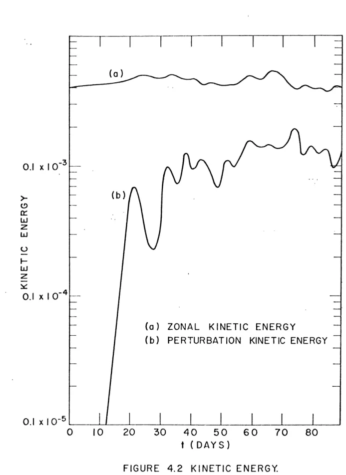
The perturbations are allowed to grow to finite amplitude. In the initial stages of growth, the Reynolds stresses supply most of the perturbation energy. At the mature stage, the energy is provided mainly by direct conversion of condensationally produced eddy available potential energy. Further growth is then limited by frictional dissipation of kinetic energy.

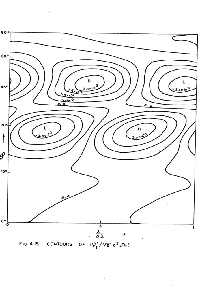
The mature disturbance shows a highly asymmetric cell of concentrated rising motion, bounded by regions of weak sinking motion, propagating towards the west at about 13 kts. The dis-turbance is 'warm-core', having a much larger amplitude at the lower than at the upper level.

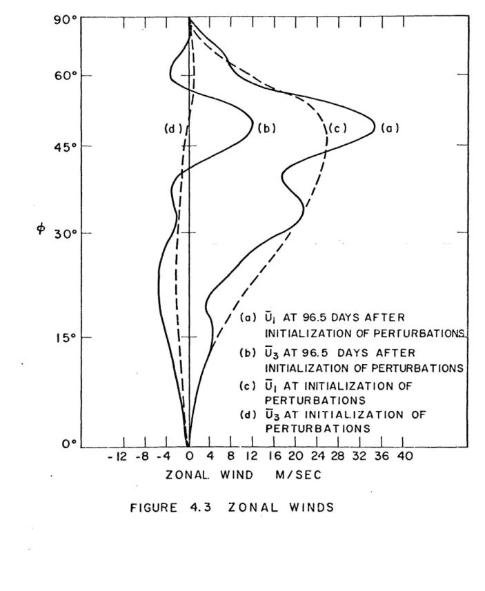
The mean flow is in turn influenced by the disturbance through the mechanisms of Reynolds stresses, eddy conduction and the modi-fication of the mean flow condensational heating through boundary-layer pumping. The influence is seen on the mean temperature and zonal wind fields, and may extend to latitudes poleward of where the perturbation amplitude in situ has decreased to zero.

A framework is thus provided for viewing tropical disturbances as an integral component of the general circulation of the

atmosphere.

Thesis Supervisor: Jule G. Charney Title: Sloan Professor of Meteorology

DEDICATION

5

ACKNOWLEDGEMENTS

The'author wishes to express his gratitude to Professor Jule Charney, under whose guidance this work was accomplished, and whose boundless enthusiasm was a constant source of encouragement.

He also wishes to thank Professor Norman Phillips who was always willing to help when the need arose.

Miss Diana Lees provided invaluable assistance with the pro-gramming and with the preparation of the diagrams, Miss Isabelle Kole did excellent work with the figures, and Mrs. Karen MacQueen was a most proficient typist. To all three, the author expresses his appreciation.

Much of the computing was performed at the NASA Institute for Space Studies in New York. Thanks are due to Dr. Robert Jas-trow for making these facilities available and to Mr. Charles Koh for help in running the program.

During the first three years of his stay at M.I.T., the author was the recipient of a Ford Foundation Fellowship, and for the final two years of a Research Assistantship made possible by Grant Number GA-402X from the National Science Foundation. To both of these organizations he is greatly indebted.

Finally, he wishes to express his appreciation to the Di-rector of the Irish Meteorological Service for the generous grant of special leave for the duration of his graduate studies.

TABLE OF CONTENTS

Chapter 1 INTRODUCTION 15

Chapter 2 THE MATHEMATICAL MODEL 23

2.1 The two-level model 23

2.2 The mean equations 28

2.3 The perturbation equations 36 2.4 Parameterisation of the heating 43 2.5 Spectral resolution of the

per-turbation equations 50

2.6 The governing equations in

di-mensionless form 58

2.7 Algorithm for solving the equations 68

Chapter 3 LINEAR DYNAMICS OF THE PERTURBATIONS 79

3.1 The linearised equations 79

3.2 The baroclinic case 83

3.3 The case with condensational

heating 87

3.4 A special case of barotropic

instability 90

Chapter 4 SOME PRELIMINARY EXPERIMENTS 96

4.1 The case of zero condensational

heating 96

4.2 The zonally symmetric ITCZ 107

Chapter 5 DISTURBANCES ON THE ITCZ 123

5.1 Single-wave perturbations without

friction and condensational heating 123 5.2 Single-wave perturbations with friction

but without condensational heating 130 5.3 Single-wave perturbations with

friction and condensational heating 133 5.4 Multiple-wave perturbations with

heating and friction 137

Chapter 6 SUMMARY AND CONCLUSIONS APPENDIX BIBLIOGRAPHY BIOGRAPHICAL SKETCH 181 189 199 203

8

DEFINITIONS OF SYMBOLS

Variables and Constants - Roman Alphabet

OL = mean radius of the earth

aj = wave number for jth spectral component

A

= Austausch coefficient

C = phase speed

C = dimensionless ground friction coefficient for mean flow

C = drag coefficient

C = coefficient of specific heat at constant pressure

= scaling magnitude for the wind

p = characteristic magnitude of w used in 4

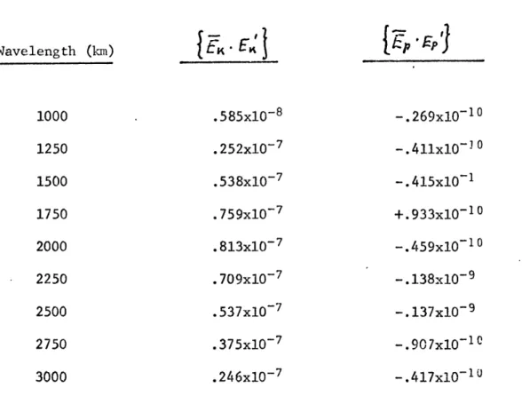
Ex. = dimensionless mean kinetic energy

Ex = dimensionless perturbation kinetic energy Ep = dimensionless eddy conduction of heat

Ep = dimensionless mean potential energy

Ep = dimensionless perturbation potential energy

= Coriolis parameter 2Ssin9)

I

Coriolis parameter at central latitude for perturbations

I=

smoothing function for condensational heating

Fj(X)= spectral component

Fj = frictional force per unit mass in eastward direction

F,

= frictional force per unit mass in northward direction = acceleration of gravity

= unit vector in eastward direction

3

= number of spectral (sine and cosine) components used in expansion of perturbation quantities

K = unit vector in vertical direction Al = internal friction coefficient

K(

= dimensionless lateral viscosity coefficient K = dimensionless internal friction coefficient K = dimensionless radiational cooling coefficient K = dimensionless ground friction coefficient for the

perturbations

L

= basic linear periodicity at equator

LL

= scale length

= angular momentum per unit mass

= pressure

= 1000 mb

= specific humidity

= rate of heat addition per unit mass

GL

= dimensionless condensational heating function

= distance from earth's centre = gas constant for dry air

g

= Richardson number

o = Rossby number

= dimensionless difference of Reynolds stresses at upper and lower levels

~p = dimensionless sum of Reynolds stresses at upper and lower levels

t

= time

= absolute temperature ... also dimensionless temperature relative to radiative equilibrium value at the equator T^ = equator to pole difference of radiative equilibrium

U4

= component-of velocity in eastward direction

L

= dimensionless sum of eastward velocities at upper and lower levels

= representative value of low level wind speed

= component of velocity in the northward direction

V

= dimensionless northward velocity at upper level = component of velocity in the vertical direction

V

= dimensionless difference of eastward velocities at upper and lower levels

= coordinate towards the east

= coordinate towards the north ... also sine of latitude (transformed coordinate)

= value of sin at central latitude of the perturbation

= value of sinq north of which q decreases rapidly

= value of sine used as reference for the/

7

variation of the boundary layer height

Variables and Constants - Greek Alphabet

0( = specific volume ... also, wave number in X direction = Rossby parameter,

-S=

dimensionless Rossby parameter

= characteristic magnitude of y in the decrease of north of U

S=

basic periodicity in

X

of the perturbations

At

= time step

= amplitude of jth spectral component in the expansion of the perturbation condensational heating

= vertical component of the relative vorticity

r

= condensational heating function = condensational heating parameter E = potential temperature

= static stability parameter

= longitude, measured eastwards

= internal viscosity coefficient ... also,

f

= dimensionless static stability parameter

p = density of the air

6

= growth rate for exponentially growing perturbations "TO = ground stress

P = latitude

S=

geopotential

V = geostrophic stream function

j = amplitude of jth spectral component in the expansion of

Y

. = non-dimensionalised value of 4

C = pressure velocity, 01t

A. = amplitude of jth spectral component in the expansion of C)

&3 = _{non-dimensionalised value of}

OL = _{pressure velocity at the top of the boundary layer}

SUBSCRIPTS AND SUPERSCRIPTS

( ) : the value at the central latitude of the perturbations

( ),:

the value at the latitude north of which decreases rapidly

( )i

.:

Dimensional value

( )i: the value at the ith grid point in y

S): the value of the jth spectral component

( )L : the value at the top of the boundary layer

( )": the value at the nth time step

(

): the value at the top level, or at the equator, or at the central latitude of the perturbation

)( : the value at the reference latitude for the/7 variation of the boundary layer height

( )$: the standard atmospheric value

( )*: the radiative equilibrium value

DIFFERENTIAL OPERATORS

a

Co

y6(

]

-i.x

2

.

AJ-o _{+ Z0-f} a Te (C L3~

8(A3

()4O

>

6)

6) 2. 19 C) ( ); -

(

)

Chapter 1. Introduction

While the dynamics of middle and high latitude atmospheric motions have undergone intensive investigation, both observa-tional and theoretical, during the past quarter century and are now fairly well understood, the Tropics remain an area of scant observation, conflicting hypotheses and plain ignorance.

The increasing realisation of the all-important role the Tropics play in the general circulation of the atmosphere and the desire to understand the genesis of hurricanes have recently led increasing numbers of research workers into this area.

With the advent of the meteorological satellite, giving frequent pictorial coverage of vast stretches of tropical ocean which were previously outside the network of meteorological

ob-servations, clearer ideas have begun to form regarding the nature of tropical motions. The outstanding feature shown by the satel-lite photographs is the presence of one or more bands of cloudi-ness, roughly parallel to the equator, stretching round the whole earth. These are especially evident in pictures averaged over periods of a week or more. They provide visual evidence of what has become known as the Intertropical Convergence Zone (ITCZ), a region (or regions) of concentrated rising motion with bands of

cumulonimbus clouds extending to the tropopause. The ITCZ is the location where most of the enormous quantity of latent heat evapor-ated from the tropical oceans into the Trade Winds is converted

into sensible heat.

The ITCZ is almost always situated away from the equator, often as far away as 100 or more. Its mean position varies with the season, advancing furthest from the equator in the summer hemisphere. It is most stable in the eastern parts of the oceans, showing a marked tendency to migrate, break down into isolated

disturbances and reform in the western parts. There are in many cases two distinct ITCZ's, one in either hemisphere.

In addition to the ITCZ cloud bands, other patterns have been recognised on the satellite photographs of the Tropics. These

consist of westward moving 'Inverted V's', 'Blobs' and vortices. In late summer, some of these disturbances amplify into hurricanes or Typhoons in the western parts of the oceans. In the Atlantic, the 'Inverted V' patterns can almost always be traced back to the coast of Africa and are undoubtedly linked with continental influences. They generally lie to the north of the ITCZ and become less intense in moving over the ocean (Frank, 1969).

Many tropical disturbances form directly on the ITCZ. It is a matter of conjecture whether, if the influence of continents and extratropical disturbances were excluded, all tropical dis-turbances would be associated with the ITCZ.

On looking into the literature on the synoptic structure of tropical disturbances, one finds that sufficient data for detailed analysis are available only in the western parts of the Atlantic and Pacific. A relatively small number of detailed studies have been made, based on data from the Caribbean islands and the Marshall

Islands. Various empirical models have been proposed which attempt to synthesize the synoptic experience gained from these studies. The best known are the 'Equatorial Wave' model of Palmer (1952), based on Marshall Island data and the 'Easterly Wave' model of Riehl (1954), based on data from the Caribbean chain.

That the easterly wave concept has fallen short of universal acceptance can be gleaned from the title of a talk given at the National Center for Atmospheric Research in 1966 - "The easterly wave - the greatest hoax in tropical meteorology" (Sadler, 1966). Numerous other disagreements of a less irate nature pervade the

literature.

Both Riehl and Palmer agree that the wavelength of tropical disturbances is about 2000 km. on the average and that they propa-gate towards the west at about 13 kts. Riehl's model shows the upward motion and precipitation occurring to the east of the wave axis, with descending motion ahead of the axis. Yanai and Nitta

(1967) agree with this and state that the maximum upward velocity is about 4 cm/sec. Palmer, on the other hand, claims that in the Pacific disturbances heavy cloud and precipitation occur to the west of the axis.

The maximum amplitude of the Easterly Wave in Riehl's model lies between the 700 and 500 mb levels. At high levels, distur-bances with an entirely different wind field may prevail. Riehl also regards easterly waves as in general having a cold core.

Elsberry (1966) has studied a Caribbean disturbance which had maximum amplitude at 925 mb and was warm cored. He suggests

that many more disturbances are warm cored than was previously believed. The assumption that warm core disturbances are

inevi-tably in the process of amplifying is now known to be false

-many warm core disturbances do not amplify beyond the wave stage. The occurrence of tropical disturbances has a strong seasonal dependence. Palmer (1952) states that the Marshall Islands area is affected by stable waves during the greater part of the year, but from July to September the waves in this area tend to amplify, while the region in which only stable waves are found moves

up-stream. According to Riehl (1954), well developed easterly waves seldom occur in winter or early spring in the Atlantic.

Concerning the question of where tropical disturbances get their energy, there is no general agreement among synoptic meteorologists.

In theoretical investigations of tropical motions, most suc-cess has been obtained in the study of hurricanes. The biggest problem facing theoreticians has been the mechanism of moist con-vection and its relation to the large scale flow. Unlike the sit-uation at higher latitudes, the lower half of the tropical at-mosphere in its mean state is potentially unstable, so that upward motion which persists for any length of time inevitably leads to

the release of instability in the form of cumulus or cumulonimbus clouds. Charney and Eliassen (1964) postulated that the heating due to moist convection is proportional to the large scale con-vergence of moisture in the atmospheric boundary layer. From this

kind', showing how a circularly symmetric system would amplify on a scale and at a rate consistent with the observed characteris-tics of hurricanes.

Nitta (1964) applied the boundary layer convergence mechanism to the study of a disturbance which is sinusoidal in the east-west direction. In his theory, the on-off nature of the heating

is neglected by assuming negative condensational heating in regions of negative boundary layer pumping. The mean flow is assumed

to be zero and the -effect is neglected. With lateral viscosity included, he shows how disturbances of wavelength up to 1000km may amplify.

Linear studies of tropical motions have been carried out by Rosenthal (1965), Matsuno (1966) and Koss (1967). In these studies, the heating is zero and the mean flow is either zero or constant, so that it does not provide a source of perturbation energy.

The possibility that tropical motions are forced, the per-turbation energy being derived from lateral coupling with extra-tropical motions, has been investigated by Mak (1969). This gives some interesting results which are in accord with observation, even though heating by condensation is excluded from the model.

In the case of low level tropospheric motions in the tropics, however, condensational heating undoubtedly plays an important role, and it seems unlikely that lateral forcing could be a pre-dominant mechanism. For one thing, low level perturbations in the Tropics are most pronounced in summer while forcing from extratropical perturbations is greatest in winter.

Charney (1963) has presented scale arguments showing that, in the absence of condensation, tropical motions are uncoupled in the vertical. Holton (1969) has pointed out, however, that

Charney's analysis applies only to motions whose vertical extent is of the order of the atmospheric scale height. For motions having a smaller vertical scale, it is possible to have vertical propagation and strong coupling.

Barotropic instability as the source of perturbation energy in the Tropics has been considered by Nitta and Yanai (1969). Using the barotropic vorticity equation, and with observed zonal wind profiles from low-level Marshall Island data taken as basic state, they investigated the growth of barotropic disturbances. The wavelength of maximum growth rate was found to be 2000km, with a corresponding e-folding time of 5.2 days. In their study, no heating or friction was included.

The present thesis is an attempt to investigate theoretically the dynamics of tropical disturbances from a more fundamental point of view than has previously been taken. Tropical disturbances are considered as an element of the general circulation with energy sources related to the large scale dynamics.

The basis of this study is the zonally symmetric ITCZ theory of Charney (1968). This was the first theoretical investigation in which due emphasis was given to the role of the ITCZ in the general circulation. Charney showed how the baroclinicity on which middle latitude disturbances depend for their energy is intimately

21

model from other general circulation models is his parameterizing of the condensational heating in terms of the pumping of moisture out of the boundary layer. Mintz (1964), in his numerical model, uses the temperature lapse rate as the sole criterion determining whether moist convection will occur. Manabe, Smagorinsky and

Strickler (1965 and 1967) compute the moisture field and allow convective adjustment to take place when the relative humidity reaches 100% and the lapse rate exceeds the moist adiabatic lapse rate. There is a widespread feeling among tropical synoptic meteorologists, based on day to day observation, that lapse rates

cannot be regarded as the main criteria for moist convection in the Tropics. An extreme example in support of this point of view is the hurricane, where convection continues unabated in spite of the fact that the lapse rate is practically moist adiabatic. Kasahara and Washington (1967), in the NCAR general circulation model, allow the release of latent heat whenever there is upward motion, the amount of heat released being proportional to the

ver-tical velocity in the interior of the atmosphere. When applied to a potentially unstable atmosphere, this is a questionable procedure.

As in Charney's study, the model used in this thesis covers an entire hemisphere, All meridional motions are required to vanish at the equator. The model uses two levels in the vertical and

a series of grid points to represent variations in the north-south direction. All perturbations are taken to be periodic in longitude, the east-west variation being represented by a truncated

Fourier series, The Fourier components interact with each other

and with the mean flow. Longitudinal periodicities which

cor-respond to the observed scales of tropical motions are chosen.

The corresponding wavelengths in middle latitudes are baroclinically

stable. Thus tropical perturbations, which depend on barotropic

and condensational energy sources, can be studied in isolation.

Balance equations are used to calculate the mean flow while

the perturbations are assumed to be quasi-geostrophic. The heating

function consists of condensational and radiational components.

Three kinds of friction are included, surface, internal and lateral.

The details of the mathematical model are described in

Chap-ter 2. Some results derived by linearising the equations are

given in Chapter 3. Chapter 4 describes some preliminary

numer-ical experiments while the main results of the thesis are

con-tained in Chapter 5. A summary and discussion of the results are

Chapter 2. The Mathematical Model

2.1 The Two-Level Model

The primitive equations of atmospheric motion, referred to spherical coordinates rotating with the earth, and with pressure as vertical coordinate, can be written in the following form (see for example, Lorenz, 1967, Chapter 2):

Equations of motion Ott, - J A (2.1.1) cLv F, (2.1.2) Hydrostatic equation

a-3

(2.1.3) Continuity equation I L o0 (2.1.4)

Thermodynamic energy equation

d&

-

(9

(2.1.5)

Equation of state

where D +. Af- C3* and

er

For the purposes of the present study, a two-level model in the vertical is used. (See Fig. 2.1) The equations of motion are resolved into mean zonal and perturbation components which are approximated differently, the mean components being reduced to a set of balanced equations and the perturbation components to a set of quasi-geostrophic equations. This is done in such a way as to preserve correct energetic interaction between the mean and per-turbation components of the flow.

Equations (2.1.1), (2.1.2) and (2.1.4), expressed at levels 1 and 3, give L(t

' ;3l -- a Ryj

L411 ULTt f ' T, A-CL? O~CD3f' r4X a..4 Trct + 4- Dur CL ns~L - LP3 +(F), I a-1 (F L-(- r . t ₍ aixr~ (3) - CAr a-COS5 VX /j1

The hydrostatic and thermodynamic equations, expressed at give (2.1.7) (2.1.8) (2.1.9) (2.1.10) (2.1.11) (2.1.12) level 2,

0

=

O

0

Ap

-

- -- -I - - -1* --

ii,,,

₀₁

i II

₁

w2

12

w2

"2

u

ovL 0

_{3 3}

, 3

WL

"4

=O

FIGURE 2.1 THE

QUA

EAC

TWO LEVEL MODEL,

SHOWING

NTITIES EXPRESSED

AT

H LEVEL.

po=

0

p

1

=

P2

=

P

3

=

250

500

750

p4

=

1000

S

cGY

_(2.1.13)

- -(2.1.14)

By using the equation of state, X.. is eliminated from (2.1.13), giving

Hence

The static stability 1p)2 is taken as a constant in this model and assigned its standard atmospheric value P)S . Two-level models can be devised in which this parameter is allowed to vary

(Lorenz, 1960), but this would require knowledge of the heating rates at levels 1 and 3. Since it is not known how condensational heating due to large convective cells (the predominant mode of heating in the tropics) is distributed in the vertical, it seems

best to assume uniform heating and to express the thermodynamic

equation simply at level 2. Changes in the static stability will, however, be indirectly allowed for in the heating term, as will be seen later (§51).

The presence of a boundary layer has not been explicitly

re-ferred to in the equations so far; the only place it will appear

§2.4), the heating term will be written

(

)

1

Using (2.1.15), the thermodynamic equation then becomes

_t 143 Q

Z~~c -~ 2~cl~ etl; (OJT D), CAt~~r

where

(2.1.17)

(2.1.18)

(A /I

These equations serve as the basis for the description of the mean and perturbation flow, which will now be discussed separately.

(2.1.16)

D

't1

cr

-Allt n

2.2 The Mean Equations

In this study, the variation of all quantities in the longi-tudinal direction is assumed to be periodic, with basic angular period

L

. Thus, there is a basic linear period which varies as COST.

The mean is defined as

()

I

L '(

)lx

where

Deviations from this mean are designated by a prime, i.e.

)

(

)-e-

()

(2.2.1)

(2.2.2)

(2.2.3)

Taking the mean of equations (2.1.7) - (2.1.14) and (2.1.17) gives

all L, -a17,

af +l- t LA - F 06), -- CY+ a

"

i

It-4V

Urt

C"~~11

_(2.2.4) +10- + -*)

-

---

/

;L

f%

=

3 + + ____ (2.2.5)

--

t

_Thtt~

t

" '

_a

le: , C

C

V

-

U

+Ct--_{0t- CL(~ !} ,1- _,'r (2.2.6) ll NIMiiM MAMiIi 14z t + V 3'PLA All _5Y~ 6

4,

LAI

__ .--.

_{a a~IT,}

-

2

-f 1 17 3 _Cu L.

O

+ k

Adding (2.2.8) and (2.2.9), integrating () (os td)

using the fact that

(2.2.7)

(2.2.8)

(2.2.9)

(2.2.10)

and

tij

(eV:e)= V,(eE4)

_C

+ tr3

= O

Using this and the perturbation form of the continuity equations (2.1.11) and (2.1.12), the equations (2.2.4) - (2.2.7) and (2.2.10) become . +4 _r COa _(2.2.12)

Wc

+tO 17(L3+) (2.2.13) gives (2.2.11) (~c' c~ Z 4. -d~ U -nr, i-&vT ax ca

'"AP"

t F + r,

c(,'Lt~' cr3, cc,

-(F4)l

U ' '

I I

,

f

z(,,3 -

D

L, IA

(F

-, - C,4

Icr , -";)

,

;t

"

,

C

- ___ ,)

____

t(,J,)

,

+

__'_-__

(2.2.14)

The vertical Reynolds stresses due to synoptic scale motions in the atmosphere are negligible by comparison with the horizontal Reynolds stresses, so the terms - ( - in (2.2.12) and (2.2.13) are dropped, leaving

' "+ ,Fr'(2.2.17)U4J"

The mean zonal flow is assumed to be in a state of balance, so the zonal equations (2.2.14) and (2.2.15) reduce to_{- - (2.2.19)}

C f

(,2

This approximation is justified by consideration of the observed scales of atmospheric motion and, a posteriori, from the results of numerical integrations with the model.

[The terms are necessary to obtain a correct energy equation. In numerical integrations, however, they are dropped, being very small. (see §2.7(c))]

Equations (2.2.8), (2.2.11), (2.2.17), (2.2.18), (2.2.19) and (2.2.20) are now a complete set of equations governing the mean flow.

An angular momentum principle can be derived from (2.2.17), (2.2.18) as follows:

The angular momentum about the earth's axis per unit mass is given by

S=

(Cto4s)

s

(

oS

with mean and perturbation components

0 "M= ( * -ct Cry) Cer (2.2.21) (2.2.22) (2.2.23) Therefore

= =CO,

S

t.

+

aou

Ap

Cos

-

,(,''-

U t)

;s,#

V)

7

+

7

[C

),

1

)

₃

='=

1 'A

.f

Integrating gives

L

(2.2.24)

i.e. the rate of change of angular momentum within a region bounded by latitude walls equals the transport into the region by the mean and eddy flow, plus the integrated torque of the frictional forces about the earth's axis.

Due to the different physical mechanisms of vertical and lat-eral diffusion of momentum in the atmosphere, it is desirable to separate the frictional force (F

,F

) into vertical and hori-zontal components with separate coefficients.

This is done by writing

F

p

(2.2.25)

where

in the interior

(2.2.26) bva)

V

3 at the ground

The horizontal operator , is obtained by setting

in the general expression for 7 in spherical coordinates, giving

1. ___ (2.2.27)

The following expressions, derived from the above, are then used for the mean frictional force:

(F

-

1

t)

((2.2.28)

(rJ,143/

U

(2.2.29)

Over the ocean, the drag coefficient CD varies on the average

be-tween .0015 and .0025 (Palmen and Holopainen, 1962). A value of .002 is used here.

An estimate of k. can be obtained from the value of Bjerknes 1

and Venkateswaran (1957) for the internal coefficient of viscosity of the atmosphere, viz., 3 00 e Hence Z

(. LxD 3~ (3,as well as all other static parameters of the

atmosphere, is taken from Jordan's data (1958).)

No dependable valuables of the Austausch coefficient A are known; in fact, to represent atmospheric eddy diffusion by a

Fick-ian mechanism at all is to stretch the imagination. Richardson (1926) suggests a "non-Fickian" diffusion of the form

?

t

tF,

with F(f) = 0.6,t cm2/sec for eddies of 1 metre to 10 km in the atmosphere. Assuming a characteristic eddy scale, , of 50 km

and neglecting , this would give an Austausch coefficient of 5 x 108cm2/sec. Islitzer and Slade (1968) suggest a value of 4 x 108 cm 2/sec, an average of results derived from experiments with smoke plumes, multiple balloon releases and clouds from

nu-clear detonations. In the present study, values ranging from

4 x 108 to 109 cm2/sec (the value used by Phillips (1956)) are used. Energy equations for the mean flow are obtained by

multi-plying (2.2.17) by ul, (2.2.18) by u3, (2.2.16) by ( ,- ), and

integrating.. This gives, making use of (2.2.19), (2.2.20),

3r,

jf

'

t

'

o

U,'.

-a

-

I

sromidigildlllllI11 la i

35

and of symmetry, i.e.

0 0

have been used.

From these equations, the mechanisms by which the perturbations interact with the mean flow are clearly seen:

(i) The Reynolds stresses act on the horizontal shear of the mean flow to convert kinetic energy in either direction, depending on the barotropic stability properties of the mean flow.

(ii) The eddy conduction acts on the horizontal gradient of mean temperature (vertical shear of mean wind) to convert

potential energy in either direction, depending on the baro-clinic stability of the mean flow.

(iii) The perturbations affect the mean flow through the condensational heating, since (114L) = L. -- This

mechanism is related to "conditional instability of the second kind" (Charney and Eliassen, 1964).

Some consideration is later given to each of these effects in isolation (see Chapter 3). In final numerical integrations with the model, all three are present simultaneously.

M1

2.3 The Perturbation Equations

The quasi-geostrophic system of equations can be written as follows: Vorticity equation

.

- V3K2

Thermodynamic equation

kt

Wv.

VC

-s

D

Ibt

r-)

-:; -5' (2.3.1)

- a

(2.3.2) Hydrostatic equation where

r-- 93

fz

_p~70

(S.

)

V- Kxac33if

Z.(C;~

i)I

+

(2.3.4)

(2.3.5)

(2.3.6)

These can be derived from the primitive equations (2.1.1) - (2.1.6) subject to the following conditions (see, for example, Phillips, 1963):

(1)

o

< I

(2)

-=

(

(3)

I

[R = Rossby number, R. Richardson number, L =

north-o 1 y

south scale of the motions under consideration, C = vel-ocity scale,

I

= length scale.]

The quasi-geostrophic equations hvae been extensively used in the study of extratropical motions. At lower latitudes, if the velocity scale were to remain the same as in middle latitudes, the Rossby number would become intolerably large due to the de-crease of and

L

. The mean zonal winds in the region of tropi-cal disturbances tend to be small, however, and if the amplitude of-the disturbances is not too large, the Rossby number is still reasonably small.

For example, at 1 = 20*, for C = 10 m/sec and

I

= 500 km

(By comparison, in the westerlies at = 45* and for typical scales of C = 30 m/sec and

L

= 1000 km,

The quasi-geostrophic equations can therefore only be expected to indicate the salient features of the dynamics of tropical dis-turbances.

Also, at = 200, with

IL

= 500 km, and using the static parameters given by Jordan's (1958) data, it is found that

-,-The third condition, L /-l, and the concomitant feature of the equations that jo and P must be chosen as constants refering

to a particular latitude (unlike the situation with the mean equations), mean that attention must be confined to perturbation motions within a fairly narrow latitude region. Although the model extends over a whole hemisphere, tropical perturbations may be studied in isolation by choosing values of 6Xcorresponding to wavelengths which will grow to finite amplitude in the tropics but which are baroclinically stable in middle latitudes; hence, the

allowed middle latitude perturbations will decay.

Taking the perturbation form of (2.3.1), expressed at levels 1 and 3, gives

(2.3.7)

I,

(2.3.8)

The perturbation heating function (again anticipating 2.4) is parameterized as

Then, using the perturbation forms (2.3.9)

Theii, using the perturbation forms of (2.3.2) and (2.3.3) expressed

at level 2, the perturbation thermodynamic equation is obtained:

-k

)

a ~i-

-

~-

I'--- -. j.=0

1 -[

W'

-*I 7o - (2.3.10) where 2.

-D=

Xv'

(2.3.11)

A, -J (2.3.12) off '(2.3.13)>, "

and similarly for 13, - 1A .

In order that the perturbation equations may have energetics consistent with the mean equations, the terms and

must be omitted from (2.3.7) and (2.3.8) respectively. This is in accord with the reduction of the mean meridional equations to the forms (2.2.19), (2.2.20), and is not a serious approximation, due to the smallness of U, and U .

In conformity with the expressions (2.2.25), (2.2.26) and (2.2.27) for the friction, the perturbation friction term at level 1 becomes

-

_

vAV'-)

,,vYV)(

For simplicity, the perturbation ground friction is linearized, so that

where

I

I

is a

1l\V1

(2.3.15)

constant, representative of the average value of

The perturbation friction term at level 3 then becomes

I a

a COST

=

AV,-(y4 ,

) +

A'(

V

>

'

where

K

is dimensionless parameter defined by

-~

'3

c3pIL

(2.3.17)

Equations (2.3.7) and (2.3.8) then become

Csy -ZX (2.3.18)

WdsJ

IPS / - 4 _n" *3-C4- ZT~ (2.3.19) (2.3.16) ~---C- LFI' ~S,1 C~ 22P

(u ,

' 1r,'

- X~ 3 . , C L, rr 13I Dye eA- A

,g

~3.' Al~

-- (-

,'--6Z)

- AV2,S

'

+~

(r~/3 9~31

CEA-1

U? I

CtA:01

T-- La' C)

CO

'

((F9~)-B(JF,~

In order to be consistent with the quasi-geostrophic formu-lation, the perturbation values of frictional force and heating must satisfy the following inequalities (Phillips, 1963):

F

,

(Q4i

;-

R24C

(2.3.20)

(2.3.21)

Applied to each component of the friction separately, (2.2.20) demands that A

4a,

(2.3.22)

::~-

g: R

(2.3.23) (2.3.24)

A

go

The values of the frictional coefficients used are consistent with these demands.

Applied to each component of the perturbation heating sep-arately, (2.2.21) demands that

IC (2.3.25) i. l . and (2.3.26)

I

~v

K

~~-C V%

( -L

IW' c

42

The results of some numerical experiments show that (1G )' is greater than .5 cm/sec, but is always easily within that order of magnitude.

In §2.5, the perturbation equations will be resolved into a series of spectral components; first, the parameterisation of

2.4 Parameterisation of the Heating

The diabatic heating and cooling of the atmosphere is accom-plished by absorption and emission of long wave heat radiation, direct absorption of short wave solar radiation, release of latent heat of condensation and pickup of sensible heat from the surface of the oceans and continents.

In this model, only the predominant mechanisms of long wave radiative cooling (which is active at all latitudes) and heating due to the release of latent heat of condensation (which occurs mainly in the Intertropical Convergence Zone) are taken into account.

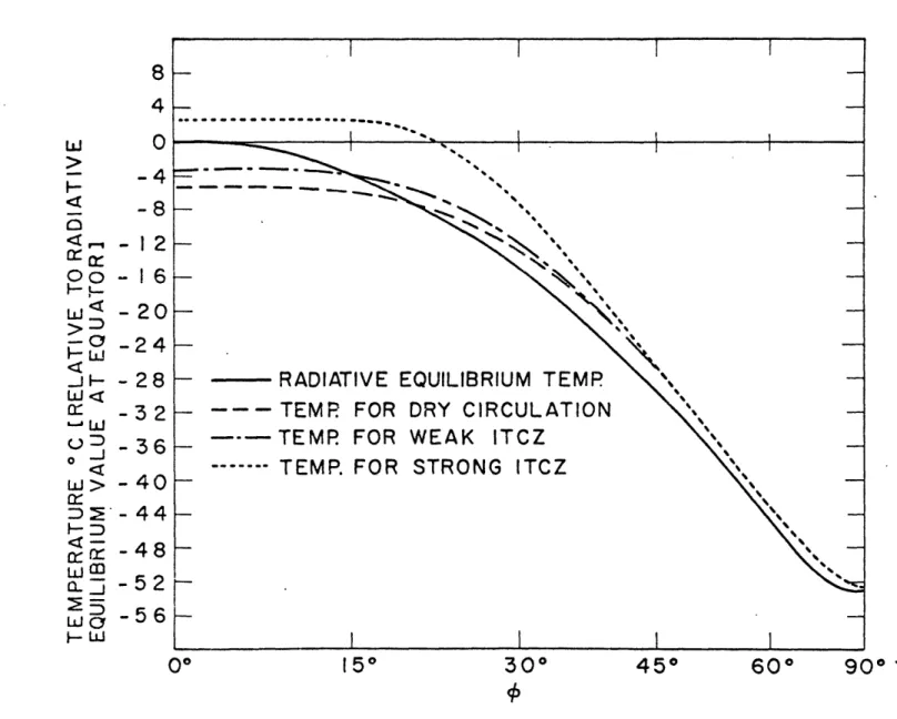
In parameterising the radiative effect, the earth is re-garded as being completely covered by a ocean of fixed temper-ature which varies with latitude according to the formula

T_

T

( )

T,,

3

(2.4.1)

This gives a fair approximation to the observed variation of ocean temperature.

Calculations of the radiative equilibrium temperature profile of the atmosphere by Manabe and M8ller (1961), assuming a fixed temperature at the surface and taking into account the long wave radiation by water vapour, carbon dioxide and ozone and the ab-sorption of solar radiation by these three gases, have shown that the equilibrium profile closely parallels, throughout the tropo-sphere, the dry adiabat from the surface.

This would give, in the present case, a radiative equilibrium temperature at level 2 with latitudinal variation described by

t

-

1 (

(

o)-

(2.4.2)

The greater influence of solar radiation at lower than at higher latitudes, on the average, would lead to a value of Tm in (2.4.2) greater than that in (2.4.1).

A Newtonian law of cooling relative to the radiative equil--ibrium temperature is then assumed for the atmosphere, expressed by

4

C

A

(2.4.3)

A rationale for such a mechanism, based on a linearization of the Boltzmann fourth-power law of heat radiation, has been given by Charney (1968), who arrives at a value of the radiative relaxation constant,A.A, given by

CpPi

a)

4

Z'

3

4

---( " = Boltzmann constant).

The heating of the atmosphere due to the release of latent heat of condensation, which, from the global point of view, oc-curs mainly in the 'hot towers' of the Intertropical Convergence Zone, will be parameterised in terms of the pumping of moisture out of the boundary layer. An elaboration of the Charney and Eliassen (1964) formulation will be used here.

When there is positive pumping of moisture out of the boun-dary layer, all the latent heat will be assumed to be released and distributed uniformly in the vertical, giving rise to a con-densational heating per unit mass

(2.4.6)

For negative pumping, the condensational heating will be zero. It is 'convenient to define a heating coefficient as follows:

-- P -- _(2.4.7)

i.e.

Evaporation from the ocean surface in situ, which supplements the moisture advected by the large-scale flow, will be allowed for by increasing the value of q . To remove the discontinuity in Y in going from a region of positive to one of negative pumping, a multiplicative factor - is employed, defined by

If "rs/SW is large and positive

while if J'L/Dw is large and negative

The boundary layer specific humidity, , is itself a function of latitude. According to Ekman theory, the depth of the boundary layer varies with latitude as I . The air which is in-jected into the base of the 'hot towers' is then taken from higher levels as the equator is approached. Assuming a linear decrease of with height (the actual rhte of decrease is more nearly exponential), it is appropriate to multiply 7 by a factor/r,

where

5

corresponds to some fixed latitude away from the equator. In addition to the latitudinal variation of I due to the change of boundary layer height, there are two other factors whose influence causes to decrease with increasing latitude. In the first place, the static stability ~' increases with latitude and in the second place, is diminished due to decreasing sea surface temperature going to higher latitudes. Both of these effects will

I

be allowed for by multiplying 2 by a factor j; which

is approximately 1 for

4<cf

, and tends to zero for 9p;; . As seen previously, the static stability in the mean and perturbation thermodynamic equations (2.2.16) and (2.3.10) is not allowed to vary with time. The relative effect of the condensational heating term in these equations decreases as the static stability

increases, however, and it is essential to take this into account in some way. This is done in an indirect manner by multiplying by a factor (8),4 O.

The final form of

2

is then

±

SA

It remains to arrive at an expression for the boundary layer pumping,

_(J.

Charney (1968) 1, in his zonally symmetric ITCZ study, used

1. In the reference quoted, Charney did not give the details of the derivation of the expression (2.4.10). His derivation is as follows:

Assuming that the time scale of adjustment in the boundary layer is small in comparison to that of the flow under consideration, the zonal momentum equation for the boundary layer on a sphere may be approximated by

U4t4

C)s

Integration of the above equation and the continuity equation

_+ .0,, (2)

through the boundary layer then gives

+

c

e

0

(4)

,CoS

-where the subscripts "L" denote quantities at the top of the boundary layer, (U) is the weighted average of u in the boundary layer, and

the expression

4

J

(2.4.10)

where

[

(

)

denotes the weighted average through the depth of the boundary layer.]

In this study, where - variations are included, a corres-ponding expression, which reduces to Charney's when all pertur-bation quantities are zero, is used, viz.,

Ie'

I.

(

.1

with

1. Continued

t3 fesT'd is the meridional mass transport in the boundary

layer.

Eliminating FSL&&., the following differential equation in

t3

is obtained:

a'o. q ₍₅₎

where = ^ .

Assuming the first term is small, this equation reduces to In conjunction with (), this leads to the expression (6) In conjunction with (4), this leads to the expression (2.4.10).

Here, it is assumed that

- I

[Results of numerical integrations show that f. and are small terms in the denominator of (2.4.11).]

The expressions for

t

and ? are taken as follows:

62)

p~(~

----

)-(-Y

~

tk

=

ii

fr

Y(W)

(u')

\15

is neglected because of its smallness (verified a posteriori) and because retaining it would give rise to problems in solving the equations, as will be seen later (52.7(e)).

2.5 Spectral Resolution of the Perturbation Equations

The -variation of each perturbation quantity, ! , within the basic period

X

, will be represented by a truncated Fourier series:

where

Fj()

NL

p5

C

i)

(2.5.2)

{U

I

O/.

(2.5.3)

Note: The convention will be used that whenever two subscripted quantities appear within curly brackets, the upper will refer to

even values of the subscript, the lower to odd values.

It is easily seen that the functions F. so defined have the following properties

(a) Zero mean:

(b) Orthonormality:

i.e.

F

"

j"

where

Si

is the Kronecker delta

(c)

32a.

IuF;

FiFjFk = if (i,j,k) are all even and any one of them equals the sum or difference of the other two F.F.Fk if one of (i,j,k) is even, while the other two

are odd, and the even one equals the difference of the other two

FiFF k = - if one of (i,j,k) is even, while the other

two are odd, and the even one equals the sum of the others plus 2

F.F.F. = 0 in all other cases. i k

The quantities _l, 0 ). are expanded to give

3.1

V--Jf

T

-;F 4 Xi(v Fj\

From (2.3.12), (2.3.13), it then follows that

J=)

VA

1 C*r IS /vi (d) (e) (2.5.4) (2.5.5) (2.5.6) (2.5.7)

(2.5.8)

(2.5.9)

where

Similarly for (43 1 1 v .

The non-linear terms in the perturbation equations are also represented by truncated Fourier series:

j!I WO

_-

(

),)

=

r et,

etc& j

\7

d I) JRL

g'Ie FA

(2.5.10)

The interaction coefficients are found by multiplying across by Fj.), taking the mean and using the orthonormality of the functions

F.(4. Hence 1(0'b

C1=

_{_5I?}

=

~2w

~ti~t

fw 5(r,2 £=i =:, e-- ccl Ft F DF Z

Re

j

15-A -FcI C

A~fPFt

_{i - 6A}

(Th()

~

3

c

F,-a C04g

_(2.5.11) S1, [ -

CA

. _

Z]

-a

<"

-I' (4I 'h C,j

trl) Fj.(A

Fe Pj .

₅₎

-ISet

With this representation, the averaged non-linear terms

S

(VyW)

etc., all disappear from the perturbation equations, as can be seen by taking the means of (2.5.10) and using property

(a) of the functions F..

The perturbation frictional terms are likewise resolved: Lateral friction

Internal vertical friction

Vi~

'-7

-A:

~s-(

)F

A)

(2.5.12) Ground friction

J-The perturbation condensational heating term is represented as

S-~$~~t)Flh)

.,(,'(2.5.13)

where

()

_(2.5.14)

Since (?1 t) is a highly non-linear function of the perturbation variables, the coefficients Q are evaluated numerically.

The perturbation vorticity and thermodynamic equations, (2.3.18), (2.3.19) and (2.3.10),

can now be separated into a set of equations for the spectral coef-, by equating the coefficients of F (~).

fThuicients Thus - -

a

1. *13) j -

-

i

ajtI

eijh

(2.5.15) + Ar~S~.

ar.

7%1J

S-VLV

9

+.. .. LI etCf

-4j

_-=*S31

(2.5.16)

Taking the sum and difference of (2.5.15), (2.9. 1 6)

(2.5.17) to eliminate

(2.5.17)

and using

,

i , gives the two prognostic equations

ni:,

~

4b

-ai

'17

Iif~;

-C tj -'1 -i- A V-( I-WI -DU

fj

+

A

T

(Wgj)-JL

r( - L4 Call~ (a. =?+U for

_:

71

(Y+g;

-(2.5.18) -

( (?:I("

_A

V3

Tt p

-

i Z)

_4P

21

+ A W ( Aj A ,-J~~3j~tv

.L'2 .F71

'A)4(Oj

--. , -IL

73

, 1

SCi ^ds

D f

"

aj-AbrgIr

i

CII

c-Examining equations (2.5.15) - (2.5.17), it can be seen that

(1) The lateral friction, ground friction and radiative terms involve no interaction between different spectral components. The vertical internal friction involves interaction between corresponding components at different levels.

(2) The terms involving the mean motion and 06 give interaction between sine and cosine modes of the same wavelength, i.e., they

cause progression of a wave component.

interaction between modes of different wavelength, depending on whether ~35 ~ is non-vanishing. In order that there be any non-linear interaction, J must be greater than 2.

(4) The highly non-linear term : gives interaction between all components, so that no matter what initial conditions are chosen, every component is excited.

Energy Equations

In order to obtain perturbation energy equations,V, (=,)1 is multiplied by C([~.) , V j) F) is multiplied by tI' F), and the products are added and integrated

1- ( )_{OA 641 . Making use of equations (2.5.15) and (2.5.16),}

together with the orthogonality property of the F.s and the boundary contitions

=

0 O j0 (2.5.20)

it is found that

j

(t

1 .

-L9

_

It is to be noted that the contributions from the non-linear terms and from the terms have integrated to zero.

Similarly, on multiplying (2.5.17) by (P~j~Pj ) and integrating, it is found that

(2.5.22)

Again, the contributions from the non-linear terms have integrated to zero.

These perturbation energy equations are consistent with the mean energy equations (2.2.30), (2.2.31).

2.6 The Governing Equations in Dimensionless Form

For convenience in solving the equations and in order to see what dimensionless parameters are important for the motion, the mean and perturbation equations are non-dimensionalized. In

ad-dition, a transformation of the latitudinal co-ordinate is effected by defining

(2.6.1)

A dimensionless time variable, t', and dimensionless dependent

A A A

variables U, W, V, T, j, , ej are defined as follows:

t

aI -UZI V (2.6.2) employ, _(are:L A

Additional dimensionless quantities, which are convenient to employ , are:

I

,A ,A C I C11 G,- I~Caj tlj

e

it

a '

I'

K"

K

(A 'v, _2%. -~V. 174

J

(

) 4.,'-I C3i

OL

=J --

tsJ.

/JL L I - 4 c I I PP ..ft.

C/

'5 !*

CL PA

Kz

=U

tykd~ \Trd1e ,a ven, wc'( Matwnu3)

In all that follows, the prime in t'

Mean Flow Equations

The sum and difference of (2.2.17), (2.2.18) give, on non-dimensionalization

Lt

= -V

[

(k)w

-w

[C'

-vV1

-I--. '

,.LA

-wl

(-LAW)

(2.6.4)

Wt*

-

-V

L

1KFV(JV, V/-f

VLI

'W*f

_{[ 12W1}

(2.6.5)

The dimensionless thermal wind equation, derived from (2.2.19) minus (2.2.20), becomes

(2.6.6)

The thermodynamic equation (2.2.16) becomes

-

(tJ')VAL

*"

t;TT

f&$)Fr3

(2.6.7) is dropped.

+ c rl

I U(U-

W I (Lit -W)

-

itm)

Perturbation Equations

The non-dimensional forms of (2.5.18), (2.5.19) and (2.5.17) can be written A

(

-

A)

(2.6.9) (2.6.10) (2.6.11) where

7,

= - , -__ _ A AA A

- ci -

a

'i

'

L4 VII-I Aj -A -r4.~

~~

U LMt1 ' "t "

R~

A1

(-

;)

S r A A +1- _te A

1-i-( x

'A

'

_(..

I

141

-,A)

.- J. ]

71--7

) +23 K V

17( ; *y P~j 4YI z I%.Y d

4-cV

c 3f L wi

, 1

( (

j

and A

., = value of y at which

4,

and are expressed.

The dimensionless forms of the interaction coefficients, derived from (2.5.11) are A

cli

A

c

₃

_,

A

Y

2

i

- 3j

e:,

&{a -FI

QK

F

F'

(2.6.12)

(

A1

A A f ---4K Ft Fi rk-,

~H)

12

~o~Cr~

i F~ir-t 1r; Fr~ 7- 3

Condensational Heating Term

The non-dimensionalized boundary layer pumping is given by

A

E

I(ra(!

3 (2.6.13) -

att

Fe i F

I

4414 F Fi F.l a~ lr~;I-tfl ~rr~I

,1

.=

0-

_'

U-

+ aj

r

)

4

r 6

.

.. j

63

where

" .(2.6.14)

-

A

T

I.

J=(

In order to non-dimensionalize the condensational heating factor,

, the static stability factor 402 is expressed as follows:

I+i

_,,

_-

_TU)6T

-

.---(2.6.15) Here

Hence

it

( )

where

I -i--

ei

and I o0 - 5 Q)

/

The mean and perturbation condensational heating terms are then

(2.6.18)

(2.6.19)

(2.6.10)

LJ4

2

_{, (zAF()}

Energy Equations

In dimensionless form, the mean and perturbation energy

equations (2.2.30), (2.2.31), (2.5.21) and (2.5.22) can be written

I-(2.6.21)

ZK-f

c c (2.6.16) (2.6.17)

-il

ItG~f~L~u

~ILCI

z~

Cip

T'. hij -~-r

~

A

I

li-C-W

where Ex , , , Ep are, respectively, the mean and per-turbation kinetic and potential energies, given by

F=

f.'

-)u(-wi)[i

E

C L

-

r u+

-~

In

L.-, I

~,"~i~dU~lEb

_t i-(2.6.22) ___

~4

The transformation terms, in dimensionless form, become

J.

4

_[

_-~3

_]

_.

f[ P'f~-.-s:

-~4

~1

[-

'-;,3

{~e

E0

I1

45 L~

IRT)Atl~4

tt

eD~e

I

"at

(2.6.21, cont.)

)~K

Er

(2.6.23)

e~

E i i

b~b ~-r

~lii-i

-d

I

.:A3

J=1

(,^

-

*j)

+ILi( rr

i ~

=-lb'n

tjix E-.C