Dynamic, personalized discrete choice incentive allocation to optimize system performance

Dynamic, Personalized Discrete Choice Incentive

Allocation to Optimize System Performance

by

David A. Sukhin

Submitted to the Department of Electrical Engineering and Computer

Science

in partial fulfillment of the requirements for the degree of

Masters of Science in Computer Science and Engineering

at the

OF1

MASSACHUSETTS INSTITUTE OF TECHNOLOGY

AU

June 2017

LIE

David A. Sukhin, MMXVII. All rights reserved.

The author hereby grants to MIT permission to reproduce and to

distribute publicly paper and electronic copies of this thesis document

in whole or in part in any medium now known or hereafter created.

A uthor ...

3

14

2017

RARIES

ARCHIVES

Signature redacted

Department of Electrical Engineering and Computer Science

May 26, 2017

Certified by...

Signature redacted

Moshe Ben-Akiva

Edmund K. Turner Professor of Civil and Environmental Engineering

Thesis Supervisor

Accepted by ...

Signature redacted

\JA

Christopher J. Terman

Chairman, Masters of Engineering Thesis Committee

Dynamic, Personalized Discrete Choice Incentive Allocation

to Optimize System Performance

by

David A. Sukhin

Submitted to the Department of Electrical Engineering and Computer Science on May 26, 2017, in partial fulfillment of the

requirements for the degree of

Masters of Science in Computer Science and Engineering

Abstract

Incentivization is a powerful way to get independent agents to make choices that drive a system to a desired optimum. Simply offering compensation for making a certain choice is enough to change the behavior of some people. If you incentivize the right choices, you can get closer to your desired choice-dependent goal. Ways to optimize these choices in an environment with many choices and many users is essential for achieving goals for the least cost. I examine how a model that is aware of the utility function of each choice and for each user in a system can optimally allocate incen-tives in real time while considering opportunity cost, personalized incentive response behavior, and maximizing marginal results. This method is useful in systems that have direct and private communication with each user but are limited by having users enter the system at different times. The method must offer a menu of choices and incentives on demand while still considering users that are yet to come. I discuss several solutions and benchmark them on the TRIPOD traffic optimization system which aims to incentivize users to make energy efficient daily commute choices. The final model incorporates user personalized incentives and opportunity cost of each incentive to achieve the optimal incentive allocation on an ad-hoc basis.

Thesis Supervisor: Moshe Ben-Akiva

Acknowledgments

I would like to thank everyone working on the DynaMIT and TRIPOD projects at

MIT, UMass Amherst, and the Singapore-MIT Alliance for Research and Technology (SMART). I would like to give a special thanks to Carlos Azevedo, Ravi Sheshadri, Bilge Atasoy, Hyoshin Park, and Song Gao for their in depth conversations, guidance, and thought-provoking questions and ideas as well as their comments on the final drafts of this report.

Contents

1 An Initial Incentive System 9

1.1 The Goal of the TRIPOD System ... ... 9

1.2 The Token Energy Value System . . . . 10

1.3 Initial Energy Saving Results . . . . 12

1.4 Limitations and Improvements . . . . 12

1.4.1 Simple Ideas to Improve the Simple Method . . . . 13

1.4.2 Larger Limitations of the Impersonal Approach . . . . 15

2 The Optimized Marginal Savings Model 19 2.1 Marginal Token Allocation . . . . 19

2.1.1 Per User Optimization . . . . 19

2.1.2 Opportunity Cost of a Token . . . . 21

2.1.3 Allocating Tokens Optimally Using the MS Curve . . . . 22

2.2 Properties of the Optimized Method . . . . 23

2.2.1 Methods of Calculating the MS Curve . . . . 23

2.2.2 Fully Ad-hoc versus the Benefit of a bit of Waiting . . . . 24

2.2.3 Benefits of Automatic User Recalibration . . . . 25

2.2.4 A Natural Limit on Token Usage . . . . 26

2.2.5 Using the MS to Calculate Token Budgets . . . . 26

3 Simulation Results and Contributions 29 3.1 Experiment Parameter Setup . . . . 29

3.2 Simulation Setup . . . . 32

List of Figures

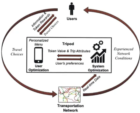
1-1 An overview of the TRIPOD System. Real time information about

traffic is used to measure and predict demand. Users of the TRIPOD app are dynamically incentivized to make more efficient choices by offering them tokens. The number of tokens is optimized using the latest information about the user and the network. The system rewards users if they accept the incentive and follow-through on the optimized

choice. . . . . 10

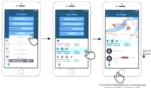
1-2 The TRIPOD trip planner app. Users enter their origin and destination and are presented with route, mode, and departure time choices which

have incentives attached to energy saving options. . . . . 11

1-3 This shows the energy and travel time savings results from a car-only

network at different TRIPOD app user penetration rates (labeled next to each point). At 100% user penetration, the Token Energy Value extension in the DynaMIT simulation engine shows a 17.3% reduction

in travel time and a 16.2% reduction in energy use. . . . . 13

1-4 The post token utility (x-axis) to energy use (y-axis) of a user who is in a hurry or has a high value of time; the tokens have limited effect on the utilities because the user placed higher relative value on their

tim e. . . . . 16

1-5 The post token utility (x-axis) to energy use (y-axis) of a user who

prefers their bike or naturally prefers cheaper and greener forms of transportation; the allocated tokens to the bike option are wasted

2-1 The marginal token response curves for three different types of users with different beta parameters. The "college student" curve peaks early, showing a high impact after just a few tokens, while the token impact on the "wealthy" user happens after a larger token investment. The dotted curve is the MS curve over this population of users and the pink circles represent the optimized token allocations to the "wealthy"

and "college student" users. . . . . 22

3-1 The derived mean and covariance matrix of the betas of the population

colorized by correlation level for easy parsing. . . . . 31

3-2 The results of a Token Energy Value pre-optimization. Using a budget

of 10K tokens, the TokenEnergyValue that achieves the lowest energy in simulation is chosen as the value for the interval. Here, 0.23

To-ken/EU is the best solution. . . . . 32

3-3 Plotted in blue, the top line is the baseline method without tokens. It

used 112,235 EU. Plotted in red just below the top is the Token Energy Value method which used 90,127 EU (a savings of 19.7%) and gave out

10009.6383 tokens to achieve that. Plotted in green at the bottom of

the graph is the new Optimized Marginal Savings model which used only 23,586 EU for the same 2000 users (a 78.9% savings) and gave

Chapter 1

An Initial Incentive System

1.1

The Goal of the TRIPOD System

The TRIPOD system [4, Ben-Akiva, 2015-Present] is based on the simple idea that a reward can be used to incentivize people to make system optimal choices in their

commutes and travel [1], [5], [7],

18].

decrease energy use around a road network [6], [9]. This system works by using real

time information from the road network and by offering users of the TRIPOD system incentives to make choices that are optimal for the network (such as reducing energy usage).

Tokens/rewards are traded for time and convenience in individuals' discrete choice models. This is implemented by offering "tokens" to a user based on the route that they choose to take from a given origin to a given destination. These tokens are meant to incentivize users to choose routes and mode options that use less total energy.

Our goal is to use these tokens (which may be redeemed for prizes, etc. and therefore represent a monetary cost to the issuing system) in the most effective way

possible. I aim to maximize the impact of each token - minimizing our total token

usage while maximizing the resulting energy savings. We must be careful to consider how much value these tokens have to each user so that we neither waste tokens where they are not needed, dilute their value, nor lose out on incentivizing a user to save a large amount of energy at once if we don't give them enough incentive.

Users

Personalized

Menu Tripod

Travel Token Value & Trip Attributes Experienced

Choices Network

Conditions

Users preferences System

User Sse

Optimization Optimization

Transportation

Network

Figure 1-1: An overview of the TRIPOD System. Real time information about traffic is used to measure and predict demand. Users of the TRIPOD app are dynamically incentivized to make more efficient choices by offering them tokens. The number of tokens is optimized using the latest information about the user and the network. The system rewards users if they accept the incentive and follow-through on the optimized choice.

The first half of this first chapter of will describe an initial version of an incentive system that is already showing some promising results. The second half will discuss some of the limitations and flaws of the simple design. Chapter 2 will go on to introduce and formalize a more robust, personalized, and optimized model. Chapter

3 will show a comparison between these systems and discuss the benefits of the more

complete model described in Chapter 2.

1.2

_{The Token Energy Value System}

The first version of this system offers tokens based on the average energy use of all trip alternatives. We implemented this on top of the DynaMIT [2, Ben-Akiva, 20101 short-term traffic simulation, estimation, and prediction engine and applied the token rewards to simulated users' route choices in order to measure the effect on

energy savings. The initial implementation contains three main components: 1. Token Energy Value optimization by minimizing simulated energy use 2. Max token usage budget per a given interval

3. Uniform token allocation based on energy savings over the "average" trip

We can define a Token Energy Value system as TRIPOD (TokenEnergyValue, MaxTokens). The TokenEnergyValue is optimized for the whole system at each inter-val by trying to minimize simulated energy use while using at most MaxTokens. This method implicitly takes into account the allocation strategy, different user choices, and the limit on token disbursement.

tad~ b~ 9

0

0

cetwo 47$Au fox"

A 77-. Scrollwoi~

down

Click on the Dashboard icon to change page and move to the user token wallet

Figure 1-2: The TRIPOD trip planner app. Users enter their origin and destination and are presented with route, mode, and departure time choices which have incentives attached to energy saving options.

When a user visits the system (a mobile trip planning app, Figure 1-2), they enter their origin and destination. The system generates the entire set of route, mode, and departure time options that are possible. For example, a user may take a car or their bike, they may leave now or 15 minutes from now when traffic is expected to be reduced (and thus less idle time/energy use), or they may take different routes (highway/side streets/etc.) which have different expected energy utilization. This is

very similar to how Google Maps allows a user to plan a trip, except with the added benefit of suggesting and pushing users toward energy efficient options rather than offloading that consideration back onto the user [1, Balakrishna, 2016].

After generating all the possible options, the average expected energy usage of that given trip is computed and tokens are allocated to the alternatives that use less than average in a manner proportional to the token energy value as defined by the equation below. A subset of the alternatives that likely appeal most to a user are provided on a shortened menu and the user chooses from them. Hopefully, they choose an alternative with tokens that saves some energy in expectation.

k, = _{max (0,TokenEnergyValue- (average(E(T)) - E(Ti)))}

1.3

Initial Energy Saving Results

Using this easy to implement method, I built and extension to the DynaMIT system to measure both the energy savings and travel time savings that result from incentivizing users to change their route or departure times on a car-only network. Figure 1-3 shows a scatter plot of the average realized energy and travel time savings on the simulated road network at different penetration rates of TRIPOD app users. Not surprisingly, we achieve the biggest energy and travel time reductions if we are able to offer incentives to 100% of the users on the network. At 100% penetration, we are able to achieve a 17.3% reduction in travel time and a 16.2% reduction in energy use.

1.4

Limitations and Improvements

The following sections describe some limitations and potential improvements to the Token Energy Value system which can make the incentive allocation more person-alized and robust. Chapter 2 discusses in much more detail a new method that is better suited to distribute tokens in a more personalized and system optimal way.

S 18% -16Yo 100% 16% - --- - -- - - 86 % 14% --72% 12% - - - -10% -- --- - - --%40% 32% W _6% 20% e 25% 4%- -- ---- - -2% 0% - --- --0% 2% 4% 6% 8% 10% 12% 14% 16% 18% 20%

Travel Time Reduction

Figure 1-3: This shows the energy and travel time savings results from a car-only net-work at different TRIPOD app user penetration rates (labeled next to each point). At 100% user penetration, the Token Energy Value extension in the DynaMIT simu-lation engine shows a 17.3% reduction in travel time and a 16.2% reduction in energy use.

1.4.1

Simple Ideas to Improve the Simple Method

Immediately, we can consider ways to improve our estimate of how many tokens to allocate to each trip choice alternative. We can better quantify the choice users are really making by understanding what trip route they would have chosen before incentives or knowledge of how much energy their choice uses. This can be done either

by simulation on the back-end or by changing the app menu flow to (1) select a route

and then (2) see alternatives with incentives. A better understanding of what we are trying to incentivize away from gives us a clearer picture of how much energy we

stand to save (instead of using the nebulous "average") and what impact on the user

we are directly proposing, and therefore how much we should be compensating them. This implicitly solves the issue of what the baseline "alternative" is which may be a route that is not proposed on the shortened menu at all. By simulating or asking the user to select a baseline trip that they will take without any incentives, we minimize our uncertainty (of expected energy use) and provide ourselves a baseline option that a user is willing to pick without any token usage.

Eventually this even affords us the flexibility to gently whittle down the incentives in the long term (on a per user basis) and allow their new route choices to become

habit instead of a token earning endeavor forever.

Additionally, savings over the "average" trip suffers from a bad distributional

assumption - suppose there are four possible alternatives - two with very high energy

use and a two with very low energy use. Savings over the "average" trip will only allocate half of the difference in energy as tokens between the two extreme options even though the user would be saving the full difference because there is no "average" trip they could have taken. Not only is including the incentivized alternative itself in the calculation of "average" skewing the token reward downward, but incentivizing for only energy savings ignores how different users respond to the token and different trip proposals.

From these observations, I propose some simple changes that we can make (in order) before we move on to a more complete overhaul that puts more emphasis on user specific behaviors.

1. Remove the incentivized trip from the calculation of average energy usage... we

should only be considering the average alternative trips energy usage.

2. Use a more distributionally robust average method like median or the geometric mean to calculate the expected alternative energy use.

3. Weight the average energy usage of these alternative trips by the probability a

user will select them as alternatives.

4. Simulate or ask what a user's most probable baseline choice will be and allocate incentives based off of that instead of a weighted average of alternatives.

5. Use tokens to affect the probability (of trip selection) weighted expected energy

use to be a certain percentage above the baseline probability weighted expected energy use. This method will ensure that only energy saving trips are incen-tivized and that we are properly considering how useful a given token is applied to each given trip (i.e. some trips don't impose a large inconvenience but save a lot more energy therefore a token is better used on a such trips to increase

their probability of selection with fewer tokens but more energy savings). This allows us to reduce the token usage when it is easier to incentivize a given user.

1.4.2

Larger Limitations of the Impersonal Approach

While we already see some great initial energy saving results in Section 1.3 and we can suggest some simple improvements, we must also recognize that there is some considerable value being left on the table and that we are not necessarily incentivizing the right metric.

We can notice that the only parameter being "optimized" in the Token Energy Framework is the energy value of the token. However, this value is heavily dependent on the arbitrary token budget constraint (MaxTokens) we set. If we arbitrarily set a max budget too low, our initial system optimization will simply set the token energy value low enough that it can incentivize a subset of users with low enough token energy value and therefore a high enough number of tokens. Thus tokens will be spent rather greedily and far too early in each interval without regard to the users that may come later. By relying on a fixed budget to limit token allocation rather than considering the opportunity cost of each token as a way to ration use, we may be spending tokens in the wrong place and at the wrong time.

In the Token Energy Value system, some users may get more tokens than they need to comply with our trip proposals, while others may need a bigger push to take a trip that saves a lot of energy at once. We can also recognize that allocating tokens based on the energy savings over an "average" trip sometimes does not adequately balance the changes in travel time or convenience for a user. Therefore, the tokens should not be exchanged for "energy" directly but for the impact that changing to a different trip proposal has on a user because they are the agent making the primary decision that causes the energy savings. By attempting to pay a user for the energy they save, we ignore the dynamics of how travel time and convenience play into the decision they are making.

Below are two illustrative examples. Figure 1-4 is a user that has a high value of

flexible schedule and that prefers to bike.

Figure 1-4: The post token utility (x-axis) to energy use (y-(x-axis) of a user who is in a hurry or has a high value of time; the tokens have limited effect on the utilities because the user placed higher relative value on their time.

Figure 1-5: The post token utility (x-axis) to energy use (y-(x-axis) of a user who prefers their bike or naturally prefers cheaper and greener forms of trans-portation; the allocated tokens to the bike option are wasted because that was the most likely choice already.

In both cases, the tokens we allocate have little to no effect. For the first user who is in a hurry, the tokens allocated based on the energy savings over the average option were not enough to make him consider to take a mode of transport other than his car. For the bike rider, they will happily collect the tokens, but would have likely used their bike anyway. That just means we have wasted tokens that could have been better used elsewhere.

From the problems I discussed above, we clearly see that we must begin to con-sider (1) how many tokens to allocate per alternative based on an individual user's preferences/betas and (2) how many tokens we should allocate to a user (based on the tokens' impact for that user) as opposed to saving the tokens to allocate later.

I do this by considering the impact different alternative choices have on important

metrics to users such as time and convenience while allocating tokens. Thus, tokens will be distributed where they have the most impact both at the user level and at the system level.

If we incentivize users for their time and choices, we gain the ability to incentivize

different users differently. The price to sway a given user may be different from

100 60-40 20 -20 -12 -11 -10 -9 -8 -7 10 80 60 40 20 0. -20~_-10 -9 -8 -7 -6 -5 -4 -3 -2 -1 5

another user and we can take advantage of this with price discrimination strategies as we learn about each user's preferences and prices and the probability another user (or set of users) may appear on our network that may be swayed more easily for the same (or more) energy savings later on.

Chapter 2

The Optimized Marginal Savings

Model

2.1

Marginal Token Allocation

The proposed model, the Marginal Savings Model, will consider how to allocate tokens most effectively among a user's trip options and will also consider the opportunity cost of using the tokens allocated to a user later on.

2.1.1 Per User Optimization

We began to discuss that it is important to allocate tokens to the trips where they provide the most impact on expected energy savings. The following optimization setup minimizes the maximum number of tokens allocated to any of the trip options

while making sure the expected energy usage is some multiple n < 1.0 of the baseline

expected energy usage. The probability a given trip is selected is based on a Discrete Choice Model which uses a logit to estimate the probability of selection from the utility of each choice. [3, Ben-Akiva, Discrete Choice, 19851

k =argminE Pr(T,(k)) -E(T) < nr- ( Pr(Ti(O))-E(T. )

max(k) T _/

T is the set of all trip alternatives

Ti(ki) is the alternative with k tokens allocated to it Ti(0) is therefore the baseline without any tokens E(T) is the energy use of alternative trip T

Pr(T) is the probability that alternative is taken: exp(,3Ti)

E exp (/Ti) k is the vector of token allocations for all trips in T

n is a free parameter that we can set to achieve a given energy savings level

We are able to minimize for max(k) because at most one of the alternatives will be chosen and thus the cost of the trip is at most the maximum number of tokens allocated to any given route choice. That does in fact mean that we can add tokens (without penalty) to all trips up to max(k). When we have a linear utility function, this actually means that we will either fully allocate max(k) tokens to a trip, or none at all because allocating extra tokens only improves the probability of selection of these energy saving trips. It is possible to design a token utility function where this is not true, where it makes more sense to use the number of tokens allocated to an option as a signal for how likely it is to be chosen such that it saves energy over the baseline, but if it is too valuable, may cannibalize the more impressive savings of another option.

The token array k can be constrained to be integers so we can perform integer optimization on this problem. The substantial advantage of this formulation is that each trip choice changes in probability at a different rate and tokens will continue to be allocated to the best energy saving trip that can be increased in probability the quickest. This continues until a token has more marginal value on another energy saving trip. Tokens are not allocated greedily to a single trip but rather to the trips where they have the most impact. The overall expected energy usage is set to a target value with the smallest number of tokens needed.

Moreover, this formulation can be adjusted as needed, The constraint can be changed from a minimum desired energy savings, to a maximum number of tokens used and we can instead minimize the energy use. Regardless of how it is structured, this equation represents an optimized allocation of tokens on a per user basis by considering the utility of each route choice.

2.1.2

Opportunity Cost of a Token

Now that we can optimize how tokens are used within a given user, we can consider how much energy we want to save (either in percentage or absolute terms) such that the tokens we use are not better used later on. This can be captured in a simple probabilistic average that accounts for user and trip heterogeneity and the benefit of high energy saving trips, while minimizing the tokens on a per user basis. We can bootstrap the per user optimization described above to calculate the expected cost of a token and only use it on a user if its benefit meets or exceeds the expected cost of not being able to use that token later.

The expected energy savings of a given set of trip options with optimized tokens should (in expectation) be greater than or equal to the expected energy savings of a randomly drawn user (or set of users) using the same number of tokens or fewer.

We can define this opportunity cost of a token as the average marginal energy savings up through k tokens (MSk). We don't only consider the marginal value of the first token but the average marginal value of an investment of up to k tokens. This allows us to consider users that require a few tokens of investment before we can reap above-average energy saving results from them. See Figure 2-1 for an example.

_( E(UT(-1)) _{- E(UT(n)))}

MSk _{Pr(U) - Pr(Ur) -E}

k

U T

Here, U refers to a user and Pr(U) refers to the probability of seeing that user on the network. Pr(UT) is similarly the probability that a given user takes a given trip.

This equation simply computes the marginal savings E(UT(n_1)) - E(UT(s)) at each

through k so that we are considering not only the expected value of the k-th token

but also the expected marginal savings of investment of the previous k - 1 tokens

that are invested into a user. The MS curve is pictured in dashed blue in Figure 2-1.

Marginal Token Savings by User

25 - ---

-120___

- Wealthy & Time Sensitive

- College Student

- Price Sensitive Biker

I - - - (Average MS up to k)

0

-0 2 4 6 8 101214161820222426283032 34363840424446

Tokens

Figure 2-1: The marginal token response curves for three different types of users with different beta parameters. The "college student" curve peaks early, showing a high impact after just a few tokens, while the token impact on the "wealthy" user happens after a larger token investment. The dotted curve is the MS curve over this population of users and the pink circles represent the optimized token allocations to the "wealthy" and "college student" users.

2.1.3

Allocating Tokens Optimally Using the MS Curve

The MSk curve is the opportunity cost of an investment of up to k tokens into a given user. Therefore, the intersection of the MS curve with the marginal benefit of the k-th token per user curves (marked by circles in Figure 2-1), are the optimized token allocation per user.

We need to observe two rules when allocating tokens to users. (1) We want the marginal savings of the k-th token to meet or exceed the MSk value, and (2) we want the total energy savings of the k tokens to a user (the integral of the user marginal curve above) to be greater than or equal to the total expected energy savings with k tokens on the population. We define this as the TSk curve.

TSk = Pr(U) - Pr(U) -E(UrTe))

U T

This simply calculates the expected energy savings with k tokens optimized using the optimized per-user token allocation method. The energy savings of a user's trip with k tokens must be greater than or at least equal to the expected energy use of an average user's trip using at most k tokens. This allows us to amortize initial low value tokens with higher marginal savings later on. This is most clearly visible for the "wealthy" user in Figure 2-1.

This is the same as saying that the optimized energy use of this trip is less than or equal to the energy use of an average optimized trip using the same number of tokens or fewer. This sets a nice limit on how we use tokens to save at least a certain amount of energy; if we cannot save that amount for a certain number of tokens used, it is not worth spending tokens on this trip because (in expectation) another, better user will come along later. Therefore, instead of a token budget (MaxTokens), we control our use of tokens by considering their expected future value.

These two checks over our distribution of other potential users and trips sets an implicit limit on how many tokens can be allocated to a particular user given that there may be other users that place more value on the token that may appear on the network and cause the same or better expected energy savings at a smaller cost to

us.

2.2

Properties of the Optimized Method

2.2.1

Methods of Calculating the MS Curve

The MS curve requires us to have an estimate of the users we expect to see in the future on our network. The better our estimate of the users we expect to see, the more representative our MS curve becomes of our future value (opportunity cost) of our tokens.

users that it expects to see in the next 3 intervals. This can be used directly to compute the MS curve dynamically while running our system. Since we have already have a sample from the distribution of users 3 intervals forward, we just need to take the simple average of all users marginal expected savings at each token level

(by optimizing each user locally) to get the global average marginal expected savings.

This is a very quick computation and can be done "online" (in real-time) as the traffic prediction system is running. This keeps our MS curve fresh and representative of what types of users we expect to see on our network at a given time.

If we want to be more analytical, we can leverage the actual user beta, and trip

distributions and compute an analytical and/or large random sample size sample of the whole population and keep the MS curve as a static parameter (updated infrequently). The MS curve needs to only be calculated once over a reasonable sample of users and corresponding trips for a reasonable subspace of integer k. Using the simulated users gives us some implicit time dependence (as long as there is implicit time dependence in the empirical simulated users). However leaving this relationship time independent perhaps allows us to consider a more indefinite time horizon that tokens will be better spent on a different trip.

The MS curve need not be a single value at each k. Instead, because we are taking an average over several dimensions, we can consider the MS value at k to be distribution. If we want to relax our token allocation criteria and be more liberal, we can move our token allocation MS percentile to 30th instead of the implicit 50th. We should certainly keep in mind that the average (the 50th percentile) is the optimal allocation in expectation, but it might make sense to be a little more generous when our budget exceeds our more conservative usage. This gives us a nice parameter to tweak to control the token usage speed.

2.2.2

Fully

Ad-hoc versus the Benefit of a bit of Waiting

When we allocate tokens in a fully ad-hoc manner, we rely on our understanding of the expected future value of a token in the future to other future users that may appear on our network. This uncertainty about future users is the only constraint

to our problem that prevents us from simply running an optimization to allocate tokens among every user we expect to see (because we don't really know who we expect to see). However, we can recapture some of this uncertainty and therefore recapture some value that we lose by using an estimate of future users instead of a

true knowledge of who we will see next.

By relaxing the requirement to respond to requests for token allocations

imme-diately, and instead waiting, perhaps 2-3 seconds (or whatever amount of time is

reasonable), we can run a full optimization over users and allocate tokens purely based on the per user marginal expected savings curves. This would allow us to capture the value of some smaller benefit users that otherwise fell below the MS curve, such as the "biker" in Figure 4. We can see quite easily from the figure that

the marginal savings of the first two tokens of the "biker" user actually exceed the

savings of the last token of the other two users, despite falling below the MS curve.

If we knew with certainty that we would see all 3 users, we could conduct a rolling

global optimization (still using the MS curve as a guideline). This lets us capture more of this value by simply waiting and collecting more concrete information about what users are coming next.

2.2.3

Benefits of Automatic User Recalibration

As users interact with our system, we have the ability to continuously learn more

about their utility functions (beta parameters). This in turn allows us to produce better estimates of our MS curve and allocate tokens better on the user and system

level. This means that if a user commonly takes a certain trip daily (with a small incentive), the Marginal Savings Model will naturally attempt to reduce the number of tokens needed to continue this behavior. If the user accepts this smaller incentive, the process will continue and discover the minimum price needed to incentivize this user until they begin rejecting our lower incentive proposals (at this point the system

will self-correct).

The by using the latest estimate of users' utility functions, the Marginal Savings Model is able to do some natural price discovery and learn about the user in a

closed-loop way. As we push a user toward certain behaviors, we must consider that we are helping to form a new habit for a user and that our tokens are not simply a cost but rather an investment into a long term habit of energy saving choices. As a user gets more accustomed to a path that we incentivize them toward, the number

of tokens that are required to maintain this behavior naturally decreases - this will

be automatically captured in our continuously recalibrated utility function estimates. This makes this self-adjusting nature a very powerful mechanism to dynamically reduce our cost and help us form habits for our users rather than continually pay them to make certain choices.

2.2.4

A Natural Limit on Token Usage

One of the major benefits of the Marginal Savings Model is that the opportunity cost of a token is built in as we aim to maximize the impact of our incentives. This means that we no longer have to set an arbitrary MaxTokens parameter. Instead our model

limits the number of tokens used by being frugal - by considering the potential benefit

of a token later on versus using it on a user that is immediately available. Moreover, the marginal benefit of tokens is typically higher at lower token investments as we see a diminishing return after some incentive level in most users. This means that the system will also not over allocate tokens to any one particular user and will continue to save them for other users that will come later.

2.2.5

Using the MS to Calculate Token Budgets

In addition to allowing us to allocate tokens to users confidently in an ad-hoc way while still considering the future value, we can use the MS curve to calculate what our total budget should be a priori such that we get the biggest impact per token. As mentioned at the end of Section 2.2.1, this value is simply informative and shows us how to get the most value for our investment but may not correspond with how many tokens we actually have to give out to achieve our total target energy savings. This computation can be done in an ad-hoc way (basically running the full Marginal

Token Allocation strategy that I describe) to get the optimized value, or more accu-rately by actually simulating/predicting all the users that will appear on the network and conducting a global optimization at each possible token count, allocating tokens optimally on a per user basis and among users. This allows us to create a single optimized population average marginal token value that we can similarly compare against the same MS curve in order to understand how many tokens should be al-located to our system as a whole. This may become useful if we have to allocate budgets optionally between multiple cities, for example.

Chapter 3

Simulation Results and Contributions

3.1

Experiment Parameter Setup

In order to measure the effect of the new method compared to the old method and the baseline (no tokens), the following experiment was setup outside of DynaMIT.

A random set of 2000 users was generated and picked one of six simple trip options.

These trips included two routes in a car, an Uber, a train/subway public transit, a bus public transit, and a bike trip. The parameters of these trips (shown at the end of this section) are indicative of a choice a user might have to make during their morning compute in a metropolitan area.

Users were generated from a random distribution with means and a covariance matrix between the betas. For this experiment, the nine beta dimensions were:

" Time e Train 9 Taxi

" Cost e Bike o Miles

" Bus * Car * Tokens

The means and the covariance matrix were derived from a weighted subsample of a few hand designed representative users. Six distinct (extreme) user types were created by hand and weighted to indicate how representative they were of users in the population. The mean and covariance coefficients were easily calculated from

this subsample, the mean by taking the mean of each beta across the subsample of

users and the covariance as the UTU matrix product. This allows us to generalize

these five kinds of extreme users to all the types of users in between while still being representative of how the beta (like for example and time, cost, and token betas) covary. The weightings and betas for the sample users as well as a simple description of their user type is detailed in the table below.

U Q N H O 0 H 0 Description

-0.3 -0.1 -0.2 -0.15 -0.4 0.1 0.2 -0.4 0.3 2/10 Young professional

who values time

and has a modest amount of money

-0.2 -0.5 -0.1 -0.1 0.1 0.1 0.3 -0.2 0.9 4/10 A college student

that is more flexi-ble with time and distance if it means

saving money

-0.1 -0.8 -0.1 0.2 0.3 0.2 0.1 -0.6 0.8 2/10 Particularly

en-vironmentally conscious user who prefers their bike and puts less value on their time

-0.9 -0.1 -0.9 -0.7 -1 0.6 0.5 -0.6 0.1 1/10 Very wealthy user

who needs conve-nience and speed and is not very con-scious about cost and tokens

0.3 -0.9 -0.4 -0.2 -0.3 0.6 -0.1 0.1 0.9 1/10 An Uber driver who

makes a small living

by driving and likes

to earn tokens while

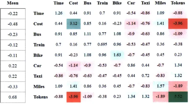
The derived statistics that are used to simulate the population are below: Mean -0.22 -0.48 -0.23 -0.12 -0.11 0.22 0.22 -0.33 0.68 Time Cost Bus Train Bike Car Taxi Miles Tokens Time 1.26 0.44 0.91 0.7 0.91 -0.54 -0.86 1.09 -0.88 Cost 0.44 3.12 0.85 0.16 -0.23 -1.14 -0.76 1.41 -3.96 Bus 0.91 0.85 1.11 0.77 1.08 -0.9 .0.63 0.86 -1.09 Train 0.7 0.16 0.77 0.695 0.96 -0.53 -0.47 0.36 -0.38 Bike 0.91 -0.23 1.08 0.96 1.63 -0.7 -0.45 0.45 0.23 Car -0.54 -1.14 -0.9 -0.53 -0.7 0.86 0.44 -0.7 1.34 Taxi -0.86 -0.76 -0.63 -0.47 -0.45 0.44 0.72 -0.83 1.32 Miles 1.09 1.41 0.86 0.36 0.45 -0.7 -0.83 1.57 -1.89 Tokens -0.88 -3.96 -1.09 -0.38 0.23 1.34 1.32 -1.89 5.52

Figure 3-1: The derived mean and covariance matrix of the betas of the population colorized by correlation level for easy parsing.

Users were generated randomly by selecting from this distribution. Each user's randomly selected betas were then used to weight a choice between six different trip options. These options are shown in the table below.

Q)

e.

S0 EEnergy Use Description

15 4 0 0 0 1 0 4 100 Car Route 2 22 5 0 0 0 1 0 5 87 Car Route 1 27 5 0 0 0 0 1 5 69 Uber 25 4 0 1 0 0 0 7 11 Train 28 2 1 0 0 0 0 5 9 Bus 37 0 0 0 1 0 0 3 1 Bike

3.2

Simulation Setup

Now, that we have some statistics on our population, we can set up three experiments: The baseline with no tokens, token energy value model, and, our optimized marginal savings model. The baseline case is simple, 2000 users are randomly generated (seed 2) and using their utilities for each of the route choices, routes are chosen randomly (weighted by the probability derived from the utility) and an energy use baseline is computed without adding any incentives into the network.

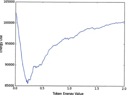
The Token Energy Value model and our new Marginal Savings model require some optimization work upfront. In order to choose an optimized token energy value, we can first choose a different set of 2000 users (from the same population parameters) (seed 1) and optimize the token energy value by doing a simple linear search at a token limit 10K tokens. The result of this initial search is shown in Figure 3-2 showing an optimized token energy value of 0.23.

105000 100000 L 95000 C 90000-850001 0.0 0.5 1.0 1.5 2.0

Token Energy Value

Figure 3-2: The results of a Token Energy Value pre-optimization. Using a budget of 10K tokens, the TokenEnergyValue that achieves the lowest energy in simulation is chosen as the value for the interval. Here, 0.23 Token/EU is the best solution.

We can use this optimized value to compare the Token Energy Value method to the baseline by selecting the same 2000 users (seed 2) and checking the total energy

and token usage.

The same pre-optimization step is done for our new model. I precompute the MS and TS curves from 2000 users of (seed 1) and use these curves to compute the best token allocations on seed 2. The following code snippet describes the exact method for allocating tokens used for this simulation.

def makenewTokenAllocator(ms,ts):

def tokenAllocationNew(user, trips):

u-edist = getEnergyDist(user, trips, t=len(ms))

ums = [0] + [k for k in uedist[:-1]-u_'edist[1:]] for k in xrange(len(rns)-1,-1,-1): #backwards

if (u-edist [0] -u-edist [k] >= ts [k]) and (ums [k] >= ms [k]):

return usertriptokens(user, k, trips)

return [0]*1en(trips) return tokenAllocationNew

Here, getEnergyDist computes the optimized energy use of the user at every token level. Then, ums is the user-specific marginal energy savings curve of each token. We then iterate and check for the highest token value that both exceeds the average total energy savings (the TS curve) and the average marginal energy savings through that token level (the MS curve). Finally, user.triptokens returns the array of tokens corresponding to each trip using a maximum of k tokens.

By optimizing on the initial set of 2000 users (seed 1) for both the token energy

value and the new optimized method, we can perform a more realistic out of sample test on a new set of 2000 users (seed 2). Figure 3-3 shows the CDF of energy use by user of the three models. There is a startling difference between the three methods.

120000

100000

S80000

S8000 No Tokens

W 60000

U

C W Optimized Model 40000-20000 0 500 1000 1500 2000 User #

Figure 3-3: Plotted in blue, the top line is the baseline method without tokens. It used 112,235 EU. Plotted in red just below the top is the Token Energy Value method which used 90,127 EU (a savings of 19.7%) and gave out 10009.6383 tokens to achieve that. Plotted in green at the bottom of the graph is the new Optimized Marginal Savings model which used only 23,586 EU for the same 2000 users (a 78.9% savings) and gave out just 10860 tokens.

The baseline method in blue used 112,235 EU and of course no tokens. The red line, shows the token energy method which uses 90,127 EU and just slightly exceeds its limit using 10009.6383 tokens. That's a 19.7% energy savings over the baseline and a realized energy savings per token of 2.2 EU. However, the green line shows the savings of the new optimized model. For the same 2000 users, we only use 23,586 EU and spend only marginally more tokens (10860). This is an impressive energy savings of 78.9% and nearly a 4 times increase in realized energy savings per token of 8.16

EU. This shows the huge contribution of our new model: we improve both the impact

3.3

Contributions

The goal of this thesis was to drastically improve our capability to incentivize users toward system optimal choices using information about their personalized preferences and utility functions and the distribution of users we expect to see in our system. This was achieved by framing our problem as an ROI (return on investment) maximiza-tion as opposed to simply a target variable (energy use) minimizamaximiza-tion. This allowed us to consider and leverage user preferences and offer incentives where (and only where) they will have the most impact. Token use is minimized and token impact is maximized to achieve the highest ROI.

In the Marginal Savings Model, high value users are captured for minimum cost using price discrimination and cost minimization. Instead of a TokenEnergyValue that sets an exact value for how many tokens to give each user, the MS curve offers a population specific minimum guideline and allows us to capture more value from each user whenever possible. Moreover, the MS curve dynamically adjusts with the number of tokens invested to allow us to explore the possibility of larger investments into certain users that can have a huge positive impact. After calculating the MS curve for our population, incentive allocation is fast and there is no need to contin-ually re-optimize our parameters as the Token Energy Value method needed to do. Additionally, the model is self-correcting as we can continually use the information we get from users' decisions to reestimate their beta parameters and thus re-optimize how much we need to incentivize each user.

In summary, I:

" Formulated a method to optimize the use of each token at the user level by

minimizing token use for a given target energy savings

" Optimized the use of each token at the system level by considering the oppor-tunity cost of each marginal token

" Minimized incentive usage while maximizing incentive impact

Bibliography

[1] Balakrishna, R., Ben-Akiva, M., Bottom, J. and Gao, S., (2013). "Information

Impacts on Traveler Behavior and Network Performance: State of Knowledge and Future Directions". In: Ukkusuri, S. and Ozbay, K. (ed.) Advances in Dynamic Network Modeling in Complex Transportation Systems. Springer. pp. 193-224.

[2] Ben-Akiva, M., Koutsopoulos, H.N., Antoniou, C. and Balakrishna, R., 2010. "Traffic simulation with DynaMIT". In: Fundamentals of traffic simulation (pp.

363-398). Springer New York.

[3] Ben-Akiva M., Lerman S., (1985). Discrete Choice Analysis, The MIT Press,

Cambridge Massachusetts.

141

Sus-tainable Travel Incentives with Prediction, Optimization and Personalization". Ongoing Project/Working Paper: https://its.mit.edu/tripod-sustainable-travel-incentives-prediction-optimization-and-personalization

[51 Ettema, D., Knockaert, J. and Verhoef, E., (2010). "Using incentives as

traf-fic management tool: empirical results of the 'peak avoidance' experiment". In: Transportation Letters: The International Journal of Transportation Research

2:39-51.

[61 Gupta, S., Seshadri, R., Atasoy, B., et al., (2016). "Real Time Optimization of

Network Control Strategies in DynaMIT2.0" In: Transportation Research Board 95th Annual Meeting.

[7] Haq, G., Whitelegg, J., Cinderby S., Owen A., (2008). "The use of personalised

social marketing to foster voluntary behavioral change for sustainable travel and lifestyles", In: Local Environment, 13, pp. 549-569.

[8] Lee, C., Winters, P., Pino, J., Schultz, D., (2013). "Improving the Cost

Effec-tiveness of Financial Incentives in Managing Travel Demand Management". In: Project BDK85977-41, FDOT. USF Center for Urban Transportation Research.

[9] Lu, Y., Seshadri, R., Pereira, F., et al., (2015). "DynaMIT2.0: Architecture

De-sign and Preliminary Results on Real-Time Data Fusion for Traffic Prediction and Crisis Management". In: 18th International IEEE Conference on Intelligent Transportation Systems.