Calculation of ozone line shifting induced by N2 and O2 pressure

HAL Id: hal-00519624

https://hal.archives-ouvertes.fr/hal-00519624

Submitted on 21 Sep 2010

HAL is a multi-disciplinary open access

archive for the deposit and dissemination of sci-entific research documents, whether they are pub-lished or not. The documents may come from teaching and research institutions in France or abroad, or from public or private research centers.

L’archive ouverte pluridisciplinaire HAL, est destinée au dépôt et à la diffusion de documents scientifiques de niveau recherche, publiés ou non, émanant des établissements d’enseignement et de recherche français ou étrangers, des laboratoires publics ou privés.

pressure

Nina Nikolaevna Lavrentieva, Anna Sergeevna Osipova, Jeanna Buldyreva

To cite this version:

Nina Nikolaevna Lavrentieva, Anna Sergeevna Osipova, Jeanna Buldyreva. Calculation of ozone line shifting induced by N2 and O2 pressure. Molecular Physics, Taylor & Francis, 2009, 107 (19), pp.2045-2051. �10.1080/00268970903136639�. �hal-00519624�

For Peer Review Only

Calculation of ozone line shifting induced by N2 and O2 pressure

Journal: Molecular Physics Manuscript ID: TMPH-2009-0156.R1 Manuscript Type: Full Paper

Date Submitted by the

Author: 01-Jun-2009

Complete List of Authors: Lavrentieva, Nina; Institute of Atmospheric Optics Osipova, Anna; Tomsk State University

Buldyreva, Jeanna; Université de Franche Comté, UTINAM

Keywords: ozone, line shift, semiempirical calculation, polarizability in excited vibrational state, temperature exponent

For Peer Review Only

Calculations of ozone line shifting induced by N

2

and O

2

pressure

N. Lavrentieva a, A. Osipova b and J. Buldyreva c*

*

Corresponding author ; Phone: +33 (0)3 81 66 63 60; FAX: +33 (0)3 81 66 64 75; Electronic address : jeanna.buldyreva@univ-fcomte.fr

a

Institute of Atmospheric Optics, 1 ave Akademicheskii, 634055 Tomsk, Russia

b

Tomsk State University, 36 ave Lenina, 634050, Tomsk, Russia

c

Institut UTINAM, UMR CNRS 6213, Université de Franche-Comté, 16 route de Gray, 25030 Besançon cedex, France

1 2 3 4 5 6 7 8 9 10 11 12 13 14 15 16 17 18 19 20 21 22 23 24 25 26 27 28 29 30 31 32 33 34 35 36 37 38 39 40 41 42 43 44 45 46 47 48 49 50 51 52 53 54 55 56 57 58 59 60

For Peer Review Only

Abstract

Ozone line shifts by nitrogen and oxygen pressure are computed for the ν1+ν3, 2ν1 and

2ν3 bands of the 5µm spectral region by a semiempirical approach. The calculated values

agree with measurements better than 0.001 cm-1atm-1 for 98% of O3-N2 lines and 87% of

O3-O2 lines. In contrast with the water molecule case, the polarization components of the

interaction potential are shown to contribute to the line shift more efficiently than the electrostatic interactions. As intermediate results, the mean dipole polarizability and the components of the polarizability tensor for the vibrational states (101), (200), and (002) of ozone molecule are determined by least-squares fitting of theoretical shifts to some experimental values. The temperature exponents for the ν1+ν3 band lines are also estimated.

Keywords: ozone, line shift, semiempirical calculation, polarizability in excited vibrational state, temperature exponent

1 2 3 4 5 6 7 8 9 10 11 12 13 14 15 16 17 18 19 20 21 22 23 24 25 26 27 28 29 30 31 32 33 34 35 36 37 38 39 40 41 42 43 44 45 46 47 48 49 50 51 52 53 54 55 56 57 58 59 60

For Peer Review Only

I. Introduction

Among the minor constituents of the Earth’s atmosphere ozone receives a particular attention of scientists due to its double role of protector and pollutant: whereas the stratospheric ozone layer protects the humans, animals and vegetation from the harmful ultraviolet radiation of the Sun, the excessive concentration of ozone in the troposphere is qualified as pollution because of its toxic effects for respiration. Precise measurements of vertical ozone concentration profiles are therefore of crucial importance for health protection services and scientific community interested in comprehension and global modelling of the terrestrial atmosphere.

The probing of atmospheric species is principally realized by non intrusive spectroscopic techniques in the infrared, microwave and millimeter domains. For ozone, the spectral regions of 5 µm and 10 µm are of particular interest since they correspond simultaneously to its most intense absorption bands and to “atmospheric windows” free of water vapour absorption. Reliable inversion of the recorded spectra requires a precise knowledge of ozone spectral line shape parameters (including its main isotopic species) in a wide temperature range and in different vibrational bands.

While the ozone line broadening has been quite intensively studied both experimentally and theoretically, its line shifting data remain quite sparse. Only some measurements were made by Smith et al. [1-4], Barbe et al. [5-6] and Sokabe et al. [7] and only QFT (Quantum Fourier Transform) and ATC (Anderson-Tsao-Curnutte) calculations were realized by Gamache and co-workers [8-9] for N2, O2 and air-broadening. Recently,

the complex-valued version of the Robert-Bonamy formalism was employed by Drouin et al. [10] to estimate line shifts induced by the same perturbers in the rotational band of O3;

no experimental data were reported however for comparison because of their too small values. From the theoretical point of view the line shifting mechanism has a more

1 2 3 4 5 6 7 8 9 10 11 12 13 14 15 16 17 18 19 20 21 22 23 24 25 26 27 28 29 30 31 32 33 34 35 36 37 38 39 40 41 42 43 44 45 46 47 48 49 50 51 52 53 54 55 56 57 58 59 60

For Peer Review Only

complicated character than the line broadening, and many factors negligible for the width become important for the shift (strong dependencies on vibrational quantum numbers, type of perturbing molecules, isotopic species). Since the pressure shift is more sensitive to the intermolecular interaction details than the line broadening, it represents a very promising tool for molecular collision studies. An exhaustive analysis of available experimental data and calculation of line shifts induced in particular by nitrogen and oxygen are therefore of great importance for better understanding of the shifting mechanism and improvement of our knowledge of the ozone spectroscopic properties.

In this paper we present a first systematic calculation of O3-N2(O2) vibrotational line

shifting coefficients and of their temperature dependence for three vibrational bands of the 5µm region (ν1+ν3, 2ν1, 2ν3) by a semiempirical method developed previously [11] and

successfully applied to the case of O3-N2(O2) line broadening [12]. In the frame of this

approach the impact theory is modified by introducing additional semiempirical parameters determined by fitting to experimental data. They are used further to calculate the line shifts which have been not measured. This method gives the possibility to calculate separately the contributions to the line shape parameters from different types of intermolecular interactions and from different scattering channels, which enables an analysis of vibration-rotational dependence of the shifting coefficients for various kinds of perturbers.

II. Method of calculation

The semiempirical method [11] has been already used for calculation of line shape parameters and their temperature exponents for H2O-N2, H2O-O2, H2O-H2O2, СО2-N2 and

CO2-О2 molecular systems [13-20]. In Refs [13-19] it has been shown that for polar active

molecules the semiempirical approach gives quite accurate parameters values. The results of these calculations are actually included in a freely-available carbon dioxide spectroscopic data bank [21] and in the “ATMOS” Information System [22].

1 2 3 4 5 6 7 8 9 10 11 12 13 14 15 16 17 18 19 20 21 22 23 24 25 26 27 28 29 30 31 32 33 34 35 36 37 38 39 40 41 42 43 44 45 46 47 48 49 50 51 52 53 54 55 56 57 58 59 60

For Peer Review Only

In the framework of this approach the line shift corresponding to the radiative transition from the initial state i to the final state f depends on the transition probabilities

D2(ii'|l) and D2(ff'|l) of the different scattering channels connecting the levels i and f with their neighbouring levels:

 













... ) , ( , 2 , 2      

_

_

    f l f f l i l i i l if B i f D ii l P



D ff l P





₍₁₎

(the higher order terms are neglected). These transition probabilities represent the squared reduced matrix elements of the relevant molecular operators such as the components of the dipole moment (tensorial order l = 1), the components of the quadrupole tensor (l = 2) or the components of higher multipoles. The expansion coefficientsP_l

 

 , called in the literature “interruption” or “efficiency functions”, depend on the intermolecular potential, the trajectory, the energy levels and the wave functions of the perturbing molecule. They can be seen as interruption functions for a given scattering channel and can be formally written as a product of the interruption function of the ATC theory PlATC

 

 and of a

correction factor Cl() deduced from fitting to experimental data:

Pl

 

 Cl

 

 PlATC

 

 . (2)

In order to account for the rotational dependence of the interruption function the form of this correction factor is chosen as

 

1 2 1   J c c C_l  , (3) where the fitting parameters c1 and c2 are responsible respectively for the correction of

errors induced by the cut-off procedure and the vibrational dependence. These parameters values c1 = 2.7 and c2 = 7.0 were taken from our previous work [12] on the ν1+ν3 band line

broadening coefficients (fitting to some experimental values from R- and P-branches with various values of the rotational quantum number J) and used here for three considered vibrational bands without any change. This fact confirms the internal consistency of the

1 2 3 4 5 6 7 8 9 10 11 12 13 14 15 16 17 18 19 20 21 22 23 24 25 26 27 28 29 30 31 32 33 34 35 36 37 38 39 40 41 42 43 44 45 46 47 48 49 50 51 52 53 54 55 56 57 58 59 60

For Peer Review Only

semiempirical approach for simultaneous prediction of both line widths and line shifts. The first term B(i, f) appearing in Eq. (1) accounts for the contribution of the isotropic part of the interaction potential:

p vF v b v p i f dv I I I I B c n f i B p i f i f ( ) ( ) ( , , , ) ) ( 2 ) ( 3 ) ( ) , ( 0 3 0 2 2 2 2 2 1





                   , (4) where n is the number density of the perturbing molecules and ρ is the population of their different (rotational) states p, the constant B1 = -3π/(8ħv), and 2, , 2are,

respectively, the mean polarizability, dipole moment, and ionization potential of the active (perturbing) molecule. The integration on the relative molecular velocity v is made with the Maxwell-Boltzmann distribution function F(v) and b0 means the interrupting radius. In the

excited vibrational states the mean dipole polarizability is not well known whereas through Eq. (4) it is responsible for the (very clearly pronounced) vibrational dependence of the line shifting coefficient. In our calculations we therefore considered it as an additional fitting parameter.

Equation (1) for the line shift can be expressed in terms of the conventional ATC interruption functions S1(b) and S2(b) which depend on the impact parameter b and

correspond to the contributions from the isotropic and anisotropic parts of the interaction potential, so that S₁

 

b  B



i, f



, (5)

 





 













        f l f f l i l i i l D ff l P P l i i D b S , 2 , 2 2





. (6)

For O3-N2(O2) case the S2(b) contribution can be written as

 

( ) ( ) ( ) ( ) 20 ( ) 2 02 2 22 2 22 2 12 2 2 b S b S b S b S b S b S e e p p p      , (7) where the numerical superscripts denote the multipolarity of the interactions for the active and perturbing molecules and the superscripts e and p denote respectively the electrostatic

1 2 3 4 5 6 7 8 9 10 11 12 13 14 15 16 17 18 19 20 21 22 23 24 25 26 27 28 29 30 31 32 33 34 35 36 37 38 39 40 41 42 43 44 45 46 47 48 49 50 51 52 53 54 55 56 57 58 59 60

For Peer Review Only

and the polarization parts of the interaction potential. Namely, the terms S₂12e(b) and )

( 22 2 b

S e come from the dipole-quadrupole and quadrupole-quadrupole interactions whereas the termsS₂22p(b), S₂02p(b) and S₂20p(b) are due to the polarization and dispersion contributions. Their detailed expressions can be found in [23, 24]. According to Eq. (4) the interruption function S1(b) related to the isotropic potential is determined by 2_f _i2

and_f _idifferences. The terms S₂22p(b), S₂02p(b) and S₂20p(b) depend on zz i i    , zz f f    , yy i xx i    , and yy f xx f    values, where xx f i( )  , yy f i( )  , zz f i( )

 are the Cartesian components of the polarizability tensor of the absorbing molecule in the initial (final) states.

In [25] it has been shown that the vibrational dependence of the line shift coefficients of water vapour is explained by the intermolecular potential: the shift is mainly determined by the polarization term S1(b) and the electrostatic termS122 (b)

e

. In contrast with the water vapour molecule, the ozone molecule has a three times smaller dipole moment (0.53 D) while a two times greater mean polarizability (2.8 Å3) in the fundamental vibrational state. Therefore for O3-N2(O2) interactions the second-order polarization contributions ( )

22 2 b S p , ) ( 02 2 b

S p and S₂20p(b) are expected to be significant, and in addition to the electrostatic terms we accounted in our calculations for the interactions like dipole-induced dipole. The polarization contributions to S2(b) were calculated using the resonance functions Ig1 and Ig2

determined earlier in [26].

In the present study we have determined the components of the polarizability tensor of the ozone molecule responsible for induction and dispersive interactions. The components for the ground vibrational state were measured in [27] and calculated in [28], the first derivatives of the polarizability with respect to the normal coordinates were also determined, but not the second derivatives necessary for estimating the polarizability in the excited states. For our purposes, the polarizability in the upper vibrational state  and the _f

1 2 3 4 5 6 7 8 9 10 11 12 13 14 15 16 17 18 19 20 21 22 23 24 25 26 27 28 29 30 31 32 33 34 35 36 37 38 39 40 41 42 43 44 45 46 47 48 49 50 51 52 53 54 55 56 57 58 59 60

For Peer Review Only

zz

f

 component of the polarizability tensor were obtained by least-squares fitting to several

experimental line shifts induced by nitrogen pressure, for each band separately. Since the xx- and yy-components have close values, the difference xx_f _fyy was taken equal to its ground vibrational state value. The adjusted parameters  and _f zz

f

 were further used to

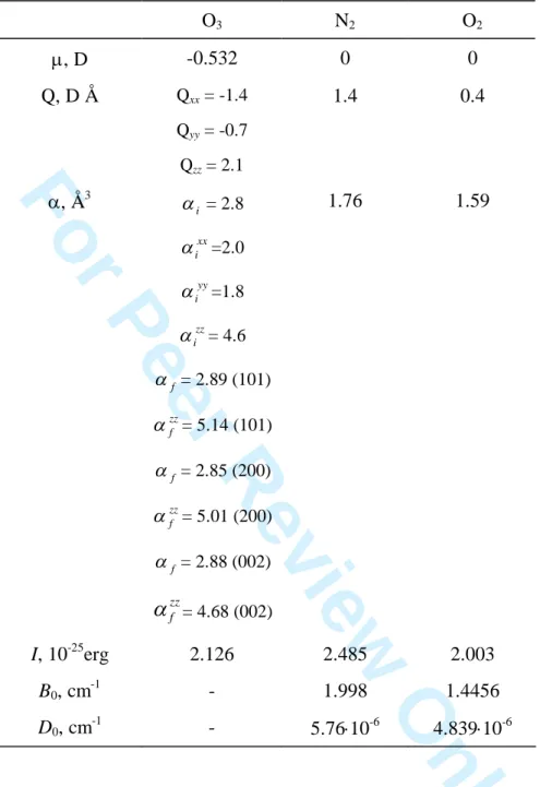
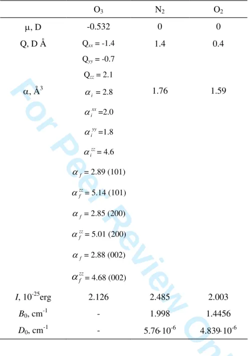
calculate the line shifts due to oxygen pressure. Table 1 gathers molecular and spectroscopic constants for ozone, nitrogen and oxygen used in our calculations.

III. Results and discussion

For the ν1+ν3 band (J = 2–43) calculated O3-N2(O2) line shift coefficients are presented

in Table 2 (lines used for fitting are marked with asterisk) together with the corresponding experimental values from Ref. [5]. These measurements were obtained with the spectral resolution of 0.002 cm-1 and the accuracy of the line shift coefficients estimated at 2.5·10-4cm-1atm-1 (12%) for most lines (15 ≤ J ≤ 30, Ka ≤ 6) and at 4·10-4cm-1atm-1 for

other lines (J < 15, J > 30, Ka > 6). It is clearly seen from this table that the line shifts by

collisions with oxygen molecules are greater than those by collisions with nitrogen molecules. This fact is due to an increasing contribution from S1(b) (which is always

negative) with decreasing interrupting radius b0. By the way, it leads to the corresponding

decrease of the broadening coefficients. Comparison of calculated values with experimental data shows a very good agreement between them: the difference  =  expt -  calc. does not exceed 0.001 cm-1 atm-1 for 98% of O3-N2 lines and 87% of O3-O2 lines with the standard

deviation of 7.04·10-5 cm-1atm-1. The details of statistics are given in Table 3.

The Ka-dependence of the ν1+ν3 band transitions can be seen on Fig. 1 where a

specific combination of the quantum numbers (J + 0.1Ka) allows separation of the lines with identical J-values but different Ka-values (the J-interval starts with J=21 for which Ka=7 and Ka=8 are available). As can be seen from this figure, for some high J

1 2 3 4 5 6 7 8 9 10 11 12 13 14 15 16 17 18 19 20 21 22 23 24 25 26 27 28 29 30 31 32 33 34 35 36 37 38 39 40 41 42 43 44 45 46 47 48 49 50 51 52 53 54 55 56 57 58 59 60

For Peer Review Only

values (J = 26, 31, 32) the calculation reproduces correctly the general behaviour of the experimental Ka-dependences (line shift increases and then decreases with Ka increasing). It is not however the case for other values of J because of the semiempirical character of our model: fitting to some arbitrary chosen experimental values allows a global minimisation of deviations from experimental points but not reproducing fine details in Ka-dependences.

To analyze the vibrational dependence of shifting coefficients, in addition to the band ν1+ν3 two other bands 2ν1 and 2ν3 were studied for the case of nitrogen broadening.

Our theoretical and experimental [6] values for these two bands are given in Tables 4-5. The general comparison of the results for three studied bands shows that the (absolute) line shifts for 2ν1 band are smaller than those of ν1+ν3 and 2ν3 bands. Indeed, because of the

strong polarizability of the ozone molecule the shift becomes noticeable already for transitions to low vibrational states and increases even more for higher vibrational frequencies. A strong vibrational effect and a rotational dependence thus should be noted for the ozone line shifting coefficients. It is difficult to analyse the Ka-dependence for these bands since only in the 2ν1 band and only for two J-values (J = 26, 29) a couple of various Ka values (Ka =0, 1 and Ka =5, 6, respectively) are available. As shows Fig. 2, for these J-values the experimental shifts decrease whereas the calculated shifts increase when passing from Ka =0 (or Ka =5) to Ka =1 (or Ka =6), which can be explained again by the semiempirical character of our approach.

An additional point of our work consisted in evaluation of the temperature dependence of line shifts. The temperature exponents N were determined using the relation

 





N if if T T         297 297   , (8) where if



297



is the shift value at the reference temperature 297 K. This kind of relation is

widely used in the literature and in HITRAN database to characterise the temperature

1 2 3 4 5 6 7 8 9 10 11 12 13 14 15 16 17 18 19 20 21 22 23 24 25 26 27 28 29 30 31 32 33 34 35 36 37 38 39 40 41 42 43 44 45 46 47 48 49 50 51 52 53 54 55 56 57 58 59 60

For Peer Review Only

dependence of the line widths, but mainly for historical reasons since it is valid for molecules interacting through a potential r -η [29–31] and can lead to negative values of the temperature exponents for certain transitions of H2O perturbed by nitrogen, oxygen or air

[32, 33]; for rotational transitions of O3 perturbed by air this relation was found to be

correct for the temperature range 225-350 K but not for the 150-450 K [10]. For the line shifts this relation works well [18] when the shift behaviour with temperature variation is quite regular (Eq. (8) does not describe a change of sign). It is the case for the shifts considered in the present paper. We note for completeness, that a similar formula for the line shift temperature dependence was proposed by Gamache and Rothman [34] which introduces a temperature-dependent sign but is not zero at intermediate temperatures; for our case their expression is equivalent to Eq. (8).

Line shift calculations were carried out for five temperatures (200, 230, 260, 297 and 330 K), and the corresponding N values were extracted by a least-squares fitting procedure. For all studied lines the standard deviation did not exceed 10-6 cm-1atm-1.

Figure 3 shows an example of temperature dependence for the shift of the line 25 5 20  26 5 21 from the ν1+ν3 band (upper panel) and the corresponding plot in logarithmic coordinates (lower panel). The practically linear dependence of ln{δ(T)/δ(297)} on ln(T/297) confirms the validity of Eq. (8) for the temperature dependence of line shifts. For the ν1+ν3 band of O3-N2 system the temperature exponent values are given in Table 2. As can be seen from this table, N varies slightly

from 0.74 to 1.15 for the lines with J = 9 - 43, with the mean value equal to 0.986. It should be noted that these calculations refer to the lines with ΔKa = 0 and ΔKc = 1 (for other

transitions the temperature exponent values can be in principle quite different).

A very rough theoretical estimation of the temperature exponent values for Eq. (8) can be made with the formula obtained by Pickett [35]:

1 2 3 4 5 6 7 8 9 10 11 12 13 14 15 16 17 18 19 20 21 22 23 24 25 26 27 28 29 30 31 32 33 34 35 36 37 38 39 40 41 42 43 44 45 46 47 48 49 50 51 52 53 54 55 56 57 58 59 60

For Peer Review Only

2 2 3 1     N , (9) which gives N =1.5 for the dipole-quadrupole (η = 4) and N =1.375 for

quadrupole-quadrupole (η = 5) interactions. Our results are therefore quite consistent with these estimations.

IV. Conclusions

The comparison of our calculations with experimental values argues that the semiempirical method is quite acceptable for estimating the shifts of ozone vibrotational absorption lines. For this molecule the polarization components of the interaction potential are shown to contribute to the line shift more effectively than the electrostatic dipole-quadrupole interaction (which is very significant for the line broadening). Whereas for the ozone line broadening by nitrogen and oxygen the vibrational effects are very weak, its line shifts demonstrate a strong vibrational dependence. For accurate calculation of ozone line shift coefficients it is therefore necessary to account for this dependence in some components of the ozone polarizability tensor and its polarizability in the excited vibrational states. These components are determined in the present work for (101), (200) and (002) vibrational states by fitting to experimental data. The temperature dependence of the line shifting coefficients is additionally studied. In general, the mechanisms responsible for the ozone line shifting appear to be much more complex than those responsible for the line broadening, which should be permanently kept in mind when calculating its line shape parameters.

The calculated values are intended for use in spectroscopic databases, for example, the "ATMOS" Information System (http://saga.atmos.iao.ru ).

1 2 3 4 5 6 7 8 9 10 11 12 13 14 15 16 17 18 19 20 21 22 23 24 25 26 27 28 29 30 31 32 33 34 35 36 37 38 39 40 41 42 43 44 45 46 47 48 49 50 51 52 53 54 55 56 57 58 59 60

For Peer Review Only

Acknowledgements

The authors acknowledge the financial support by the French national program LEFE-CHAT and by the program "Optical Spectroscopy and Frequency Standards" of the Russian Academy of Sciences.

1 2 3 4 5 6 7 8 9 10 11 12 13 14 15 16 17 18 19 20 21 22 23 24 25 26 27 28 29 30 31 32 33 34 35 36 37 38 39 40 41 42 43 44 45 46 47 48 49 50 51 52 53 54 55 56 57 58 59 60

For Peer Review Only

References

1. M.A.H. Smith, C.P. Rinsland, V. M. Devi, D.C. Benner, and K.B. Thakur, J. Opt. Soc. Am. B 5, 585-592 (1988).

2. M.A.H. Smith, C.P. Rinsland, V. Malathy Devi, E.S. Prochaska, J. Mol. Spectrosc. 164, 239-259 (1994); Erratum, J. Mol. Spectrosc. 165, 596 (1994).

3. M.A.H. Smith, V. Malathy Devi, D.C. Benner, C.P. Rinsland, J. Mol. Spectrosc. 182 (1997) 239-259.

4. V. Malathy Devi, D.C. Benner, M.A.H. Smith, C.P. Rinsland, J. Mol. Spectrosc. 182, 221-238 (1997).

5. A. Barbe, S. Bouazza, J.J. Plateaux, Appl. Opt. 30, 2431-2436 (1991).

6. A. Barbe, J.J. Plateaux, S. Bouazza, Proceedings of the Tenth All-Union Symposium on High Resolution Molecular Spectroscopy, SPIE 1811, Washington, USA, 83-102 (1991).

7. N. Sokabe, M. Hammerich, T. Pedersen, A. Olafsson, J. Henningsen, J. Mol. Spectrosc. 152, 420-433 (1992).

8. R.R. Gamache, L.S. Rothman, Appl. Opt. 24, 1651-1656 (1985). 9. R.R. Gamache, R.W. Davies, J. Mol. Spectrosc. 109, 283-299 (1985).

10. B. J. Drouin, J. Fischer, R.R. Gamache, J. Quant. Spectrosc. Radiat. Transfer 83, 63-81 (2004).

11. A. Bykov, N. Lavrentieva, L. Sinitsa, Mol. Phys. 102, 1653-1658 (2004). 12. J. Buldyreva, N. Lavrentieva, Mol. Phys. 2009 (in press).

13. A. Valentin, Ch. Claveau, A. Bykov, N. Lavrentieva, V. Saveliev, L. Sinitsa, J. Mol. Spectrosc. 198, 218-229 (1999).

14. V. Zeninari, B. Parvitte, D. Courtois, N.N. Lavrentieva, Yu. N. Ponomarev, G. Durry, Mol. Phys. 102, 1697-1706 (2004).

15. A.D. Bykov, N.N. Lavrentieva, T.P. Mishina, L.N. Sinitsa, R.J. Barber, R.N.

1 2 3 4 5 6 7 8 9 10 11 12 13 14 15 16 17 18 19 20 21 22 23 24 25 26 27 28 29 30 31 32 33 34 35 36 37 38 39 40 41 42 43 44 45 46 47 48 49 50 51 52 53 54 55 56 57 58 59 60

For Peer Review Only

Tolchenov, J. Tennyson, J. Quant. Spectrosc. Radiat. Transfer 109, 1834-1844 (2008).

16. J.T. Hodges, D. Lisak, N. Lavrentieva, A. Bykov, L. Sinitsa, J. Tennyson, R.J. Barber, R.N. Tolchenov, J. Mol. Spectrosc. 249, 86-94 (2008).

17. A.D. Bykov, N.N. Lavrentieva, Т.М. Petrova, L.N. Sinitsa, A.M. Solodov, R.J. Barber, J. Tennyson, R.N. Tolchenov, Optika i spectroscop. 105, 25-31 (2008). 18. N. Lavrentieva, A. Osipova, L. Sinitsa, Ch. Claveau, A. Valentin, Mol. Phys. 106,

1261-1266 (2008).

19. N.N. Lavrentieva, T.P. Mishina, L.N. Sinitsa, J. Tennyson, Atm. Oceanic Opt. 21, 1096-1100 (2008).

20. S.A. Tashkun, V.I. Perevalov, J.-L. Teffo, A.D. Bykov, N.N. Lavrentieva, CDSD-1000, J. Quant. Spectrosc. Radiat. Transfer 82, 165-196 (2003).

21. ftp://ftp.iao.ru/pub/CDSD-1000. 22. http://saga.atmos.iao.ru.

23. C.J. Tsao, B. Curnutte, J. Quant. Spectrosc. Radiat. Transfer 2, 41-91 (1962). 24. R.P. Leavitte, J. Chem. Phys. 73, 5432-5450 (1980).

25. A. Bykov, N. Lavrent’eva, and L. Sinitsa, Opt. Spektrosk. 83, 73-82 (1997). 26. A.D. Bykov, N.N. Lavrentieva, Atm. Opt. 4, 518-529 (1991).

27. K.M. Mack, J.S. Muenter, J. Chem. Phys. 66, 5278-5283 (1977).

28. A.Yu. Stepukhin, V.A. Udovenya, L.S. Kostyuchenko, Izv. Vyssh. Uch. Zaved. SSSR, Fizika, Dep. VINITI, No. 2182-B91 (1991).

29. C.H. Townes and A.L. Schawlow, Microwave spectroscopy, McGraw-Hill, New York, NY, 1955.

30. L.D. Landau and E.M. Lifshitz, Quantum Mechanics, Pergamon Press, New York, 1965.

31. P. Varanasi, J. Quant. Spectrosc. Radiat. Transfer 39, 13-25 (1988).

1 2 3 4 5 6 7 8 9 10 11 12 13 14 15 16 17 18 19 20 21 22 23 24 25 26 27 28 29 30 31 32 33 34 35 36 37 38 39 40 41 42 43 44 45 46 47 48 49 50 51 52 53 54 55 56 57 58 59 60

For Peer Review Only

32. G. Wagner, M. Birk, R.R. Gamache, and J.M. Hartmann, J. Quant. Spectrosc. Radiat. Transfer 92, 211-230 (2005).

33. R.A. Toth, L.R. Brown, MA.H. Smith, V. M. Devi, D. C. Benner, M. Dulick, J. Quant. Spectrosc. Radiat. Transfer 101, 339-366 (2006).

34. R.R. Gamache and L.S. Rothman, Abstracts of the Xth Colloquium on High Resolution Molecular Spectroscopy, Dijon, 14-18 September 1987, p. 288.

35. H.M. Pickett, J. Chem. Phys. 73, 6090 (1980).

1 2 3 4 5 6 7 8 9 10 11 12 13 14 15 16 17 18 19 20 21 22 23 24 25 26 27 28 29 30 31 32 33 34 35 36 37 38 39 40 41 42 43 44 45 46 47 48 49 50 51 52 53 54 55 56 57 58 59 60

For Peer Review Only

Table 1. Molecular and spectroscopic constants used in calculations. O3 N2 O2 , D -0.532 0 0 Q, D Å Qxx = -1.4 Qyy = -0.7 Qzz = 2.1 1.4 0.4 , Å3 _i = 2.8 xx i  =2.0 yy i  =1.8 zz i  = 4.6 f  = 2.89 (101) zz f  = 5.14 (101) f  = 2.85 (200) zz f  = 5.01 (200) f  = 2.88 (002) zz f



= 4.68 (002) 1.76 1.59 I, 10-25erg 2.126 2.485 2.003 B0, cm-1 - 1.998 1.4456 D0, cm -1 - 5.7610-6 4.83910-6 1 2 3 4 5 6 7 8 9 10 11 12 13 14 15 16 17 18 19 20 21 22 23 24 25 26 27 28 29 30 31 32 33 34 35 36 37 38 39 40 41 42 43 44 45 46 47 48 49 50 51 52 53 54 55 56 57 58 59 60

For Peer Review Only

Table 2. Calculated and experimental [5] O3-N2(O2) line shift coefficients δ (10-3 cm-1atm-1)

and temperature exponents N for the ν1+ν3 band. Lines used for fitting are marked with

asterisk.

O3-N2 O3-O2 J' Ka' Kc' J Ka Kc

δ calc. δ expt N calc. δ calc. δ expt

42 2 41 43 2 42 -3.28 -4.2 0.78 -4.54 -5.3 38* 5 34 39 5 35 -3.25 -4.0 0.94 -4.69 -4.8 37 4 33 38 4 34 -2.60 -4.0 1.10 -3.73 -4.4 34 6 29 35 6 30 -3.37 -3.6 1.10 -4.71 -4.9 32 5 28 33 5 29 -2.92 -3.3 1.06 -4.22 -4.3 31 6 25 32 6 26 -3.27 -3.6 1.10 -4.53 -4.3 31 5 26 32 5 27 -2.80 -2.7 1.12 -3.99 -3.7 31 1 30 32 1 31 -2.85 -3.8 0.83 -4.06 -4.5 30 5 26 31 5 27 -2.86 -3.7 1.09 -4.15 -4.3 31 0 31 32 0 32 -3.52 -4.4 0.74 -4.76 -4.7 30 1 30 31 1 31 -3.50 -4.2 0.74 -4.76 -4.5 28 6 23 29 6 24 -3.14 -3.5 1.10 -4.37 -3.9 29 0 29 30 0 30 -3.48 -3.2 0.75 -4.72 -4.7 27 6 21 28 6 22 -3.11 -3.0 1.10 -4.33 -3.8 28 2 27 29 2 28 -2.89 -3.5 0.88 -4.12 -4.2 28 1 28 29 1 29 -3.46 -3.1 0.76 -4.71 -4.2 27 1 26 28 1 27 -2.66 -3.3 0.87 -3.82 -4.0 27* 0 27 28 0 28 -3.43 -3.3 0.75 -4.66 -3.8 25 5 20 26 5 21 -2.88 -3.0 1.15 -4.13 -3.4 25 3 22 26 3 23 -2.17 -2.9 1.08 -3.26 -3.5 24 6 19 25 6 20 -3.01 -3.0 1.10 -4.27 -3.3 25 1 24 26 1 25 -2.58 -3.1 0.90 -3.72 -4.0 24 5 20 25 5 21 -2.80 -3.0 1.13 -4.03 -3.5 24 4 21 25 4 22 -2.62 -3.2 1.05 -3.87 -4.0 23 6 17 24 6 18 -2.98 -2.4 1.11 -4.26 -3.5 22* 8 15 23 8 16 -3.24 -3.2 1.04 -4.68 -3.3 23 5 18 24 5 19 -2.78 -2.8 1.13 -4.01 -3.6 22 7 16 23 7 17 -3.14 -2.8 1.07 -4.52 -3.6 23 4 19 24 4 20 -2.38 -2.9 1.13 -3.53 -3.4 22 5 18 23 5 19 -2.73 -3.2 1.12 -3.95 -3.9 21 7 14 22 7 15 -3.10 -3.1 1.06 -4.49 -3.4 23 0 23 24 0 24 -3.27 -3.1 0.79 -4.56 -4.0 20 8 13 21 8 14 -3.14 -3.0 1.02 -4.45 -3.4 20 7 14 21 7 15 -3.06 -3.1 1.05 -4.41 -3.4 19 7 12 20 7 13 -3.02 -2.4 1.04 -3.37 -3.5 14 3 12 15 3 13 -2.25 -2.1 1.01 -3.45 -2.6 10 4 7 11 4 8 -2.28 -1.8 0.99 -3.39 -2.4 8 4 5 9 4 6 -2.25 -2.2 0.94 -3.36 -2.5 3* 2 1 2 2 0 -2.39 -2.0 0.81 -4.66 -1.2 27 0 27 26 0 26 -3.43 — 0.75 -4.53 -3.0 37 6 31 36 6 30 -3.26 — 1.09 -4.01 -3.3 37 2 35 36 2 34 -2.74 -3.2 1.03 -4.54 -3.9 1 2 3 4 5 6 7 8 9 10 11 12 13 14 15 16 17 18 19 20 21 22 23 24 25 26 27 28 29 30 31 32 33 34 35 36 37 38 39 40 41 42 43 44 45 46 47 48 49 50 51 52 53 54 55 56 57 58 59 60

For Peer Review Only

Table 3. Statistics for  =  expt -  calc.values. Percentage of lines Δ , 10-3 cm-1atm-1 O3-N2 O3-O2 Δ 1 98% 87% 1< Δ 2 2% 11% 2< Δ 3 – – 3 < Δ – 2% 1 2 3 4 5 6 7 8 9 10 11 12 13 14 15 16 17 18 19 20 21 22 23 24 25 26 27 28 29 30 31 32 33 34 35 36 37 38 39 40 41 42 43 44 45 46 47 48 49 50 51 52 53 54 55 56 57 58 59 60

For Peer Review Only

Table 4. Calculated and experimental [6] O3-N2 line shift coefficients for the 2ν1 band (10-3

cm-1atm-1). Lines used for fitting are marked with asterisk.

J' Ka' Kc' J Ka Kc calc. expt 25* 6 20 26 7 19 -2.23 -1.9 28 5 23 29 6 24 -2.37 -1.7 14 7 7 15 8 8 -1.71 -1.8 28 4 24 29 5 25 -2.92 -1.5 24 4 20 25 5 21 -2.57 -1.7 29 3 27 30 4 26 -1.12 -1.2 13* 3 11 14 4 10 -2.11 -2.8 43* 1 43 44 0 44 -2.56 -2.5 42 0 42 43 1 43 -2.56 -3.4 18 2 16 19 3 17 -2.60 -2.4 32 0 32 33 1 33 -2.34 -2.2 37 4 34 38 3 35 -0.89 -1.7 25 1 25 26 0 26 -2.13 -1.2 25 2 24 26 1 25 -1.32 -2.7 17 1 17 18 0 18 -1.85 -2.1 12 0 12 13 1 13 -2.52 -1.7 15 2 14 16 1 15 0.04 -2.3 1 2 3 4 5 6 7 8 9 10 11 12 13 14 15 16 17 18 19 20 21 22 23 24 25 26 27 28 29 30 31 32 33 34 35 36 37 38 39 40 41 42 43 44 45 46 47 48 49 50 51 52 53 54 55 56 57 58 59 60

For Peer Review Only

Table 5. Calculated and experimental [6] O3-N2 line shift coefficients for the 2ν3 band (10 -3

cm-1atm-1). Lines used for fitting are marked with asterisk.

J' Ka' Kc' J Ka Kc calc. expt 8* 8 0 9 9 1 -3.95 -4.8 21* 8 14 21 9 13 -6.31 -7.0 26 6 20 26 7 19 -6.20 -6.2 18 6 12 18 7 11 -5.68 -5.2 1 2 3 4 5 6 7 8 9 10 11 12 13 14 15 16 17 18 19 20 21 22 23 24 25 26 27 28 29 30 31 32 33 34 35 36 37 38 39 40 41 42 43 44 45 46 47 48 49 50 51 52 53 54 55 56 57 58 59 60

For Peer Review Only

Figure captions

Figure 1. Calculated and experimental [5] O3-N2 line shifting coefficients for the ν1+ν3

band. The usual abscissa J is incremented by 0.1Ka in order to separate the transitions with identical J but different Ka values.

Figure 2. Calculated and experimental [6] O3-N2 line shifting coefficients for the 2ν1 band.

The usual abscissa J is incremented by 0.1Ka in order to separate the transitions with identical J but different Ka values.

Figure 3. Calculated temperature dependence of the nitrogen-induced 25 5 20  26 5 21 line shift in the ν1+ν3 band (upper panel) and the corresponding plot in logarithmic coordinates used to deduce the N value (lower panel).

1 2 3 4 5 6 7 8 9 10 11 12 13 14 15 16 17 18 19 20 21 22 23 24 25 26 27 28 29 30 31 32 33 34 35 36 37 38 39 40 41 42 43 44 45 46 47 48 49 50 51 52 53 54 55 56 57 58 59 60

For Peer Review Only

-4.5 -4 -3.5 -3 -2.5 -2 21 22 23 24 25 26 27 28 29 30 31 32 33 34

J +0.1K

_a

S

h

if

t,

1

0

-3

cm

-1

a

tm

-1

.

expt

calc

O

₃

-N

₂

ν

1

+ν

3

P-branch

URL: http://mc.manuscriptcentral.com/tandf/tmph 1 2 3 4 5 6 7 8 9 10 11 12 13 14 15 16 17 18 19 20 21 22 23 24 25 26 27 28 29 30 31 32 33 34 35 36 37 38 39 40 41 42 43 44 45 46 47 48 49 50 51 52 53 54 55 56

For Peer Review Only

-3.5

-3

-2.5

-2

-1.5

-1

10

15

20

25

30

35

40

45

J+ 0.1K

a

S

h

if

t, 1

0

-3

c

m

-1

a

tm

-1

.

expt

calc

O

3

-N

2

2ν

1

P-branch

URL: http://mc.manuscriptcentral.com/tandf/tmph 1 2 3 4 5 6 7 8 9 10 11 12 13 14 15 16 17 18 19 20 21 22 23 24 25 26 27 28 29 30 31 32 33 34 35 36 37 38 39 40 41 42 43 44 45 46 47 48 49 50 51 52 53 54 55 56 57 58

For Peer Review Only

-0.1

0.0

0.1

0.2

0.3

0.4

-0.2

-0.1

0.0

0.1

0.2

0.3

0.4

0.5

180

200

220

240

260

280

300

320

340

-4.8

-4.4

-4.0

-3.6

-3.2

-2.8

-2.4

ln

{



(T

)/



(2

9

7

)}

ln{T/297}

S

h

if

t,

cm

-1

a

tm

-1

Temperature, K

1 2 3 4 5 6 7 8 9 10 11 12 13 14 15 16 17 18 19 20 21 22 23 24 25 26 27 28 29 30 31 32 33 34 35 36 37 38 39 40 41 42 43 44 45 46 47 48 49 50 51 52 53 54 55 56 57 58 59 60

For Peer Review Only

Calculations of ozone line shifting induced by N

2

and O

2

pressure

N. Lavrentieva a_{, A. Osipova} b _{and J. Buldyreva} c*

* _{Corresponding author ; Phone: +33 (0)3 81 66 63 60; FAX: +33 (0)3 81 66 64 75; Electronic}

address : jeanna.buldyreva@univ-fcomte.fr

a_{Institute of Atmospheric Optics, 1 ave Akademicheskii, 634055 Tomsk, Russia} b_{Tomsk State University, 36 ave Lenina, 634050, Tomsk, Russia}

c_{Institut UTINAM, UMR CNRS 6213, Université de Franche-Comté, 16 route de Gray,}

25030 Besançon cedex, France 1 2 3 4 5 6 7 8 9 10 11 12 13 14 15 16 17 18 19 20 21 22 23 24 25 26 27 28 29 30 31 32 33 34 35 36 37 38 39 40 41 42 43 44 45 46 47 48 49 50 51 52 53 54 55 56 57 58 59 60

For Peer Review Only

Abstract

Ozone line shifts by nitrogen and oxygen pressure are computed for the ν1+ν3, 2ν1 and

2ν3 bands of the 5µm spectral region by a semiempirical approach. The calculated values

agree with measurements better than 0.001 cm-1atm-1 for 98% of O3-N2 lines and 87% of

O3-O2 lines. In contrast with the water molecule case, the polarization components of the

interaction potential are shown to contribute to the line shift more efficiently than the electrostatic interactions. As intermediate results, the mean dipole polarizability and the components of the polarizability tensor for the vibrational states (101), (200), and (002) of ozone molecule are determined by least-squares fitting of theoretical shifts to some experimental values. The temperature exponents for the ν1+ν3 band lines are also

estimated.

Keywords: ozone, line shift, semiempirical calculation, polarizability in excited vibrational state, temperature exponent

1 2 3 4 5 6 7 8 9 10 11 12 13 14 15 16 17 18 19 20 21 22 23 24 25 26 27 28 29 30 31 32 33 34 35 36 37 38 39 40 41 42 43 44 45 46 47 48 49 50 51 52 53 54 55 56 57 58 59 60

For Peer Review Only

I. Introduction

Among the minor constituents of the Earth’s atmosphere ozone receives a particular attention of scientists due to its double role of protector and pollutant: whereas the stratospheric ozone layer protects the humans, animals and vegetation from the harmful ultraviolet radiation of the Sun, the excessive concentration of ozone in the troposphere is qualified as pollution because of its toxic effects for respiration. Precise measurements of vertical ozone concentration profiles are therefore of crucial importance for health protection services and scientific community interested in comprehension and global modelling of the terrestrial atmosphere.

The probing of atmospheric species is principally realized by non intrusive spectroscopic techniques in the infrared, microwave and millimeter domains. For ozone, the spectral regions of 5 µm and 10 µm are of particular interest since they correspond simultaneously to its most intense absorption bands and to “atmospheric windows” free of water vapour absorption. Reliable inversion of the recorded spectra requires a precise knowledge of ozone spectral line shape parameters (including its main isotopic species) in a wide temperature range and in different vibrational bands.

While the ozone line broadening has been quite intensively studied both experimentally and theoretically, its line shifting data remain quite sparse. Only some measurements were made by Smith et al. [1-4], Barbe et al. [5-6] and Sokabe et al. [7] and only QFT (Quantum Fourier Transform) and ATC (Anderson-Tsao-Curnutte) calculations were realized by Gamache and co-workers [8-9] for N2, O2 and air-broadening. Recently,

the complex-valued version of the Robert-Bonamy formalism was employed by Drouin et al. [10] to estimate line shifts induced by the same perturbers in the rotational band of O3;

no experimental data were reported however for comparison because of their too small values. From the theoretical point of view the line shifting mechanism has a more

1 2 3 4 5 6 7 8 9 10 11 12 13 14 15 16 17 18 19 20 21 22 23 24 25 26 27 28 29 30 31 32 33 34 35 36 37 38 39 40 41 42 43 44 45 46 47 48 49 50 51 52 53 54 55 56 57 58 59 60

For Peer Review Only

complicated character than the line broadening, and many factors negligible for the width become important for the shift (strong dependencies on vibrational quantum numbers, type of perturbing molecules, isotopic species). Since the pressure shift is more sensitive to the intermolecular interaction details than the line broadening, it represents a very promising tool for molecular collision studies. An exhaustive analysis of available experimental data and calculation of line shifts induced in particular by nitrogen and oxygen are therefore of great importance for better understanding of the shifting mechanism and improvement of our knowledge of the ozone spectroscopic properties.

In this paper we present a first systematic calculation of O3-N2(O2) vibrotational line

shifting coefficients and of their temperature dependence for three vibrational bands of the 5µm region (ν1+ν3, 2ν1, 2ν3) by a semiempirical method developed previously [11] and

successfully applied to the case of O3-N2(O2) line broadening [12]. In the frame of this

approach the impact theory is modified by introducing additional semiempirical parameters determined by fitting to experimental data. They are used further to calculate the line shifts which have been not measured. This method gives the possibility to calculate separately the contributions to the line shape parameters from different types of intermolecular interactions and from different scattering channels, which enables an analysis of vibration-rotational dependence of the shifting coefficients for various kinds of perturbers.

II. Method of calculation

The semiempirical method [11] has been already used for calculation of line shape parameters and their temperature exponents for H2O-N2, H2O-O2, H2O-H2O2, СО2-N2 and

CO2-О2 molecular systems [13-20]. In Refs [13-19] it has been shown that for polar active

molecules the semiempirical approach gives quite accurate parameters values. The results of these calculations are actually included in a freely-available carbon dioxide spectroscopic data bank [21] and in the “ATMOS” Information System [22].

1 2 3 4 5 6 7 8 9 10 11 12 13 14 15 16 17 18 19 20 21 22 23 24 25 26 27 28 29 30 31 32 33 34 35 36 37 38 39 40 41 42 43 44 45 46 47 48 49 50 51 52 53 54 55 56 57 58 59 60

For Peer Review Only

In the framework of this approach the line shift corresponding to the radiative transition from the initial state i to the final state f depends on the transition probabilities

D2(ii'|l) and D2(ff'|l) of the different scattering channels connecting the levels i and f with

their neighbouring levels:

) ( )

(

(

)

( )

... ) , ( , 2 , 2 _{′ + ′ +} + =

∑

∑

′ ′ ′ ′ l f f f l i l i i l if B i f D ii l P

ω

D ff l P

ω

δ

(1)

(the higher order terms are neglected). These transition probabilities represent the squared reduced matrix elements of the relevant molecular operators such as the components of the dipole moment (tensorial order l = 1), the components of the quadrupole tensor (l = 2) or the components of higher multipoles. The expansion coefficientsP_l

( )

ω , called in the

literature “interruption” or “efficiency functions”, depend on the intermolecular potential, the trajectory, the energy levels and the wave functions of the perturbing molecule. They can be seen as interruption functions for a given scattering channel and can be formally written as a product of the interruption function of the ATC theory ATC

( )

ω

l

P and of a

correction factor Cl(ω) deduced from fitting to experimental data:

( )

ω

( )

ω ATC

( )

ω l l

l C P

P = . (2)

In order to account for the rotational dependence of the interruption function the form of this correction factor is chosen as

( )

1 2 1 + = J c c Cl ω , (3)

where the fitting parameters c1 and c2 are responsible respectively for the correction of

errors induced by the cut-off procedure and the vibrational dependence. These parameters values c1 = 2.7 and c2 = 7.0 were taken from our previous work [12] on the ν1+ν3 band line

broadening coefficients (fitting to some experimental values from R- and P-branches with various values of the rotational quantum number J) and used here for three considered vibrational bands without any change. This fact confirms the internal consistency of the

1 2 3 4 5 6 7 8 9 10 11 12 13 14 15 16 17 18 19 20 21 22 23 24 25 26 27 28 29 30 31 32 33 34 35 36 37 38 39 40 41 42 43 44 45 46 47 48 49 50 51 52 53 54 55 56 57 58 59 60

For Peer Review Only

semiempirical approach for simultaneous prediction of both line widths and line shifts. The first term B(i, f) appearing in Eq. (1) accounts for the contribution of the isotropic part of the interaction potential:

p vF v b v p i f dv I I I I B c n f i B p i f i f ( ) ( ) ( , , , ) ) ( 2 ) ( 3 ) ( ) , ( 0 3 0 2 2 2 2 2 1

∑

∫

∞ −       + − + − = α µ µ α α ρ , (4) where n is the number density of the perturbing molecules and ρ is the population of their different (rotational) states p, the constant B1 = -3π/(8ħv), and α (α2), µ, Ι (Ι2) are,

respectively, the mean polarizability, dipole moment, and ionization potential of the active (perturbing) molecule. The integration on the relative molecular velocity v is made with the Maxwell-Boltzmann distribution function F(v) and b0 means the interrupting radius. In the

excited vibrational states the mean dipole polarizability is not well known whereas through Eq. (4) it is responsible for the (very clearly pronounced) vibrational dependence of the line shifting coefficient. In our calculations we therefore considered it as an additional fitting parameter.

Equation (1) for the line shift can be expressed in terms of the conventional ATC interruption functions S1(b) and S2(b) which depend on the impact parameter b and

correspond to the contributions from the isotropic and anisotropic parts of the interaction potential, so that S₁

( )

b =B

( )

i, f , (5)

( )

∑

(

) ( )

∑

(

)

( )

′ ′ ′ ′ ′ + ′ = f l f f l i l i i l D ff l P P l i i D b S , 2 , 2 2

ω

ω

. (6) For O3-N2(O2) case the S2(b) contribution can be written as

( )

( ) ( ) ( ) ( ) 20 ( ) 2 02 2 22 2 22 2 12 2 2 b S b S b S b S b S b S = e + e + p + p + p _{, (7)}

where the numerical superscripts denote the multipolarity of the interactions for the active and perturbing molecules and the superscripts e and p denote respectively the electrostatic

1 2 3 4 5 6 7 8 9 10 11 12 13 14 15 16 17 18 19 20 21 22 23 24 25 26 27 28 29 30 31 32 33 34 35 36 37 38 39 40 41 42 43 44 45 46 47 48 49 50 51 52 53 54 55 56 57 58 59 60

For Peer Review Only

and the polarization parts of the interaction potential. Namely, the terms 12 ( ) 2 b S e and ) ( 22 2 b

S e come from the dipole-quadrupole and quadrupole-quadrupole interactions whereas

the terms 22 ( ) 2 b S p , 02 ( ) 2 b S p and 20 ( ) 2 b

S p are due to the polarization and dispersion contributions. Their detailed expressions can be found in [23, 24]. According to Eq. (4) the interruption function S1(b) related to the isotropic potential is determined by µ2f −µi2

andα_f −α_idifferences. The terms 22 ( ) 2 b S p , S₂02p(b) and S₂20p(b) depend on zz i i α α − , zz f f α α − , yy i xx i α α − , and yy f xx f α α − values, where xx f i( ) α , yy f i( ) α , zz f i( )

α are the Cartesian components of the polarizability tensor of the absorbing molecule in the initial (final) states.

In [25] it has been shown that the vibrational dependence of the line shift coefficients of water vapour is explained by the intermolecular potential: the shift is mainly determined by the polarization term S1(b) and the electrostatic termS122 (b)

e _{. In contrast}

with the water vapour molecule, the ozone molecule has a three times smaller dipole moment (0.53 D) while a two times greater mean polarizability (2.8 Å3_{) in the fundamental}

vibrational state. Therefore for O3-N2(O2) interactions the second-order polarization

contributions 22 ( ) 2 b

S p , S₂02p(b) and S₂20p(b) are expected to be significant, and in

addition to the electrostatic terms we accounted in our calculations for the interactions like dipole-induced dipole. The polarization contributions to S2(b) were calculated using the

resonance functions Ig1 and Ig2 determined earlier in [26].

In the present study we have determined the components of the polarizability tensor of the ozone molecule responsible for induction and dispersive interactions. The components for the ground vibrational state were measured in [27] and calculated in [28], the first derivatives of the polarizability with respect to the normal coordinates were also determined, but not the second derivatives necessary for estimating the polarizability in the

1 2 3 4 5 6 7 8 9 10 11 12 13 14 15 16 17 18 19 20 21 22 23 24 25 26 27 28 29 30 31 32 33 34 35 36 37 38 39 40 41 42 43 44 45 46 47 48 49 50 51 52 53 54 55 56 57 58 59 60

For Peer Review Only

excited states. For our purposes, the polarizability in the upper vibrational state α and the _f

zz f

α component of the polarizability tensor were obtained by least-squares fitting to several experimental line shifts induced by nitrogen pressure, for each band separately. Since the

xx- and yy-components have close values, the difference yyf xx

f α

α − was taken equal to its ground vibrational state value. The adjusted parameters α and _f zz

f

α were further used to calculate the line shifts due to oxygen pressure. Table 1 gathers molecular and spectroscopic constants for ozone, nitrogen and oxygen used in our calculations.

III. Results and discussion

For the ν1+ν3 band (J = 2–43) calculated O3-N2(O2) line shift coefficients are

presented in Table 2 (lines used for fitting are marked with asterisk) together with the corresponding experimental values from Ref. [5]. These measurements were obtained with the spectral resolution of 0.002 cm-1 and the accuracy of the line shift coefficients estimated at 2.5·10-4cm-1atm-1 (12%) for most lines (15 ≤ J ≤ 30, Ka ≤ 6) and at 4·10-4cm -1_atm-1 _{for other lines (J < 15, J > 30, K}

a > 6). It is clearly seen from this table that the line

shifts by collisions with oxygen molecules are greater than those by collisions with nitrogen molecules. This fact is due to an increasing contribution from S1(b) (which is

always negative) with decreasing interrupting radius b0. By the way, it leads to the

corresponding decrease of the broadening coefficients. Comparison of calculated values with experimental data shows a very good agreement between them: the difference ∆ = δ

expt _{- δ} calc._{ does not exceed 0.001 cm}-1 _atm-1 _{for 98% of O}

3-N2 lines and 87% of O3-O2

lines with the standard deviation of 7.04·10-5 cm-1atm-1. The details of statistics are given in Table 3.

The Ka-dependence of the ν1+ν3 band transitions can be seen on Fig. 1 where a

specific combination of the quantum numbers (J + 0.1K ) allows separation of the

1 2 3 4 5 6 7 8 9 10 11 12 13 14 15 16 17 18 19 20 21 22 23 24 25 26 27 28 29 30 31 32 33 34 35 36 37 38 39 40 41 42 43 44 45 46 47 48 49 50 51 52 53 54 55 56 57 58 59 60

For Peer Review Only

lines with identical J-values but different Ka-values (the J-interval starts with J=21

for which Ka=7 and Ka=8 are available). As can be seen from this figure, for some

high J values (J = 26, 31, 32) the calculation reproduces correctly the general behaviour of the experimental Ka-dependences (line shift increases and then decreases

with Ka increasing). It is not however the case for other values of J because of the

semiempirical character of our model: fitting to some arbitrary chosen experimental values allows a global minimisation of deviations from experimental points but not reproducing fine details in Ka-dependences.

To analyze the vibrational dependence of shifting coefficients, in addition to the band ν1+ν3 two other bands 2ν1 and 2ν3 were studied for the case of nitrogen broadening.

Our theoretical and experimental [6] values for these two bands are given in Tables 4-5. The general comparison of the results for three studied bands shows that the (absolute) line shifts for 2ν1 band are smaller than those of ν1+ν3 and 2ν3 bands. Indeed, because of the

strong polarizability of the ozone molecule the shift becomes noticeable already for transitions to low vibrational states and increases even more for higher vibrational frequencies. A strong vibrational effect and a rotational dependence thus should be noted for the ozone line shifting coefficients. It is difficult to analyse the Ka-dependence for

these bands since only in the 2ν1 band and only for two J-values (J = 26, 29) a couple

of various Ka values (Ka =0, 1 and Ka =5, 6, respectively) are available. As shows

Fig. 2, for these J-values the experimental shifts decrease whereas the calculated shifts increase when passing from Ka =0 (or Ka =5) to Ka =1 (or Ka =6), which can be

explained again by the semiempirical character of our approach.

An additional point of our work consisted in evaluation of the temperature dependence of line shifts. The temperature exponents N were determined using the relation

( )

if

( )

N if T T −       = 297 297 δ δ , (8) 1 2 3 4 5 6 7 8 9 10 11 12 13 14 15 16 17 18 19 20 21 22 23 24 25 26 27 28 29 30 31 32 33 34 35 36 37 38 39 40 41 42 43 44 45 46 47 48 49 50 51 52 53 54 55 56 57 58 59 60

For Peer Review Only

where δ_if

( )

297 is the shift value at the reference temperature 297 K. This kind of relation is widely used in the literature and in HITRAN database to characterise the temperature dependence of the line widths, but mainly for historical reasons since it is valid for molecules interacting through a potential r -η _{[29–31] and can lead to negative values of the}

temperature exponents for certain transitions of H2O perturbed by nitrogen, oxygen or air

[32, 33]; for rotational transitions of O3 perturbed by air this relation was found to be

correct for the temperature range 225-350 K but not for the 150-450 K [10]. For the line shifts this relation works well [18] when the shift behaviour with temperature variation is quite regular (Eq. (8) does not describe a change of sign). It is the case for the shifts considered in the present paper. We note for completeness, that a similar formula for the line shift temperature dependence was proposed by Gamache and Rothman [34] which introduces a temperature-dependent sign but is not zero at intermediate temperatures; for our case their expression is equivalent to Eq. (8).

Line shift calculations were carried out for five temperatures (200, 230, 260, 297 and 330 K), and the corresponding N values were extracted by a least-squares fitting procedure. For all studied lines the standard deviation did not exceed 10-6 cm-1atm-1.

Figure 3 shows an example of temperature dependence for the shift of the line 25 5 20

← ← ←

← 26 5 21 from the ν1+ν3 band (upper panel) and the corresponding plot in

logarithmic coordinates (lower panel). The practically linear dependence of ln{δ(T)/δ(297)} on ln(T/297) confirms the validity of Eq. (8) for the temperature dependence of line shifts. For the ν1+ν3 band of O3-N2 system the temperature

exponent values are given in Table 2. As can be seen from this table, N varies slightly

from 0.74 to 1.15 for the lines with J = 9 - 43, with the mean value equal to 0.986. It should be noted that these calculations refer to the lines with ∆Ka = 0 and ∆Kc = 1 (for

other transitions the temperature exponent values can be in principle quite different). A very rough theoretical estimation of the temperature exponent values for Eq. (8)

1 2 3 4 5 6 7 8 9 10 11 12 13 14 15 16 17 18 19 20 21 22 23 24 25 26 27 28 29 30 31 32 33 34 35 36 37 38 39 40 41 42 43 44 45 46 47 48 49 50 51 52 53 54 55 56 57 58 59 60

For Peer Review Only

can be made with the formula obtained by Pickett [35]: 2 2 3 1 − + = η N , (9)

which gives N =1.5 for the dipole-quadrupole (η = 4) and N =1.375 for quadrupole-quadrupole (η = 5) interactions. Our results are therefore quite consistent with these estimations.

IV. Conclusions

The comparison of our calculations with experimental values argues that the semiempirical method is quite acceptable for estimating the shifts of ozone vibrotational absorption lines. For this molecule the polarization components of the interaction potential are shown to contribute to the line shift more effectively than the electrostatic dipole-quadrupole interaction (which is very significant for the line broadening). Whereas for the ozone line broadening by nitrogen and oxygen the vibrational effects are very weak, its line shifts demonstrate a strong vibrational dependence. For accurate calculation of ozone line shift coefficients it is therefore necessary to account for this dependence in some components of the ozone polarizability tensor and its polarizability in the excited vibrational states. These components are determined in the present work for (101), (200) and (002) vibrational states by fitting to experimental data.The temperature dependence of the line shifting coefficients is additionally studied. In general, the mechanisms responsible for the ozone line shifting appear to be much more complex than those responsible for the line broadening, which should be permanently kept in mind when calculating its line shape parameters.

The calculated values are intended for use in spectroscopic databases, for example, the "ATMOS" Information System (http://saga.atmos.iao.ru ).

1 2 3 4 5 6 7 8 9 10 11 12 13 14 15 16 17 18 19 20 21 22 23 24 25 26 27 28 29 30 31 32 33 34 35 36 37 38 39 40 41 42 43 44 45 46 47 48 49 50 51 52 53 54 55 56 57 58 59 60

For Peer Review Only

Acknowledgements

The authors acknowledge the financial support by the French national program LEFE-CHAT and by the program "Optical Spectroscopy and Frequency Standards" of the Russian Academy of Sciences.

1 2 3 4 5 6 7 8 9 10 11 12 13 14 15 16 17 18 19 20 21 22 23 24 25 26 27 28 29 30 31 32 33 34 35 36 37 38 39 40 41 42 43 44 45 46 47 48 49 50 51 52 53 54 55 56 57 58 59 60

For Peer Review Only

References

1. M.A.H. Smith, C.P. Rinsland, V. M. Devi, D.C. Benner, and K.B. Thakur, J. Opt. Soc. Am. B 5, 585-592 (1988).

2. M.A.H. Smith, C.P. Rinsland, V. Malathy Devi, E.S. Prochaska, J. Mol. Spectrosc. 164, 239-259 (1994); Erratum, J. Mol. Spectrosc. 165, 596 (1994).

3. M.A.H. Smith, V. Malathy Devi, D.C. Benner, C.P. Rinsland, J. Mol. Spectrosc. 182 (1997) 239-259.

4. V. Malathy Devi, D.C. Benner, M.A.H. Smith, C.P. Rinsland, J. Mol. Spectrosc. 182, 221-238 (1997).

5. A. Barbe, S. Bouazza, J.J. Plateaux, Appl. Opt. 30, 2431-2436 (1991).

6. _{A. Barbe, J.J. Plateaux, S. Bouazza, Proceedings of the Tenth All-Union} Symposium on High Resolution Molecular Spectroscopy, SPIE 1811, Washington, USA, 83-102 (1991).

7. N. Sokabe, M. Hammerich, T. Pedersen, A. Olafsson, J. Henningsen, J. Mol. Spectrosc. 152, 420-433 (1992).

8. R.R. Gamache, L.S. Rothman, Appl. Opt. 24, 1651-1656 (1985). 9. _{R.R. Gamache, R.W. Davies, J. Mol. Spectrosc. 109, 283-299 (1985).}

10. B. J. Drouin, J. Fischer, R.R. Gamache, J. Quant. Spectrosc. Radiat. Transfer 83, 63-81 (2004).

11. A. Bykov, N. Lavrentieva, L. Sinitsa, Mol. Phys. 102, 1653-1658 (2004). 12. _{J. Buldyreva, N. Lavrentieva, Mol. Phys. 2009 (in press).}

13. A. Valentin, Ch. Claveau, A. Bykov, N. Lavrentieva, V. Saveliev, L. Sinitsa, J. Mol. Spectrosc. 198, 218-229 (1999).

14. V. Zeninari, B. Parvitte, D. Courtois, N.N. Lavrentieva, Yu. N. Ponomarev, G. Durry, Mol. Phys. 102, 1697-1706 (2004).

15. A.D. Bykov, N.N. Lavrentieva, T.P. Mishina, L.N. Sinitsa, R.J. Barber, R.N.

1 2 3 4 5 6 7 8 9 10 11 12 13 14 15 16 17 18 19 20 21 22 23 24 25 26 27 28 29 30 31 32 33 34 35 36 37 38 39 40 41 42 43 44 45 46 47 48 49 50 51 52 53 54 55 56 57 58 59 60

For Peer Review Only

Tolchenov, J. Tennyson, J. Quant. Spectrosc. Radiat. Transfer 109, 1834-1844 (2008).

16. _{J.T. Hodges, D. Lisak, N. Lavrentieva, A. Bykov, L. Sinitsa, J. Tennyson, R.J.} Barber, R.N. Tolchenov, J. Mol. Spectrosc. 249, 86-94 (2008).

17. _{A.D. Bykov, N.N. Lavrentieva, Т.М. Petrova, L.N. Sinitsa, A.M. Solodov, R.J.} Barber, J. Tennyson, R.N. Tolchenov, Optika i spectroscop. 105, 25-31 (2008). 18. _{N. Lavrentieva, A. Osipova, L. Sinitsa, Ch. Claveau, A. Valentin, Mol. Phys. 106,}

1261-1266 (2008).

19. _{N.N. Lavrentieva, T.P. Mishina, L.N. Sinitsa, J. Tennyson, Atm. Oceanic Opt. 21,} 1096-1100 (2008).

20. _{S.A. Tashkun, V.I. Perevalov, J.-L. Teffo, A.D. Bykov, N.N. Lavrentieva,} CDSD-1000, J. Quant. Spectrosc. Radiat. Transfer 82, 165-196 (2003).

21. ftp://ftp.iao.ru/pub/CDSD-1000. 22. http://saga.atmos.iao.ru.

23. C.J. Tsao, B. Curnutte, J. Quant. Spectrosc. Radiat. Transfer 2, 41-91 (1962). 24. R.P. Leavitte, J. Chem. Phys. 73, 5432-5450 (1980).

25. A. Bykov, N. Lavrent’eva, and L. Sinitsa, Opt. Spektrosk. 83, 73-82 (1997). 26. _{A.D. Bykov, N.N. Lavrentieva, Atm. Opt. 4, 518-529 (1991).}

27. K.M. Mack, J.S. Muenter, J. Chem. Phys. 66, 5278-5283 (1977).

28. _{A.Yu. Stepukhin, V.A. Udovenya, L.S. Kostyuchenko, Izv. Vyssh. Uch. Zaved.} SSSR, Fizika, Dep. VINITI, No. 2182-B91 (1991).

29. _{C.H. Townes and A.L. Schawlow, Microwave spectroscopy, McGraw-Hill, New} York, NY, 1955.

30. _{L.D. Landau and E.M. Lifshitz, Quantum Mechanics, Pergamon Press, New York,} 1965.

31. _{P. Varanasi, J. Quant. Spectrosc. Radiat. Transfer 39, 13-25 (1988).}

1 2 3 4 5 6 7 8 9 10 11 12 13 14 15 16 17 18 19 20 21 22 23 24 25 26 27 28 29 30 31 32 33 34 35 36 37 38 39 40 41 42 43 44 45 46 47 48 49 50 51 52 53 54 55 56 57 58 59 60