HAL Id: hal-00183259
https://hal.archives-ouvertes.fr/hal-00183259
Submitted on 4 Apr 2020
HAL is a multi-disciplinary open access
archive for the deposit and dissemination of sci-entific research documents, whether they are pub-lished or not. The documents may come from teaching and research institutions in France or abroad, or from public or private research centers.
L’archive ouverte pluridisciplinaire HAL, est destinée au dépôt et à la diffusion de documents scientifiques de niveau recherche, publiés ou non, émanant des établissements d’enseignement et de recherche français ou étrangers, des laboratoires publics ou privés.
Distributed under a Creative Commons Attribution| 4.0 International License
Roller modelling in the context of undertow prediction
Rodrigo Cienfuegos, Eric Barthélemy, Philippe Bonneton
To cite this version:
Rodrigo Cienfuegos, Eric Barthélemy, Philippe Bonneton. Roller modelling in the context of undertow prediction. 29th International Conference on Coastal Engineering, ICCE 2004, Sep 2004, Lisbon, Portugal. pp.318-330, �10.1142/9789812701916_0024�. �hal-00183259�
ROLLER MODELLING IN THE CONTEXT OF UNDERTOW PREDICTION
R. CIENFUEGOS* AND E. BARTHELEMY
Laboratoire des Ecoulements Geophysiques et Industriels BP 53, 38041 Grenoble Cedex 9, France
E-mail: rodrigo. cienfuegos@hmg. inpg.fr
P. BONNETON
Departement de Geologie et d'Oceanographie - Universite de Bordeaux I Av. des Facultes 33405 Talence, France
E-mail: p. bonneton@epoc. u-bordeaux1.fr
In this paper we investigate the energy-based roller equations previously published by Stive and De Vriend (1994) and Dally and Brown (1995). Although these models differ by a factor of 2 in one of their terms, the same parameter values are commonly used to solve them. Our aim is to elucidate these discrepancies and to explore the physical adequacy of the roller models by using an inverse modelling technique based on undertow measurements. Comparison with Cox (1995) experimental data on regular waves propagating on a planar beach shows that a realistic contribution of potential energy in the roller equation should be included.
1. Introduction
Mid to long term prediction of beach profile evolution requires a good esti mation of mean currents in the nearshore zone. For example, the position of the breaking bar is often related to the location of the maximum value of the return current (undertow). Unfortunately, the use of standard wave theories does not provide a correct undertow estimation neither on its max imum intensity, nor on the location for this peak. Based on visual obser vations and shallow water theory, Svendsen (1984) was able to show that the breaking roller contribution in continuity and momentum conservation
*Permanent address : Departamento de Ingenieria Hidniulica y Ambiental, Pontificia Universidad Cat61ica de Chile, Vicuna Mackenna 4860, casilla 306, correo 221, Santiago de Chile. Email : racienfu@ing.puc.cl
equations is far from being negligeable in the surf zone. Using the exper imental data on breaking waves behind an hydrofoil obtained by Duncan ( 1981), Svendsen ( 1984) could relate the cross-sectional roller area to the local wave height and improve the estimation of undertow intensities in the inner surf zone. Nevertheless, this approach cannot reproduce the transi tion zone that exists between the breaking point and the location where the turbulent bore is fully developped. It is evident from many laboratory or field measurements that such a transition zone is always present and is responsible for the landward shift, relative to the breaking point, of set-up and maximum cross-shore and longshore currents (e.g. Bowen et al., 1968; Church and Thornton, 1993). Roelvink and Stive (1989) hypothesized that a lag between turbulence production by the breaking process and dissi pation must be included in order to reproduce the observed shift. One year later, Nairn et al. (1990) showed the theoretical equivalence between the k-equation model written by Roelvink and Stive (1989) and an energy balance equation for the turbulent bore embracing the simple Svendsen's roller concept. The main advantage of the energy-based roller model com pared to the turbulent closure is that roller's contribution can be included in continuity and momentum equations in a straightforward way. For that reason, in recent years the energy balance equation for the roller has been included in several phase-averaged hydrodynamic models used to describe mean current distributions in the nearshore zone (e.g. Reniers and Battjes, 1997; Dally, 2001).
Eventhough from a practical point of view the roller equation does im prove the overall representation of mean cross-shore and longshore currents, the adequacy of its underlying assumptions has not been really checked by comparing its predictions to experimental observations. Accurate labo ratory measurements of roller properties are very difficult to obtain and calibration of roller model parameters must be done by using indirect mea surements (e.g. Dally and Brown, 1995; Walstra et al., 1996). The main drawback of this approach concerns the fact that it is rather difficult to establish whether the wave theory used to describe the "organized motion" or the roller model itself are adequate or not. Bearing the latter in mind, it is possible to understand why two different roller equations can be found in the litterature : Stive and De Vriend (1994) equation (S-DV94 in the following) and Dally and Brown (1995) one (D-B95 in what follows). Sur prinsingly, the same value for the roller parameter, which is associated to the slope of the breaking wave front, is commonly used to run both.
D-B95 models but also assess the physical relevance of the roller concept. We derive the roller equation from a simple energy balance taking care to point out differences with previously published models. Finally, we obtain optimal model parameters by performing inverse modelling on undertow measurements carried out by Cox (1995).
2. The roller equation : an energetic approach
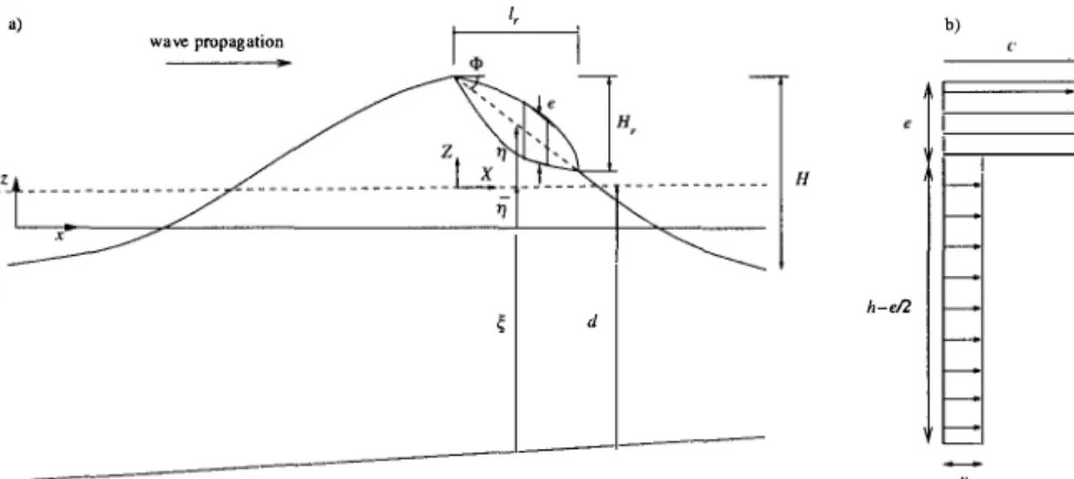
Following Svendsen (1984) we assume a simplified velocity profile as sketched in Fig. 1b, where the breaking roller is simply carried by the waves at the phase velocity c. The layer where the "organized" or mean wave motion takes place has a thickness h- e/2, while the local thickness of the turbulent bore equals e. Here we define a characteristic water depth h = 'TJ + d, where 'T} is the average position of the free surface, and d is the mean water depth. The vertical coordinate of the dividing streamline is z = rj + 'T}-e/2 (where over bar stands for wave-average), while the vertical coordinate of the bottom is z = �- The x-axis coincides with the still wa ter level (positive shorewards), and the z-coordinate is positive upwards. We also introduce local coordinates X, Z for the reference frame moving with the wave (see Fig. 1a). In this moving frame of reference, the average position of the free surface Z = 'TJ can be estimated as
H 'Y
'T] = 2- tan <PX = 2d- tan <PX , for 0 �X � lr, (1) where H is the wave height, <P is the mean breaker angle, 'Y = H / d is the surf zone parameter, and lr is the roller length.
Using now basic principles of fluid mechanics and the assumptions just made, we can write, in the fixed frame of reference, the energy balance equation for the layer where the roller is defined as
{)
1i1+11+ �
{)1i1+11+ �
-8 E dz + -8 [(E + p)c] dz = Dw - Dr,
t
i1+1l-�
X i)+1)-�(2) where E= �PrC2 + Prgz represents the total specific energy, pis the pres sure, Dw and Dr are respectively the total energy dissipation by breaking from "organized" wave motion (source term) and the amount of energy dis sipated from the roller by shearing stresses (sink term). Besides, Pr is the average mass density in the bore region, g is the downward gravitational acceleration and t is the time variable. Consistent with the simplified ve locity profile and the long wave approximation, vertical accelerations are
a) l, wave propagation
1�
b) r- 1-- r-d h-e/2 f----. f----. r-t::::Figure 1. Definition sketch for the breaking roller. a) Variables, b) Assumed velocity distribution.
neglected and an hydrostatic pressure distribution assumed in the roller re gion. Nonetheless, Eq. (2) is not closed and other approximations must be introduced in order to solve it; in particular, we need information about the Dw and Dr terms. In the following, we will use the shallow water approx imation to relate the depth-averaged fluid velocity u to the local position
of the surface elevation in the surf zone and also a slowly varying bottom hypothesis.
2.1. Energy dissipation from the roller
An estimate of the order of magnitude for the amount of energy dissipated from the roller region can be obtained by looking at the work done by shear stresses on the underlying flow (Duncan, 1981). Using the hydrostatic assumption, it can be shown that the local tangential shear stress evaluated at the dividing streamline Z = rJ-e/2 and projected on the line Z = rJ can be written in the moving frame of reference as
1 de
Ts = -prge[2 dX -sin <I> cos <I>] + O(tan3 <I>). (3) This expression is consistent with the one written by Duncan (1981) and by D-B95, but is different from the relation obtained by Deigaard and Freds0e (1989) where O(tan2 <I>) terms are discarded assuming that the breaker angle is small. The total shear required to balance the weight of the roller reads
1lr
dXTs = LT8 = Ts----:i:, = PrgAsin <I>,
0 cos 'J'
where the cross-sectional area of the roller, A, has been introduced and L is the wave length. This expression was first obtained by Duncan (1981).
In the moving frame of reference, the depth-averaged fluid velocity of the underlying "organized" flow is U = u -c. The amount of energy dissipated
from the bore regiona and projected on the x direction should be (of the
order of )
Dr= -UT8 cos�= -(u -c)T8 cos�. (5)
It is important to note here that in previously published roller equations (S-DV94 and D-B95) the flow velocity u was assumed to be negligeable
compared to the wave celerity c; nonetheless, using the long wave approxi mation it can be shown that u can be roughly 20% of the phase speed in the
inner surf zone and even higher near the breaking point. The latter is also sustained by laboratory measurements (e.g Cox, 1995). The wave-averaged energy dissipation from the roller region can then be estimated as
-D _ _ _ d ;r.. � __2 LT8 ;r.. _ _ 2_ prgAsin�cos� r - d C T8 COS '!.' -T COS '*' - 2 T ' +TJ 2+')' +')' (6)
where the definition L = cT (T being the wave period) and the long wave approximation, where u (d + ry) =cry, have been invoked.
2.2. Overall energy dissipated by breaking
Resolution of the Eq. (2) for the roller geometry requires an estimate of the total amount of turbulent kinetic energy available to drive vortical motions. If we follow the energy cascade concept, the term Dw in that equation, which represents the total energy dissipated from the overall flow, can be viewed as the source of energy for large and small scale turbulent motion. In that sense, the rigth hand side of Eq. (2) represents the energy available to drive the roller, which is in fact the largest recognizable vortex in the breaking wave. Even though from a theoretical point of view a turbulent closure should be introduced at this point, the use of the shock theory on the framework of NSWE will allow us to obtain important information about the overall energy dissipated in breaking waves (Bonneton, 2003).
awhich can be viewed as residual turbulent kinetic energy still available to drive smaller scale turbulence.
2.3. Local roller thickness
Wave-averaging some of the left hand side terms of Eq. (2) requires in formation about the local roller thickness e. Here we use Svendsen et al. (2000, SVOO in what follows) exprimental findings by assuming that the local roller thickness can be written in the moving frame of reference as
(X X ) (X 2
e = -K exp - - 1) [(- -1 + - - 1) ],
lr lr lr (7)
where K = (3 exp( -1) -1)-1 A/lr in order to satisfy the additional integral condition A =
J�r
e dX. Thus, it is now necessary to determine the value of the roller length lr.Using the Tollmien mixing layer model, Cointe and Tulin (1994, C-T94 in the following) were able to write a linear relationship between the wave height and the vertical distance between the toe and the top of the roller Hr (see Fig. 1a). In the present context, their expression can be written as
gH _ 1 1 -(32 gHr
?2 - - 2
----;32---;;;-'
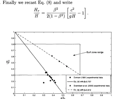
(8)where (3 is an empirical parameter related to the jump in velocity at the toe of the roller. Its value was calibrated using Duncan (1981) experimental data which are representative of small amplitude waves breaking in deep water. We need now to assess its applicability to shallow water conditions. Although there is very little accurate experimental information on roller dynamics in real surf zones, detailed hydrodynamic information on weak hydraulic jumps with Froude numbers similar to those encountered in surf zone waves can be found in SVOO. It seems that the main hypothesis used by C-T94 are reasonably fulfilled in SVOO experimental set-up, i.e. : i) quasi-steady breaker conditions, ii) maximum shear stress occuring on the dividing streamline and being nearly constant over a large extent of the roller, and iii) a shear and velocity discontinuity at its toe. Fig. 2 shows experimental results from Duncan (1981), previously published in C-T94, and experimental data from the three hydraulic jumps studied in SVOO. It can be seen that, at least in the surf zone range, there is also a linear relationship between wave height and roller height in SVOO data but that the empirical parameter (3 is different from the one obtained under deep water conditions. It is remarkable how the SVOO data follow the relationship obtained by C-T94 but more similar experiments should be considered in order to confirm that trend. However, in the present work we will use Eq. (8) and (3 = 0.812 to relate the local wave height to the total roller
height. Finally we recast Eq. (8) and write Hr
(32
[
c2
]
H = 2(1 - /32) gH-
1 . ·,, '· '· '· 0.9 '· '· o.ai--->----.:.>..�---, 0.7 0.6 o/1-0.5 0.4 4. '· '· "' '· '· .... ,,
'· '· '·Surf zone range
0.31---,---'"'-' ---,1
e Duncan (1981) experimental data
0.2 • • • - Eq. (B) with j3=0.707
.. Svendsen et al. (2000) experimental data
0.1
·- ·-· Eq. (8) wllhP,:0.812 0 0 0.1 0.2 0.3 0.4 0.5 0.6 0.7 0.8 0.9
0#-(9)
Figure 2. Wave height v /s total roller height using Duncan (1981) and Svendsen et al. (2000) experimental data.
2.4. Wave-averaged roller equation
Using now hydrostatic and slowly varying bottom assumptions and defini tions for the average position of the free surface (Eq. (1)) and for the local roller thickness (Eq. (7)), we are able to write the wave-averaged roller equation in the monochromatic case. The wave-averaged counterpart of the energy flux term in Eq. (2) can be splitted into kinetic energy, poten tial energy and pressure contributions as follows
Er k
-
-
11J+1J+�
- 2-1 Pre z2
d - r-
-L pc21lr
e dX - r-
-p 2T ' cA1J+1)-�
2 0 (10)17J+7J+�
p g1!"
(
H)
p gAE;= _ e Prgz dz =-t- ('if+77)edX= 'fj+2- aHr �'
7J+7J-2
0c
(11) Er
-11J+1J+�
(- � _ )d _ Pr911" 2
dX _ b A tan <I> Pr9Apr -
-
e Pr9 77 + 77 + 2 z z-2L e - H T '
7J+7J-2
0 r Cwith a = ---,--=-:-:---'-3 -8 exp(-1)
3 exp(-1) -1 and
b = 1 -7 exp(-2)
8[3exp(-1) - 1)]2 The wave-averaged roller equation then reads
where,
[
(
)
-1 Al
1 rj Hr Hr - + - - a- + b - -tan cJ> H 2 H H H H2 ' (13)(3"1 = 2/ ( 2 + ')'), (3q, = sin cJ> cos cJ> and H r / H can be estimated using Eq. ( 9). Careful examination of Eq. (13) shows that S-DV 94 roller model is re covered if Zr = c2 /(2 g), (3"� = 1 and (3q, = tan cJ>. On the other hand, D-B95 roller equation is recovered if Zr = 0 and (3"� = 1. Thus, main differences between both models arise from the treatment of the potential energy /pressure contribution and the small breaker angle approximation made in S-DV 94. Irnplicitely, S-DV 94 assume an equipartition between the kinetic and potential energy /pressure contributions while in D-B95 model the latter is neglected. Despite of that, the same value (3q, = 0.1 is rec ommended to run both models (D-B95; Reniers and Battjes, 1 997). This apparent paradox can be explained by the different wave theories used to describe the "organized" motion. In the next section we will try to im prove integral wave properties estimates by coupling Eq. (13) to a numerical model solving the NSWE and determine optimal breaker angle values. 3. Inverse modelling of � values : application to Cox
(1995) experimental data
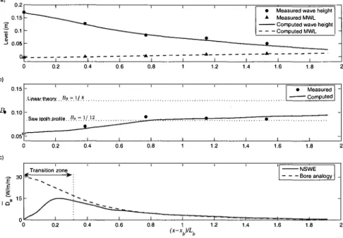
Accurate experimental data on breaking roller dynamics is very difficult to obtain and for practical purposes inverse modelling techniques must be con sidered in order to determine optimal parameter values for roller equations (e.g. D-B95, Walstra et al., 1 996). Since our main objective here is to as sess the physical relevance of Eq. (13), we will use integral wave properties as estimated from a shock-capturing numerical model for the NSWE (Vin cent et al., 2001). A comparison between measured and calculated wave properties in the case of Cox (1 995) experimental data on spilling breaking under regular wave conditions can be seen in Fig. 3. The numerical model gives good estimates for wave height, mean water level and wave shape parameter B0 = ry2 / H2, while overall wave-averaged energy dissipation is
a)
• Measured wave height .& Measured MWL
'E --Computed wave height
I o0�:
- - -Computed MWL0
---·---�---�---�---0.2 0.4 0.6
b)0.15
.Wrle:ar.th�or:y, . J?v.=:'. U .8 ... lb0.10
. Se.w .tooJI:l.prpJUe
..
'!.o. �.�I.��.. .0.8
1.2
1.4
•1.6
1.8
I
• Measured I .. . .. .. --Computed I . .•..0.05
L---�----J_----�---L---L----�----�----�---L---� c)0.2
Transition zone -30
-0.4 0.6
1.15-
�-lo/ ' :
, - -.:::....--0
0
0.2 0.4 0.6
.
0.8
1.2
1.4
0.8
1.2
1.4
1.6
1.8
'I NSWE I I -- - Bore analogy I1.6
1.8
Figure 3. Comparison between measured and computed integral wave properties for Cox (1995) laboratory measurements. Xb is the breaking point coordinate, Lb is the wave length at this location. a) Wave height and mean water level (MWL), b) Wave shape parameter, and c) Wave-averaged energy dissipation in the surf zone.
also well represented converging to the values predicted by the bore anal ogy in the inner surf zone. Additional information on the application of the numerical model to this particular case can be found in Bonneton (2003). In Eq. (13) the only free parameter that remains is the value of the mean breaker angle <I>. Based on recent observations made by Govender et al. (2002) but also on numerical results obtained with Boussinesq models by Schaffer et al. ( 1993) and Kennedy et al. ( 2000), we will consider that <I> is not constant in the surf zone. It should evolve from a maximum value at the breaking point, <l>b, to an equilibrium value, <1>0, in the inner surf zone. Unfortunately, no universal law has been found to relate the breaker angle to local wave properties and we will use the same exponential evolution law as Schaffer et al. (1993),
[
(x- xb)]
where Xb is the horizontal coordinate of the breaking point and lt is a char acteristic length of the transition zone. Therefore, we need to find optimal values for the triplet {<Pb, <1?0, lt}. This can be achieved if we use under tow measurements and mass conservation considerations because continuity equation can be written as
1
!Ztr
1Urc=d z; Ucox(x,z,t)dz=-d(Qw+Qr), (15)
where Urc is the measured undertow, Ucox is the vertical velocity profile
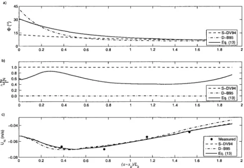
measured by Cox (1995), Zi is the vertical coordinate of the first point of measure and Ztr is the vertical coordinate of the trough level. The right hand side states that the undertow should be equal to the volume flux contributions coming from waves, Qw = B0cH2 /d (using shallow water theory), and from the roller, Qr = A/T. Here we have implicitely assumed that Pr:: Pw, an approximation also used by S-DV94 and D-B95. Because wave-averaged properties have been successfully estimated by the NSWE model (see Fig. 3), and accurate experimental data gives the undertow, the optimal <!?-values can be obtained by inverse modelling using Eq. (15), where Qr is the only remaining unkown quantity. Optimal parameter val ues obtained by minimizing the root mean square error (RMSE)b between computed and measured undertow can be seen in Fig. 4a. Best undertow prediction is reached when { <Pb, <1?0, lt} = {13.0°, 6.5°, Lb/2} using S-DV94 roller equation, and for { <Pb, <1?0, lt} = { 42.0°, 6.0°, Lb/6} in the D-B95 case. On the other hand, Eq. (13) gives an optimal undertow estimate when {<Pb, <P0,lt} = {31.0°, 6.5°, Lb/3}. Associated RMSE are respectively 4.7%, 6.4% and 4.0%.
Eventhough it can be seen in Fig. 4c that very similar results can be obtained with S-DV94 and Eq. (13), the essential point here is to assess which of the models is able to give good undertow predictions by using physically sound parameter values. By looking at Govender et al. (2002) experimental data on mean breaker angle evolution in the surf zone, but also breaking parameter values used by Kennedy et al. (2000) on a fully nonlinear Boussinesq modele, it can be stated that only Eq. (13) behaves in a physically sound way. Moreover, the length of the transition zone given by the parameter value lt = Lb/3 in Eq. (14) coincides roughly with the one estimated from Dw values in Fig. 3c. Thus, it seems that the numerical
bin the domain : 10.0° � <Pb � 45.0° ; 6.0° � <Po � 12.0° ; Lb/15 � lt � Lb/1 .
cunder a constant wave form approximation, it can be shown that <Pb "" 33.0° and
a)
;���-· -
-� --
. .:
__:
1=��!1:
0 0.2 0.4 0.6 0.8 1.2 1.4 1.6 1.8 2
�
!��-::--�_-::::-_-_-::::---�11
0 0.2 0.4 0.6 0.8 1 1.2 1.4 1.6 1.8 2Figure 4. Optimal results as inferred from inverse modelling. a) Evolution of mean breaker angle in the surf zone, b) Ratio of potential energy /pressure and kinetic energy, and c) Comparison between measured and computed undertow.
factor in front of the kinetic energy in roller equation is neither 2, as argued by S-DV94, nor 1 as used in D-B95, but rather an intermediate value as shown in Fig. 4b (where this factor is 1 + 2gZrfc2). This important nu merical finding shows that inside the roller energetic exchanges take place, where a fraction of the potential energy is transformed into kinetic energy while propagating inside the surf zone.
4. Conclusions
Careful examination of an improved version of the roller equation includ ing a realistic flux of potential energy, showed that the main difference between previously published S-DV94 and D-B95 roller models arises from the treatment of potential energy /pressure contribution. While in D-B95 the latter is neglected, S-DV94 implicitely assume an equipartition of ki netic and potential/pressure parts. Using an inverse modelling approach based on accurate estimates of undertow and integral wave properties, we
were able to show that neither the S-DV94, nor the D-B95 energy partition assumptions are realistic. Furthermore, it seems that the "complicated sit uation that occurs when the volume of the roller is changing" evoked in S-DV94 can be explained in a more satisfactory way using energetic argu ments expounded in the present work. Nevertheless, numerical estimation of the potential /pressure contribution is not an easy task and further as sumptions must be introduced. In particular a local reconstruction of the roller geometry is needed which can be obtained using C-T94 theory and SVOO experimental findings. An important result concerning the applica tion of C-T94 theory of steady breakers to weak hydraulic jumps studied in SVOO was also presented. Eventhough this result must be taken with caution because more experimental data on roller dynamics is needed, it could provide useful information to improve breaking parametrizations in time dependent models. Finally, from an engineering point of view, it can be stated that S-DV94 roller equation is more suitable than D-B95 one but that no physical meaning can be attributed to the model parameter (3cp, bearing also in mind that its optimal value will depend on the theory used to describe integral wave properties.
Acknowledgments
This work was partially funded by French research program PATOM. First author would like to thank French Foreign Office, Chilean Research Council (CONICYT) and Pontificia Universidad Cat6lica de Chile for their financial support during his PhD research.
References
P. Bonneton. Nonlinear dynamics of surface waves in the inner surf zone.
Rev. Franr;. Genie Civil, 7(9):1061-1076, 2003.
A.J. Bowen, D.L. Inman, and V.P. Simmons. Wave set-down and set-up. J. Geophys. Res., 73(8):2569-2577, 1968.
J.C. Church and E.B. Thornton. Effects of breaking wave induced turbu lence within a longshore current model. Coastal Eng., 20:1-28, 1993. R. Cointe and M.P. Tulin. A theory of steady breakers. J. Fluid Mech.,
276:1-20, 1994.
D.T. Cox. Experimental and numerical modelling of surf zone hydrodynam ics. PhD. dissertation, University of Delaware, 1995.
W. Dally. Modeling nearshore currents on reef-fronted beaches. Coastal Dynamics'Ol, pages 558-567, 2001.
W . Dally and C.A. Brown. A modelling investigation of the breaking wave roller with application to cross-shore currents. J. Geophys. Res. , 100(C2): 24873-24883, 1995.
R. Deigaard and J. Freds0e. Shear stress distribution in dissipative water waves. Coastal Eng. , 13:357-378, 1989.
J.H. Duncan. An experimental investigation of breaking waves produced by a towed hydrofoil. Proc. R. Soc. London, A, 377:331-348, 1981. K. Govender, G.P. Macke, and M.J. Alport. Video-imaged surf zone wave
and roller structures and flow field. J. Geophys. Res. , 107(C7):9.1-9.21, 2002.
A.B. Kennedy, Q. Chen, J.T. Kirby, and R.A. Dalrymple. Boussinesq modelling of wave transformation, breaking and runup. I: 1D. J. Waterw. Port Coastal and Ocean Eng. , 126(1):39-48, 2000.
R.B. Nairn, J.A. Roelvink, and H.N. Southgate. Transition zone width and implications for modelling surfzone hydrodynamics. 22th. Int. Conf. Coastal Eng . , pages 68-81, 1990.
A.J.H.M. Reniers and J.A. Battjes. A laboratory study of longshore cur rents over barred and non-barred beaches. Coastal Eng., 30:1-22, 1997. J.A. Roelvink and M.J.F. Stive. Bar-generating cross-shore flow mecha
nisms on a beach. J. Geophys. Res., 94(C4):4785-4800, 1989.
H.A. Schaffer, P.A. Madsen, and R.A. Deigaard. A Boussinesq model for waves breaking in shallow water. Coastal Eng., 20:185-202, 1993. O.R. Sorensen and H.A. Schaffer. Wave breaking in a Boussinesq model
with unstructured grids. 28th. Int. Conf. Coastal Eng. , pages 369-379, 2002.
M.J.F. Stive and H.J. De Vriend. Shear stresses and mean flow in shoaling and breaking waves. 24th. Int. Conf. Coastal Eng., pages 594-608, 1994. LA. Svendsen. Mass flux and undertow in a surf zone. Coastal Eng. , 8:
347-365, 1984.
LA. Svendsen, J. Veeramony, J. Bakunin, and J.T. Kirby. The flow in weak turbulent hydraulic jumps. J. Fluid Mech. , 418:25-57, 2000.
S. Vincent, J.-P. Caltagirone, and P. Bonneton. Numerical modelling of bore propagation and run-up on sloping beaches using a MacCormack TVD scheme. J. Hydr. Res., 39(1):41-49, 2001.
D.J.R. Walstra, G.P. Mocke, and F. Smit. Roller contribution as inferred from inverse modelling techniques. 25th. Int. Conf. Coastal Eng., pages