A Direct Search for Dirac Magnetic Monopoles
by
Michael James Mulhearn
Submitted to the Department of Physics
in partial fulfillment of the requirements for the degree of
Doctor of Philosophy
at the
MASSACHUSETTS INSTITUTE OF TECHNOLOGY
Oct 2004
fJIu.e 2Do03(cD
Massachusetts Institute of Technology 2004. All rights reserved.
Author
...
... ...
Department of Physics
October 5, 2004
Certified by... ...Christoph M. E. Paus
Associate Professor
Thesis Supervisor
Accepted
by...
Associate
IMASSACHUS~S INSE OF TECHNOLOGY JUN 2 2 2005 9 ... . ...- ..- -.
- ..
·T- ma
'reytak
Department Head fo ducation
AflcuvtS
A Direct Search for Dirac Magnetic Monopoles
by
Michael James Mulhearn
Submitted to the Department of Physics
on October 5, 2004, in partial fulfillment of the requirements for the degree of
Doctor of Philosophy
Abstract
Magnetic monopoles are highly ionizing and curve in the direction of the magnetic field. A new dedicated magnetic monopole trigger at CDF, which requires large light pulses in the scintillators of the time-of-flight system, remains highly efficient to monopoles while consuming a tiny fraction of the available trigger bandwidth. A specialized offline reconstruction checks the central drift chamber for large dE/dx tracks which do not curve in the plane perpendicular to the magnetic field. We observed zero monopole candidate events in 35.7 pb-1 of proton-antiproton collisions at V/s = 1.96 TeV. This implies a monopole production cross section limit a < 0.2 pb for monopoles with mass between 100 and 700 GeV, and, for a Drell-Yan like pair production mechanism, a mass limit m > 360 GeV.
Thesis Supervisor: Christoph M. E. Paus Title: Associate Professor
Dedication
To those from whom I've wandered for this work: Mom, Dad, Chris, Maricruz, Meg, Doug, and Katie. And to Mila, whom I found along the way.
Acknowledgments
My thesis advisor, Christoph Paus, knew when to leave me alone and when to lift my spinning tires. Gerry Bauer and Sham Sumorok were always willing to listen.
My fellow students shattered the myth of divisive competitiveness at MIT; we worked to get through graduate school together. Ivan Furic was alongside from be-ginning to end. My friends and colleagues at Fermilab gave crucial support and encouragement; the dinner club tempered their's by calling this a "purple elephant search". Daniel Whiteson has consistently given me advice better than his years entitle him to.
The idea for this thesis came from Jonathan Lewis and David Stuart. Jonathan was a key ally from the beginning. Arnd Meyer, Peter Wilson and Bill Badgett were there for the integration. Mathew Jones helped stretch the TOF electronics into a trigger. Eric James wrote new firmware for the muon trigger, Theresa Shaw for the ADMEM, and Carla Pilcher for PreFRED. Philipp Schieferdecker wrote the original GEANT simulation code, and Steve Tether worked out the Runge-Kutta integration. Alex Madorsky designed the TOTRIB and taught me how to write drivers; that was the best part of this thesis.
Contents
1 Introduction
2 Theory
2.1 The Duality Transformation 2.2 Motion in a Magnetic Field 2.3 Dirac's Quantization Condition 2.4 Magnetic-Electric Interactions
2.5 Monopole Pair Production . .
2.6 Ionization and Delta Rays . . 2.7 Multiple Scattering ...
2.8 Cerenkov Radiation ...
3 Tevatron and CDF Detector
3.1 Tevatron ...
3.2 The CDF Detector ...
3.3 Standard Definitions at CDF.
3.4 Central Outer Tracker (COT) 3.5 Time of Flight ...
3.6 The CDF Trigger ...
4 Time-of-Flight Trigger
4.1 TOMAIN and TOF ADMEMs 4.1.1 Technical Description 13 15 15 16 18 20 22 23 25 26 27 28 31 34 36 40 41 45 47 48 . . . .. . .. . . . . .. .. . . .. . . . .. ... . . . . . . . . . . . . . . . . . . . . . . . . . . . . . . . .
4.1.2 Channel Swappers ... 4.1.3 Software ...
4.2 Trigger Cables and Patch Panel ...
4.3 TOTRIB . ...
4.3.1 Technical Description ...
4.3.2 Detector Coverage, Channel Definitions
4.3.3 The Input, Algorithm and Output . . .
4.3.4 VME Interface ...
4.4 Muon Matchbox and Muon PreFRED ...
4.5 BSC-TOF PreFRED ... 4.6 Timing. ... . . . . . . . . . . . . . . . . . . . . . . . . . and Data . . . . . . . . . . . . . . . . . . . . . . . . . .. . . . . Path . . .. . .. . 4.7 Trigger Tables ...
5 Adding Monopoles to GEANT
5.1
Code
Layout
.. ... ... ... .. ... .. ..
5.2 Monopole Tracking ... 5.3 Energy Loss and Delta Rays ... 5.4 Multiple Scattering ...
5.5 Code Validation ...
5.5.1 Comparison with a Stand-Alone Simulation ...
5.5.2 Comparison between analytic and Runge-Kutta solutions 5.6 Summary ...
6 Trigger Efficiency and Dataset
6.1 Acceptance ... 6.2 Electronics Response ... 6.3 Spoilers ... 6.4 Timing. ... 6.5 Digital Response ... 6.6 Dataset ... 50 52 54 56 56 60 63 64 66 67 69 .. 71 73 .. 74 .. 76 .. 78 .. 80 .. 81 .. 81 .. 84 .. 85 93 93 100 105 114 115 118 . . . . . . . . . . . . . . . . . . . . . . . .
...
...
...
...
...
...
7 Candidate Selection 119
7.1 Width Cut . . . 121
7.2 Segment Finding ... 125
8 Results 135
List of Figures
2-1 A monopole-electron collision 19
2-2 The crossing symmetry of monopole-electron interactions ... . 22
2-3 Monopole production cross section ... 23
2-4 Energy loss of monopoles and protons ... ... 25
3-1 3-2 3-3 3-4 3-5 3-6 3-7 4-1 4-2 4-3 4-4 4-5 4-6 4-7 4-8 4-9 4-10 4-11 The Fermilab accelerator complex Peak instantaneous luminosity . . The CDF detector ... CDF tracking sub-detectors . . . COT Wire planes ... COT super-cell . . . .... CDF trigger ... TOF trigger electronics ... TOF ADMEM block schematic . Origin of channel swapping .... The Qietest menu ... TOF trigger cables ... TOF trigger cable shield grounding TOTRIB connector labels .... TOTRIB Block Schematic .... CDF clock signal ... CDF bunch zero signal ... CDF recover signal ... . . . 28 .. . 31 . . . 32 ... 36 ... 37 ... 38 . . . 42 . . . 46 . . . 49 . . . 51 . . . 53 . . . 54 . . . 55 . . . 57 . . . 58 . . . 59 . . . 59 . . . 60
...
...
...
...
...
...
...
CDF halt signal ...
HIP and MIP trigger bit definitions
. . . .60
. . . .61
4-14 TOTRIB coverage ... 61
4-15 TOTRIB data path ... 62
4-16 TOF cosmic trigger algorithm ... 68
4-17 Fine Timing ... 69
4-18 TOF trigger timing diagram ... ... 70
GEANT tracking package ... Monopole tracking algorithm ... Energy loss of protons in air ... Energy loss of monopole in air ... TOF acceptance comparison ... Energy difference at TOF for GEANT and MonSim z difference at TOF for GEANT and MonSim . . . E difference at TOF for GEANT and MonSim . . . Typical r-z trajectory comparison ... Typical E-r trajectory comparison ... Tail r-z trajectory comparison ... Tail E-r trajectory comparison ... Energy difference at TOF for different algorithms . z difference at TOF for different algorithms .... 0 difference at TOF for different algorithms .... TOF acceptance ... TOF acceptance PDF dependence ... TOF acceptance kinematic model dependence . . . Kinematics of m = 200 GeV Monopoles ... Kinematics of m = 400 GeV Monopoles ... Kinematics of m = 700 GeV Monopoles ... TOF data calibration ...
...
74
...
76
...
79
...
80
...
82
...
83
...
84
...
85
...
86
...
87
...
88
...
89
...
90
...
91
...
92
...
94
...
95
...
96
...
97
...
98
...
99
...
101
4-12 4-13 5-1 5-2 5-3 5-4 5-5 5-6 5-7 5-8 5-9 5-10 5-11 5-12 5-13 5-14 5-15 6-1 6-2 6-3 6-4 6-5 6-6 6-7TOF calibrated charge distribution ... Calibrated TOF trigger thresholds ... TOF laser calibration ...
Response function from TOF laser calibration . . Comparison of non-linear behavior ...
Z mass distribution ...
TOF spoilers ...
TOF spoiler luminosity dependence ...
TOF spoiler sum PT dependence ...
TOF pulse arrival times ...
TOF timing window ... TOF timing efficiency ...
The monopole search ...
Corrected COT universal curve ...
COT width response ...
Logarithmic extrapolation of COT width response
COT raw hit distribution ...
Run dependence of COT universal curve ... Segment curvature in Monte Carlo ... Segment q00 in Monte Carlo ...
Segment finding efficiency on high PT tracks . . . Segment finding efficiency with Monte Carlo . . . Background estimate from minimum bias data . . Monopole cross section limit (n = 1) ....
Monopole cross section limit (n = 2) .... Comparison with previous limits ...
Background estimate from trigger data . . .
.103 .104 .106 107 108 .110 . 111 .112 .113 .114 .116 .117 120 122 123 124 126 127 128 129 130 131 133 ... . . 137 ... . . 139 ... . . 140 ... . . 141 8-5 Nearest candidate ... 6-8 6-9 6-10 6-11 6-12 6-13 6-14 6-15 6-16 6-17 6-18 6-19 7-1 7-2 7-3 7-4 7-5 7-6 7-7 7-8 7-9 7-10 7-11 8-1 8-2 8-3 8-4 142 . . . . . . . . . . . . . . . . . . . . . . . . . . . . . . . . . . . . . . . . . . . . . . . . . . . . . . . . . . . . . . . . . . . . . . . . . . . . . . . . . . . . . . . . . . . . . . . . . . . . . . . . . . . . . . . . . . . . . . .
List of Tables
3.1 Accelerator parameters ...
4.1 TOF ADMEM trigger lookup table .
4.2 Simple XTRP algorithm for TOF . .
4.3 BSC-TOF PreFRED bit assignment.
4.4 TOF trigger timing parameters . . . 4.5 Trigger table parameters ...
8.1 Summary of efficiency ... A.1 TOF hardware locations ...
A.2 TOF ADMEM pedestal register addresses . . .
A.3 CDF control signals ...
A.4 Additional CDF control signals ...
A.5 TOTRIB input channel definitions (first 30°) . . A.6 TOTRIB input channel definitions (second 30° )
A.7 TOTRIB input channel definitions (last 30°) . .
A.8 TOTRIB output channel mapping (first 30° ) . .
A.9 TOTRIB output channel mapping (second 30°)
A.10 TOTRIB output channel mapping (last 30° ) . .
A.11 TOTRIB MIP front-panel connector A3 channel mapping. A.12 TOTRIB MIP front-panel connector B3 channel mapping. A.13 TOTRIB CO connector output channel mapping ... A.14 TOTRIB C1 connector output channel mapping ...
...
.143
...
.143
...
.144
...
.144
...
.145
...
.146
...
.146
...
.147
...
.148
...
.149
...
.150
...
.150
...
.151
...
.152
30...
50
...
66
...
67
...
71
...
72
136A.15 TOTRIB VME registers ... 152
A.16 XTRP crack bits . . . 153
Chapter 1
Introduction
The existence of magnetic monopoles would add symmetry to Maxwell's equations [1] without breaking any known physical law. More dramatically, it would make charge
quantization a consequence of angular momentum quantization, as first shown by Dirac [2]. With such appeal, monopoles continue to excite interest and new searches
despite their elusiveness to date.
Grand unified theories predict monopole masses of about 1017 TeV, so there have been extensive searches for high-mass monopoles produced by cosmic rays [3]. Indirect searches for low-mass monopoles have looked for the effects of virtual monopole/anti-monopole loops added to QED Feynman diagrams [4]. Detector materials exposed to radiation from pp collisions at the Tevatron have been examined for trapped monopoles [5]. All results have been negative [6].
This thesis entails a search for Dirac monopoles with mass less than TeV at CDF. By a "Dirac" monopole, we mean a particle without electric charge or hadronic interactions and with magnetic charge g satisfying the Dirac quantization condition:
ge n g = n 68.5 n
hc 2 e 2a
Dirac magnetic monopoles are highly ionizing due to the large value of g. In the CDF detector, they are accelerated in the direction of the solenoidal magnetic field, causing
charged particles, which are circular in the plane perpendicular to the magnetic field. Because of the unique signature from monopoles, it is possible to effectively elim-inate background while maintaining high efficiency. By demonstrating monopole consistent behavior throughout the detector, we expect that a single observed event could be compellingly claimed a discovery.
With such a loud signal, the main challenge of the search is to effectively trigger on magnetic monopoles. CDF cannot possibly record every event, and so physics triggers are needed to make full use of the available luminosity. We have built and commissioned a dedicated highly ionizing particle (HIP) trigger, which requires large light pulses in CDF's Time-of-Flight (TOF) detector. The trigger is highly efficient and consumes a tiny fraction of CDF's bandwidth.
Triggered events are recorded to tape for additional analysis offline. For this search, a specialized reconstruction isolates monopole candidates by checking for ab-normally high ionization and non-curvature in r - using CDF's main tracking chamber.
In the remaining chapters, we discuss the theory of magnetic monopoles, the de-tector and trigger, the monopole simulation, the trigger efficiency, and event selection. We then present results.
Chapter 2
Theory
The original theoretical justification for magnetic monopoles is that they add sym-metry to Maxwell's equations [1] and explain charge quantization in terms of angular momentum quantization. More recently, grand unified theories (GUTs) have pre-dicted the existence of magnetic monopoles, but at masses beyond the reach of any presently conceivable particle accelerator [6, 7].
This chapter explores the new symmetry, the Dirac quantization condition, and a possible production mechanism. The properties of a magnetic monopole, its trajectory and interactions with material, are examined to see how one could be detected.
2.1 The Duality Transformation
The Maxwell equations extended to include magnetic charge take the following form:
(2.1)
V' B =
4Ipm
V
H-
=
ataD+47Fe
As usual, E is the electric field, D the electric displacement, B the magnetic induction, and H the magnetic field. The quantities Pe and je are the familiar electric charge density and electric current density. The addition of magnetic charge introduces Pm and Jm, the magnetic charge density and magnetic current density.
The form of these equations is invariant under a general duality transformation
(e ):
E =E'cos ~ + H' sin
D =D'c os + B'sin~
(2.2)
H =-E'
sin+ H' cos
B
=-D' sin +B' cos
Pe =
plcos
+p sine
sinm
= '"-3
COS
+
i J/sinPm= -P sin + Pm cos m = -je sin ~ + j" cos
The original Maxwell equations are recovered if all particles have the same ratio of magnetic charge to electric charge, which can be set to zero by the right choice of the angle . A useful special case of the duality transformation is when = r/2; the7 extended Maxwell equations are invariant under the replacements
Pe
Pm
3e JmE
H
D
4
B
(2.3)
Pm -Pe 3m -e B -D H -E
This is the transformation meant by "duality" or the "dual" of an EM quantity. Mag-netic charge and electric charge are mirror images of one another, and interchangeable. Apart from being theoretically satisfying, this duality can be used to derive monopole versions of formulas familiar from standard classical electrodynamics.
2.2 Motion in a Magnetic Field
Duality implies a Lorentz force law for a magnetic monopole carrying magnetic charge
g:
A magnetic monopole interacts with a magnetic field as an electron interacts with an electric field.
The general case requires a numerical integration, but the motion in a uniform magnetic field can be solved analytically. Unlike the non-relativistic case, the differ-ential equation
../~?,
up = l
= gB
dt (2.5)
couples the different coordinates due to the presence of 'y in the momentum: Pi =
Ymf i.
We take the uniform magnetic field to be along the z axis, B = Bo02, and start
with the special case of the initial momentum perpendicular to the magnetic field: P = p. An integration of Equation 2.5 leads to
Pz =
ymfz
= gBotPx = tym = O
(2.6) (2.7)
and eliminating gamma gives
f = ? gBot
Po
which can be used to decouple the z and x coordinates to obtain:
D1 ~ gBot
(2.8)
/m2 + p + gBot
0. =Po
v/m2 + p + gBot
One more integration provides the equation of motion:
~~~gBot
et)= Po sinh-1 ° ) z + gB0 Eto (2.9) (2.10) E2o + (gBot)2 -gBowhere Eto = /m 2+ Pxo is the initial transverse energy, equivalent to the total initial
energy in this special case.
momen-turn. Since the monopole is accelerated by the magnetic field, the momentum along the magnetic field will take on every possible value, while the transverse momentum remains constant. This means the general solution can be obtained by translating the special solution in space and time. From the differential equation for the z coordinate, the time translation needed is:
At = po/gBo
(2.11)
Translating the special solution by this amount of time, and moving the origin to t=O we obtain the general solution:
i(t) (sinh- 1(gBo(t +t) - sinh-l( gBoZt (2.12)
gBo Eto Eto
E+ O (gBo(t + At)) 2 (gBo/Žt)2
+
gBO
+EtoEt
-
+This describes a parabola, stretched by relativity, accelerating in the direction of the magnetic field. In the plane perpendicular to the magnetic field, the motion is in a straight line, in sharp contrast to electrically charged particles, which curve in this plane.
2.3 Dirac's Quantization Condition
The classical derivation of Dirac's Quantization Condition [1] is obtained by consid-ering the angular momentum transfered to a magnetic monopole by a collision with
an electron.
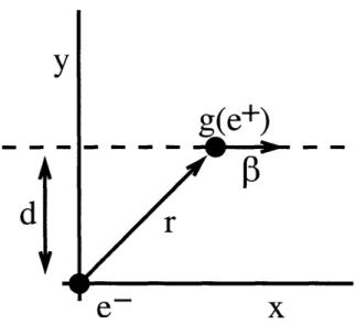
The magnetic monopole moves parallel to the x axis at constant velocity A, inter-acting with the electron located on the origin as shown in Figure 2-1. We consider the case where the impact parameter d is large: a glancing collision.
The force on the magnetic monopole is given by
y
-I
g(e+)
r
e
x
Figure 2-1: A monopole (or positron) makes a glancing collision with an electron
located at the origin.
where the electric field from the electron is
leading to -. I
E = -eT3
-3ged (d2 + (Ct)2) (2.14) (2.15)F = Fy =O
The only non-zero force acting on the monopole is along the z axis, which causes a net impulse
00
F
+00-+
/geddt
Jz=
]t(d2
+ (Ct)2)3
-2eg
cd (2.16)
The angular momentum transfered is
AIL I = -f- x Ap = d ApZ - 2eg (2.17) The Dirac quantization condition is obtained by noting that this angular momentum The Dirac quantization condition is obtained by noting that this angular momentum
A
d
transfer must come in integral quantities of h, leading to: nhc
eg= 2 (2.18)
The Dirac quantization condition implies that
g/e = 2 - 68.5n
(2.19)
This means that the magnetic charge quanta, g, is quite large. For an ion, we write the total electric charge as ze where z is the atomic charge. Likewise, we write the total magnetic charge as ng where n is the quantum number from the Dirac quantization condition.
2.4 Magnetic-Electric Interactions
As a monopole passes through a medium, it interacts with the atoms in the medium. To understand the nature of these magnetic-electric interactions [8], we first consider the effect of the passing monopole in Figure 2-1 on the electron at the origin. To obtain the field of the moving monopole, we find the field of a moving positron, and use duality to obtain the field for a magnetic monopole.
The electromagnetic field at the origin in a frame moving with the positron is given by
Ex e/ t (2.20)
(d
2+
(t)2)ed (2.21)
(d2 + (t)2)2
(2.21)
with all other field components zero. Recalling the Lorentz transformation for electro-magnetic fields in terms of the field parallel (11) and perpendicular () to the velocity
vector [1],
E(1= Ell, E = (1 + x B) (2.22)
B' = Bll, B1 = y(Bi-!3xE) (2.23)
the non-zero field components due to the moving charge at the origin, in the rest frame of the electron, are
e eft (d2 + (t)2)2 (2.24) Eye e-yd (2.25) (d2 ± (3t)2) Be e/d (2.26) (d2 + (t)2)2
We obtain the field for a moving monopole by applying the duality transformation:
Bx = (g/3t (2.27) (d2 + (t)2) ( B9 - -g-yd (2.28) B= (d2+ (t) 2) (.8
E
9=-
g/d
(2.29)
(d2 + (t)2) (2The stationary electron is only affected by the electric fields, and the x averages to zero over the course of the interaction, so the only fields that contribute are Ey for the positron and E9 for the monopole. We obtain the latter with the replacement
e X/ g (2.30)
Under the naive assumption that the isotropy of matter makes the difference in di-rection immaterial, a monopole is effectively a passing particle with electrical charge /3g. There is., however, a correlated response of matter to the passing monopole which becomes increasingly important for slow moving monopoles and dense media [10]. For nearly relativistic monopoles in a gas, the naive treatment is adequate.
2.5 Monopole Pair Production
Duality suggests a new magnetic coupling constant in analogy with the fine structure constant:
g2
ag ]C (2.31)
Due do the large value of g, this coupling constant is larger than one, which makes monopole production non-perturbative. This means that there is no universally ac-cepted prediction from field theory about the production of monopoles.
g
)
)
Y
~~~e
e
Figure 2-2: Monopole pair production is related to monopole-electron scattering by a crossing symmetry.
However, a physically motivated production model has been suggested [5]. We have seen that the interaction of a monopole with an electron merely makes the replacement e -- g. If we imagine how this interaction might look to first order in Quantum Field Theory, we have the diagram on the left of Figure 2-2. But this is related to the Drell-Yan like monopole pair production mechanism, depicted on the right, by a crossing symmetry. It seems reasonable to make the replacement
e - g in the Drell-Yan production mechanism as well. Note that /3, the velocity
of the monopole pairs in the photon rest frame, is a Lorentz invariant, depending only on the mass of the monopoles and the photon mass. Feynman diagram must be manifestly Lorentz invariant!
This Drell-Yan like monopole pair production mechanism is our primary bench-mark. As shown in Figure 2-3, it is the usual Drell-Yan cross section scaled by g/e 2
8
107
106
105
104
03
102
10
10
1
dli102
103
104
10-5
10-6
107
10-8
104
200
400 600
800 1000
Mass [GeV/c
2
]
Figure 2-3: The monopole pair production cross section is obtained from the lepton pair production cross section with the replacement e -+ g. The normal lepton Drell-Yan cross section is scaled by (g/e)2, then convoluted with a 2 factor.
2.6 Ionization and Delta Rays
The energy loss per path-length traveled, dE/dx, due to ionization for a particle with electric charge ze is given by the Bethe-Bloch formula [9],
dE
2KZ
I I
dx ' A 2 2 n
2me/2 y2)
V
2
J
where K = 4rNAr2mec2. The properties of the medium are the atomic number Z, the atomic mass A, and the mean excitation energy I. The constants are the electron
mass me, classical electron radius re and Avogadro's number NA. Typical values are K/A = 0.000307 GeV for A = g mol-1 and I = Z 10 eV. For now, we omit contributions that are significant for small ionization and dense media, referred to as the shell and density corrections.
This formula is derived by considering the impulse imparted to an electron in the material by the passage of the charged particle [1]. As shown in Section 2.4, replacing the EM field tensor for a moving electric charge by its dual shows that the only field component that delivers a net impulse to the electron is an electric field proportional to both the monopole charge ng and its speed . The net effect is to replace ze by ng/3:
dE = (ng/e)2 'Z [ In (2me32 72) 2]. (2.33)
The same conclusion is reached by considering the generalized non-relativistic scatter-ing cross section for small scatterscatter-ing angles [7]. The familiar result for electric-electric scattering (Rutherford scattering),
do, 1 (ze) 2 1
dQ 2m /32 (0/2)4 (2.34) becomes for magnetic-electric scattering
dcr 1__(2__1
dQ-
2m(ng) (/2) (2.35)dQ 2m (0/2) 4 where m is the mass of the light particle.
The ionization energy loss for a magnetic monopole in air is compared to an ordinary charged particle in Figure 2-4. There are two differences: the monopole curve is flatter due to canceling of the 1//2 factor and higher due to the large value of g/e - 68.5. The large ionization energy loss means that the range of monopoles in most solid materials is quite short.
To an electron in matter, a passing monopole is effectively a passing nuclei of charge z n- 68.5 -/. The mean energy loss, energy loss fluctuations, and delta ray production are all different aspects of this interaction. The equations describing these
CL
X
U0a
x
In1
6 1 3Figure 2-4: The energy loss of monopoles and protons in air. phenomena are valid for a wide
range of nuclei, up to z 200. So for small values of n, the replacement ze
-5 ng is justified.
As mentioned above, the correlated response
of matter to a monopole's passage leads to corrections which are important
for small ionization and dense media. A full treatment is provided
by Ref. [lo0].
2.7 Multiple Scattering
The formula for multiple scattering
of monopoles from the nuclei of atoms is deduced in a similar fashion. By exactly
the same exercise as before-replacing
the EM tensor for an electron with its dual-the
monopole multiple scattering
formula differs from 29
the electric equivalent only by the replacement ze -+ ng/. For massive monopoles, the scattering angle is small, and multiple scattering is a small effect.
2.8
erenkov Radiation
Starting with the far fields of a moving charge [1] and applying the duality trans-formation, one obtains the far fields for a moving monopole. The Poynting vector, (E x B)/47r, in the two cases differs only by a substitution of electric with magnetic charge. There is no 3 factor because both the electric and magnetic fields are involved, not just the electric field as in the interactions considered above. For Qerenkov ra-diation, we merely replaces electric charge with magnetic charge (ze - ng). We are again naively ignoring the correlated response of matter, which should lead to a correction, but massive monopoles are not relativistic enough to generate much Cerenkov Radiation, and the naive model is adequate.
Chapter 3
Tevatron and CDF Detector
Fermilab's Tevatron currently produces proton-antiproton (pp) collisions at higher energies than any other experimental facility. It will remain on the energy frontier until experiments at the Large Hadron Collider (LHC) begin taking data in about 2007. The Tevatron collisions occur at two points on an underground ring, which has a radius of about one kilometer. At these collision points are two detectors: the Collider Detector at Fermilab (CDF) and DO. This analysis uses data collected by the CDF experiment.
Between 1997 and 2001, the accelerator complex underwent major upgrades aimed at increasing the luminosity of the accelerator to provide 2 fb- 1of integrated
luminos-ity or more. The upgraded machine accelerates 36 bunches of protons and antiprotons, whereas the original machine accelerated 6 bunches. Consequently, the time between bunch crossings has been decreased from 3.5 pts to 396 ns.
The higher rate operation required major detector upgrades to ensure a fast enough response time. The new electronics is based on a 132 ns clock cycle; this is slightly faster than currently needed, a design choice to accommodate a now un-likely upgrade to an even higher number of bunches.
3.1 Tevatron
Fermilab uses a series of accelerators to produce the high energy pp5 collisions stud-ied at CDF and DO [11]. The paths taken by protons and antiprotons from initial acceleration to collision in the Tevatron are shown in Figure 3-1.
w
D' K AlI
p SOURCE:
-CIIIL= - - 1.
DO
Figure 3-1: The Fermilab accelerator complex.
The Cockcroft-Walton pre-accelerator provides the first stage of acceleration [12]. Inside this device, hydrogen gas is ionized to create H- ions, which are accelerated to 750 keV of kinetic energy. Next, the H- ions enter a linear accelerator (Linac), approximately 500 feet long, where they are accelerated to 400 MeV [13]. An oscillat-ing electric field in the Linac's RF cavities accelerates the ions and groups them into bunches. The ions moving too fast reach the cavity while the electric field is weak, while the ions moving too slow reach the cavity while the electric field is strong.
The 400 MeV H- ions are then injected into the Booster, a circular synchrotron 74.5 m in diameter [13]. A carbon foil strips the electrons from the H- ions at
injection, leaving bare protons. The intensity of the proton beam is increased by injecting new protons into the same orbit as the circulating ones. The protons are accelerated from 400 MeV to 8 GeV by another series of of RF cavities. Each turn around the Booster, the protons gain 500 keV of kinetic energy; but in the steady
state, they lose exactly this much energy through radiation.
To produce antiprotons, protons from the Booster are accelerated to 120 GeV by the Main Injector and directed at a nickel target [11]. In the collisions, about 20 antiprotons are produced per one million protons, with a mean kinetic energy of 8 GeV. The antiprotons are focused by a lithium lens and separated from other particle species by a pulsed magnet. The Main Injector replaced the Main Ring accelerator which was situated in the Tevatron tunnel. The Injector is capable of containing larger proton currents than its predecessor, which results in a higher rate
of antiproton production.
The RF cavities cannot constrain the antiprotons in the plane transverse to the
beam direction. The collider requires narrow beams, so the transverse excursions of the antiprotons must be reduced. Since this process reduces the kinetic energy spread, it is referred to as "cooling" the beam. New batches of antiprotons are initially cooled in the Debuncher synchrotron, collected and further cooled using stochastic cooling [14] in the 8 GeV Accumulator synchrotron. Pickup sensors first sample the average transverse excursions for portions of each bunch. Later, kicker magnets apply correcting forces. This has the effect of damping the antiprotons on average, making a cool narrow beam. It takes between 10 and 20 hours to build up a "stack" of antiprotons which is then used for collisions in the Tevatron. Antiproton availability is most often the limiting factor for attaining high luminosities.
The stochastic cooling is done by the Antiproton Recycler [11], which is also intended to recycle antiprotons when the beam quality has gotten poor after many collisions. The Recycler cools the antiprotons and integrates them with a new stack. Roughly once a day, stacks of protons and antiprotons are transferred to the Main Injector for acceleration to 150 GeV and injection into the Tevatron. The stacks contain 36 bunches, with a proton bunch containing around 3 x 101l protons and an
antiproton bunch containing around 3 x 101° antiprotons. There are more protons because they are more easily produced.
The Tevatron is the last stage of Fermilab's accelerator chain [11]. It receives 150 GeV protons and antiprotons from the Main Injector and accelerates them to 980 GeV. The protons and antiprotons circle the Tevatron in opposite directions. The beams are brought to collision at two "collision points", B0 and DO. The two collider detectors, the Collider Detector at Fermilab (CDF) and DO are built around the collision points.
The luminosity of collisions is given by:
2f(2+r2FNBNpNph
L =f
NB2N
+ F
(at)\i-i
)(3.1)
2?r(o,2± o,) y*
where f is the revolution frequency, NB is the number of bunches, Np/p are the number of protons/antiprotons per bunch, and p/p are the root mean square (RMS) beam sizes at the interaction point. F is a form factor which corrects for the bunch shape and depends on the ratio of (l, the bunch length, to /*, the beta function, at the interaction point. The beta function is a measure of the beam width.
Table 3.1 shows a comparison of Run I accelerator parameters with Run II design parameters [15]. Figure 3-2 shows peak luminosities during the Run II data taking.
Parameter
number of bunches (NB) bunch length [m]
bunch spacing [ns] protons per bunch (Np) antiprotons per bunch (Np)
total antiprotons
i* (cm)
interactions per crossing typical luminosity [cm-2s-1] integrated luminosity [fb-1] record luminosity [cm-2s-1] Run I 6 0.6 3500 2.3 x 10¹¹ 5.5 x 10¹⁰ 3.3 x 10¹¹ 35 2.5 0.16 x 10³ 0.12 Run II 36 0.37 396 2.7 x 10¹¹ 3.0 x 101° 1.1 x 10¹² 35 2.3 0.8 x 1032 4.4 by 2009 1.1 x 1032
Collider Run Ii Peak Luminosity ff -1i 1 i - 1-_t I OQE+32 8 DOE+31 m o c 6 OOE+31 -J IL4 OE+31 200E+31 O,00E+J0 2 WE400 t Zu=11U I ooE+32 B.OOE+31 '. x < 6EOE31 E _1 4 00E+31 0 X 2 00E+31 00OE.O Q e Q $ Q Date
| Peak Luminosity * Peak Lum 20X Average
Figure 3-2: Peak instantaneous luminosity for Run II data taking.
3.2 The CDF Detector
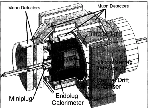
The CDF detector [15] has been upgraded substantially from it's original version [16]. It is designed to detect particles created by pp collisions at the Tevatron's BO interac-tion site and to measure their properties. It is a multipurpose detector, meaning the design is not aimed at one particular physics measurement, but rather at extracting generally useful information about the created particles.
A diagram of the CDF detector is shown in Figure 3-3. A quadrant of the detector is cut out to expose the different sub-detectors. The sub-detector systems are arranged around the beam-pipe, where the pp collisions occur. The beam-pipe is made of beryllium because this metal combines good mechanical qualities with a low nuclear-interaction cross-section.
The first system encountered by a typical particle traversing the CDF detector is the integrated tracking system. The tracking system is barrel-shaped and consists of cylindrical subsystems which are concentric with the beam. It is designed to detect charged particles and measure their momenta and displacements from the point of
Figure 3-3: The CDF detector with a quadrant cut to expose the different sub-detectors.
collision, the primary interaction vertex.
The innermost tracking devices are silicon tracking detectors, which make precise position measurements of the path of a charged particle. A silicon tracking detector is a reverse biased p-n junction. When a charged particle passes through the detector material, it causes ionization. In the semiconductor material, electron-hole pairs are produced. Electrons drift toward the anode, and holes drift toward the cathode, where the charge is gathered. By segmenting the p or n side of the junction into
"strips" and reading out the charge deposition separately on every strip, the position of the charged particle is measured.
A layer of silicon sensors, called Layer 00 (L00), is installed directly onto the beryl-lium beam-pipe, at an average radius of 1.7 cm from the beam [17]. Five concentric layers of silicon sensors (SVX) are located at radii between 2.5 and 10.6 cm [18]. The Intermediate Silicon Layers (ISL) consists of one layer at a radius of 22 cm in the central region and layers at radii 20 and 28 cm in the forward regions [19].
cylindrical open-cell drift chamber with inner and outer radii of 40 and 137 cm. The COT has axial and stereo layers to provide three-dimensional tracking information. The COT is the heart of CDF. Particles are usually first detected in the COT, then
additional information from other detectors is added [20].
The next; system encountered by a typical particle is the Time-of-Flight (TOF) system, designed to provide particle identification for low-momentum charged parti-cles. TOF scintillator bars surround the COT in a barrel shape. The timing infor-mation from the TOF is combined with the momentum measurement from the COT to deduce a particle's mass [21].
Both the tracking and Time of Flight systems are placed inside a superconducting coil, which generates a 1.4 T solenoidal magnetic field. Upon leaving the coil, a typical particle encounters the calorimetry systems, which measure the energy of particles
that shower when interacting with matter.
The CDF sampling calorimeter system [15] uses updated electronics to handle the faster bunch crossings, but the active detector parts were reused without modification. The calorimeter has a projective tower geometry; it is segmented in r and towers that point to the interaction region. The coverage of the calorimetry system is 2r in W and < 4.2 in pseudo-rapidity. The calorimeter system is divided into three regions from smallest r1771 to largest: central, plug and forward. Each calorimeter tower consists of an electromagnetic shower counter followed by a hadron calorimeter. This allows for comparison of the electromagnetic and hadronic energies deposited in each tower, and therefore separation of electrons and photons from hadrons.
The central calorimeters use scintillator as the active detector medium, while the plug and forward calorimeters use gas proportional chambers. The active medium of the electromagnetic calorimeters is alternated with lead sheets, while the hadron calorimeters use layers of iron.
The calorimetry systems are surrounded by muon detector systems. When in-teracting with matter, muons act as minimally ionizing particles; they only deposit small amounts of ionization energy in the material. They are the only particles likely to penetrate both the tracking and calorimeter systems, and leave tracks in the muon
detection system.
The CDF detector has four muon systems [22]: the Central Muon Detector (CMU), Central Muon Upgrade Detector (CMP), Central Muon Extension Detector (CMX), and the Intermediate Muon Detector (IMU). The CMU and CMP detectors are made of drift cells, and the CMX detector is made of drift cells and scintillation counters, which are used to reject background based on timing information. Using the timing information from the drift cells of the muon systems, short tracks (called "stubs") are reconstructed. Tracks reconstructed in the COT are extrapolated to the muon systems. Based on the projected track trajectory in the muon system, the estimated errors on the tracking parameters and the position of the muon stub, a X2 value of the track-stub match is computed. To ensure good quality of muons, an upper limit is placed on the value of X2, the X2 of the track-stub match in the o coordinate.
At the Tevatron, p collisions happen at a rate of 2.5 MHz, and the readout of the full detector produces 250 kB of data. There is no medium available which is capable of recording data this quickly, nor would it be practical to analyze all of this data later on. CDF uses a deadtimeless trigger system to select the most interesting events for the data acquisition system to record.
In this analysis, we use only the Central Outer Tracker, the Time-of-Flight de-tector, and the global data acquisition and trigger system. These are described in greater detail below.
3.3 Standard Definitions at CDF
Because of the barrel-like detector shape, CDF uses a cylindrical coordinate system (r, A, z) with the origin at the center of the detector and the z axis along the nominal direction of the proton beam. The y axis points upward. Since the coordinate system is right-handed, this also defines the direction of the x axis.
Electrically charged particles moving through a solenoidal magnetic field follow helical trajectories. Reconstructed particle trajectories are referred to as "tracks".
The plane perpendicular to the beam is referred to as the "transverse plane", and the transverse momentum of the track is referred to as
PT-As opposed to e+e - collisions, in pp collisions, all of the center of mass energy of the p system is not absorbed in the collision. The colliding partons inside the proton carry only a fraction of the kinetic energy of the proton. As a result, the center of mass system of the parton collisions is boosted along the beam direction (the "longitudinal" direction) by an unknown amount. Quantities defined in the transverse plane are conserved in the collisions. For instance, the sum of all transverse momenta of particles in the collisions is zero (PT = 0).
To uniquely parametrize a helix in three dimensions, five parameters are needed. The CDF coordinate system chooses three of these parameters to describe a
posi-tion, and two more to describe the momentum vector at that position. The three
parameters which describe a position describe the point of closest approach of the helix to the beam line. These parameters are do, p0, and z, which are the p, and z cylindrical coordinates of the point of closest approach of the helix to the beam. The momentum vector is described by the track curvature (C) and the angle of the momentum in the r- z plane (cot 0). From the track curvature we can calculate the transverse momentum. The curvature is signed so that the charge of the particle
matches the charge of the curvature. From cot 0, we can calculate Pz = PT X cot 0.
At any given point of the helix, the track momentum is a tangent to the helix. This means that the angle p0 implicitly defines the direction of the transverse momentum vector at the point of closest approach PT.
The impact parameter (do) of a track is another signed variable; its absolute value corresponds to the distance of closest approach of the track to the beam-line. The sign of do is taken to be that of
P
x d * , where p, d and z are unit vectors in the direction of PT, do and z, respectively.An alternate variable that describes the angle between the z axis and the momen-tum of the particle is pseudo-rapidity () which is defined as:
3.4 Central Outer Tracker (COT)
m 2.0 1.5 1.0 .5 0 TIME OF FLIGHT / 5 LAYERS 30 = 2.0 A= 3.0 30 3o m SILICON LAYERSFigure 3-4: The CDF tracking sub-detectors.
The COT drift chamber provides accurate information in the r - p plane for the measurement of transverse momentum, and substantially less accurate information in the r - z plane for the measurement of the z component of the momentum, z. The COT contains 96 sense wire layers, which are radially grouped into eight "super-layers", as inferred from the end plate section shown in Figure 3-5. Each super-layer is divided in p into "super-cells", and each super-cell has 12 sense wires and a maximum drift distance that is approximately the same for all super-layers. Therefore, the number of super-cells in a given super-layer scales approximately with the radius of the super-layer. The entire COT contains 30,240 sense wires. Approximately half the wires run along the z direction, and are called axial wires. The other half are strung at a small angle (2°) with respect to the z direction, and are called stereo wires. The
small angle stereo wires resolve the z position of a track, making 3D tracking possible. The active volume of the COT begins at a radius of 43 cm from the nominal beam-line and extends out to a radius of 133 cm. The chamber is 310 cm long. Particles originating from the interaction point which have IrI < 1 pass through all 8 super-layers of the COT. Particles which have II < 1.3 pass through 4 or more super-layers. This is a slight simplification; the true acceptance depends on the primary vertex position.
1/th West Endgpate, Gas Side Unis: inches Icm]
R15,980 +-us a l u u ) ful i .C;D m Ou '. L a Mm m C\ ok o Layer # 1 2 3 4 5 6 7 a Gells 18 192 240 288 336 384 432 480
Figure 3-5: The wire planes on a COT end-plate.
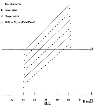
The super-cell layout, shown in Figure 3-6 for super-layer 2, consists of a wire plane containing sense and potential (for field shaping) wires and a field (or cathode) sheet on either side. Both the sense and potential wires are 40 irm diameter gold plated Tungsten. The field sheet is 6.35 ,um thick Mylar with vapor-deposited gold on both sides. Each field sheet is shared with the neighboring super-cell.
The COT is filled with an Argon-Ethane-CF4 (50:35:15) gas mixture. The mixture is chosen to have a constant drift velocity across the cell width. When a charged particle passes through, the gas is ionized. Electrons drift toward the sense wires.
The electric field in a cylindrical system grows exponentially with decreasing radius. As a result, the electric field very close to the sense wire is large, resulting in an avalanche discharge when the charge drifts close to the wire surface. This effect provides a gain of 104 . The maximum electron drift time is approximately 100 ns.
Due to the magnetic field that the COT is immersed in, electrons drift at a Lorentz angle of - 35°. The super-cell is tilted by 35° with respect to the radial direction to compensate for this effect.
| aptalti-x · x I I I I I I 52 54 56 58 60 62 64 R(c SL2
Figure 3-6: The wire layout in a COT super-cell. Here super-layer 2 is depicted.
Signals on the sense wires are processed by the ASDQ (Amplifier, Shaper, Dis-criminator with charge encoding) chip, which provides input protection, amplification, pulse shaping, baseline restoration, discrimination and charge measurement [231. The charge measurement is encoded in the width of the discriminator output pulse, and is used for particle identification by measuring the ionization along the trail of the charge particle (dE/dx). The pulse is sent through 35 ft of micro-coaxial cable, via repeater cards to time-to-digital converter (TDC) boards in the collision hall.
Charged particles leave small charge depositions as they pass through the tracking system. By following, or "tracking" these depositions, pattern recognition algorithms
reconstruct the charged particle track.
There are several pattern recognition algorithms used to reconstruct tracks in the CDF tracking system. Most of the tracks are reconstructed using "Outside-In" algorithms which follow the track from outside of the tracking system inward. This is because the occupancy is much higher toward the center of the detector, making pattern recognition more difficult.
The track is first reconstructed using only COT information. The COT electronics report the hit time and integrated charge for every wire in an event. The hit time is the time that an avalanche occurred at a sense wire. The hit time minus the time of flight is the drift time of the charge in the gas. The time of flight is calculated assuming the particles travel at the speed of light.
The helical track, when projected into the two dimensional r - p plane, is a circle.
This simplifies pattern recognition, so the first step of pattern recognition in the COT looks for circular paths in axial layers of the COT. Super-cells in the axial super-layers are searched for sets of 4 or more hits that fit to a straight line. These sets are called "segments". The straight-line fit for a segment gives sufficient information to extrapolate rough measurements of curvature and 9o0. Once segments are found, they
must be linked together to form tracks. One approach is to link together segments for which the measurements of curvature and T0 are consistent. However, higher occupancy toward the innermost super-layers can cause this approach to fail. Another approach is to improve the curvature and 90 measurement of a segment reconstructed in super-layer 8 by constraining its circular fit to the beam-line, and then adding hits which are consistent with this path. Once a circular path is found in the r - p
plane, segments and hits in the stereo super-layers are added by their proximity to the circular fit. This results in a three-dimensional track fit.
Combined, these two approaches have a high track reconstruction efficiency (a 95%) for tracks which pass through all 8 super-layers (PT > 400 MeV/rmc2 ). The track reconstruction efficiency mostly depends on the local density of tracks. If there are many tracks close to each other, hits from one track can shadow hits from the other track, resulting in efficiency loss.
Once a track is reconstructed in the COT, it is extrapolated into the SVX. Based on the estimated errors on the track parameters, a three-dimensional "road" is formed around the extrapolated track. Starting from the outermost layer, and working in-ward, silicon clusters found inside the road are added to the track. As a cluster gets added, the road gets narrowed according to the knowledge of the updated track pa-rameters. Reducing the width of the road reduces the chance of adding a wrong hit to the track, and also reduces computation time. In the first pass of this algorithm, r - p clusters are added. In the second pass, clusters with stereo information are added to the track.
3.5 Time of Flight
The CDF Time-of-Flight (TOF) system is located just outside the COT, inside the superconducting magnetic coil, as in Figure 3-4. The TOF is designed to distin-guish low-momentum pions, kaons and protons by measuring the time it takes these particles to reach the TOF from the primary vertex. The particle momentum is known from the tracking system, the time-of-flight measurement therefore provides
an indirect measurement of the mass [21].
The TOF is composed of 216 bars of Saint-Gobain (formerly Bicron) BC-408 blue-emitting plastic scintillator, forming an annulus 300 cm long with a radius of 144 cm. The bars have a slightly trapezoidal shape to accommodate the annulus shape, with an approximate width and height of 4 cm.
When fast moving charged particles pass through the scintillator bars, they excite the atoms in the plastic through ionization energy-loss. The excited atoms lose part of this energy by emitting photons of light. Good scintillator materials are characterized by short relaxation times and low attenuation of the generated light.
The scintillator light is converted to a signal voltage by Hamamatsu R5946mod 19-stage fine-mesh photo-multiplier tubes (PMTs) installed on both ends of the scin-tillator bars. The 19-stage high-gain design is needed to ensure adequate gain inside CDF's 1.4 T magnetic field. The photo-multiplier tubes are followed by dual-range
pre-amplifiers before transmission to the readout electronics over shielded twisted pair cables. The dual range increases the dynamic range of the TOF electronics for the magnetic monopole search without adversely effecting the performance for ordi-nary particles. An initial high-gain region for ordiordi-nary tracks is followed by a second low-gain region for larger pulses.
The digitization of the pre-amplified PMT pulses is performed by TOF Transi-tion (TOMAIN) and ADC/Memory (ADMEM) boards. The TOMAIN boards begin ramping an output voltage as soon as the pulse exceeds a threshold, and stop ramping at a common stop signal. The output voltage is digitized by the ADMEMs. Because a large pulse will go above threshold faster than a small pulse, an integrated charge measurement is needed to correct this time-walk effect. The TOMAIN boards inte-grate the charge for a fixed time interval (20 ns for the data in this analysis) after the pulse goes above threshold, then convert the integrated charge to an output current, which is digitized by the ADMEM. The integrated charge measurement is the basis for the TOF highly ionizing particle trigger, used for the monopole search [26].
The timing resolution of the TOF system is about 110 ps for particles crossing the bar exactly in front of one of the photomultiplier tubes. Because light is attenuated in the bar, the timing resolution is worse for tracks crossing far from a PMT.
3.6 The CDF Trigger
Each second, the CDF deadtimeless trigger decides which 50 of 2.5 million events to write to tape. It accomplishes this with a three tiered system, as shown in Figure 3-7, with each level given more time to make a more precise decision. The Level 1 and Level 2 decision are made entirely on fast custom electronics. The Level 3 decision is made with software on off-the-shelf PCs.
After digitizing an event, each sub-detector's front end readout cards store the event data in a digital pipeline. For every 132 ns Tevatron clock cycle, the event is moved up one slot in the pipeline. A small sub-set of the data follows an alternate path to custom electronics, where a Level 1 trigger decision is made. Physics triggers
L1 Storage pipeline: 42 events L2 Buffers 4 events DAQ Buffers Event builder Tevatron: 7.6 MHz crossing rate (132 ns clock cycle) Level 1 latency: 132ns x 42 = 5544 ns < 50 kHz accept rate Level 2: 20ps latency 300 Hz accept rate ejection factor 25000:1
Data storage: nominal freq 30 Hz
Figure 3-7: The CDF trigger.
are combined into a global Level 1 decision, which is sent back to the front end crates just as the event is emerging from the end of the Level 1 pipeline. The decision
arrives 42 events after the event, but because sub-detectors have different intrinsic delays due to cable lengths and other effects, the pipeline length is adjusted to ensure synchronization.
Upon a Level 1 accept, the data for the event is sent to one of four Level 2 buffers, buying additional time for the Level 2 decision. Like the Level 1 pipeline, the
Level 2 buffers are implemented in each sub-detector's front-end readout cards. Some additional information from the front-end cards is included in the Level 2 decision, which must be made quickly enough to clear out buffers for additional Level 1 accepts. Upon a Level 2 accept, the Level 2 buffer is readout from each front end crate, and assembled by the event builder into a complete event. The event is sent to one of 300 Level 3 PCs, where a final software trigger decision is made. At this stage, nearly full event reconstruction is possible.
The Level 1 pipeline has 42 slots, allowing 5 us for the trigger decision. The rejection factor is about 150, so the Level accept rate is below 50 kHz. At Level 2, there are 4 buffers available, allowing 20 ,us for the trigger decision. The Level 2 rejection factor is an addition 150, making the accept rate about 300 Hz. The Level 3 rejection rate is about 10, resulting in 30 events per second written to tape.
Much of the interesting physics at CDF is contained in the trigger. The ability to tag events with displaced vertices, for instance, provides an excellent B-physics sample. The magnetic monopole search uses a custom Level 1 trigger to require high ionization.
Chapter 4
Time-of-Flight Trigger
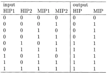
The Time-of-Flight (TOF) trigger provides three Level triggers using the inte-grated charge measurement of photomultiplier tube (PMT) pulses, which is primarily intended to correct discriminator threshold effects on the time measurement. The highly ionizing particle (HIP) trigger checks for abnormally large pulses caused by particles such as magnetic monopoles. The minimum ionizing particle (MIP) mul-tiplicity trigger requires that the total number of normal sized pulses is within a specified range. The TOF cosmic trigger requires two nearly back to back hits in the TOF system [24].
An overview of the TOF trigger hardware is presented in Figure 4-1, and the crate locations are listed in Table A.1. The TOF scintillators form a cylinder around the tracking region; each 15° wedge contains nine TOF scintillator bars. The bars are instrumented on both ends with PMTs and dual-range amplifiers. The pre-amplifiers make the PMT signal more robust for transmission and extend the dynamic range. An initial linear region at high gain is followed by a short non-linear transition region, then a second linear region at lower gain. The high-gain region is intended for typical pulses from ordinary particles, the second low-gain region is to avoid saturation for highly ionizing particles [21, 25, 26, 27].
The digitization of the pre-amplified PMT pulses is done by TOF Transition (TOMAIN) and ADC/Memory (ADMEM) boards. Field Programmable Gate Arrays (FPGAs) in the ADMEMs set trigger bits for pulse heights larger than MIP and HIP
Scintillator Bar
15°F
L
TOMAIN
ADMEM
anch
Pae
-1
IChannel
Swappers
IL
TOTRIB
MTC
BSC Pre-fred
L1 MIP MULTIPLICTY
Muon Matchbox
Muon Pre-fred
~1
L1 HIP TRIGGER
AND COSMIC TRIGGER
Figure 4-1: The TOF trigger electronics for a 15° wedge.
-l
-PMT Oval
Card
A I I ____l t I I -i -"1thresholds.
Additional logic is performed by the special purpose TOF trigger board (TOTRIB), which collects data from TOF ADMEMs and checks for coincidences of pulses above HIP and MIP thresholds on both the east and west sides of TOF scintillator bars. The full coincidence data has five bits per nine TOF scintillator bars, but by com-bining multiple channels, coincidences are calculated at coarser granularity for Level 1 track matching and the TOF cosmic trigger. The TOTRIB also counts the number of MIP coincidences.
HIP east-west coincidences from the TOTRIB are matched to rapidly recon-structed drift chamber tracks using extra channels in the muon trigger system. The high density of inputs to the muon trigger requires the use of serial fiber optic links, prepared by Muon Transition Cards (MTCs). The TOTRIB simplifies the muon match card (Matchbox) programming by providing coincidence data at the same granularity as the extrapolation (four bits per 30°).
At present luminosities, some features of the HIP trigger are not needed to control
the rate. The extrapolation bits are always high, to always satisfy the track matching
requirement. This means that any HIP coincidence causes the trigger to fire. Also,
although the muon match cards report the full coincidence data to the global Level
2 trigger, no special Level 2 trigger is needed. A Level 1 TOF HIP trigger causes an automatic Level 2 and Level 3 accept.
At CDF, each trigger component uses specially programmed Level 1 interface cards, called PreFRED cards, to set the global Level 1 trigger bits appropriately. Because the TOF HIP trigger uses the muon system, the TOF HIP trigger bit is set by the Muon PreFRED. The two TOF MIP triggers use extra channels in the Beam Shower Counter (BSC) PreFRED.
4.1 TOMAIN and TOF ADMEMs
The signal from TOF PMTs is digitized on ADC/Memory (ADMEM) modules. The ADMEM's versatile design is used on various detectors at CDF, mainly calorimetry.