Efficient Sampling through Variable Splitting-inspired Bayesian Hierarchical Models

HAL Id: hal-02438055

https://hal.archives-ouvertes.fr/hal-02438055

Submitted on 14 Jan 2020

HAL is a multi-disciplinary open access

archive for the deposit and dissemination of

sci-entific research documents, whether they are

pub-lished or not. The documents may come from

teaching and research institutions in France or

abroad, or from public or private research centers.

L’archive ouverte pluridisciplinaire HAL, est

destinée au dépôt et à la diffusion de documents

scientifiques de niveau recherche, publiés ou non,

émanant des établissements d’enseignement et de

recherche français ou étrangers, des laboratoires

publics ou privés.

Efficient Sampling through Variable Splitting-inspired

Bayesian Hierarchical Models

Maxime Vono, Nicolas Dobigeon, Pierre Chainais

To cite this version:

Maxime Vono, Nicolas Dobigeon, Pierre Chainais. Efficient Sampling through Variable

Splitting-inspired Bayesian Hierarchical Models. ICASSP 2019 - 2019 IEEE International Conference on

Acous-tics, Speech and Signal Processing (ICASSP), Institute of Electrical and Electronics Engineers (IEEE),

May 2019, Brighton, United Kingdom. pp.5037-5041, �10.1109/ICASSP.2019.8682982�. �hal-02438055�

EFFICIENT SAMPLING THROUGH VARIABLE SPLITTING-INSPIRED

BAYESIAN HIERARCHICAL MODELS

Maxime Vono, Nicolas Dobigeon

University of Toulouse, INP-ENSEEIHT

IRIT, CNRS, Toulouse, France

Pierre Chainais

University of Lille, CNRS, Centrale Lille

UMR 9189 - CRIStAL, Lille, France

ABSTRACT

Markov chain Monte Carlo (MCMC) methods are an important class of computation techniques to solve Bayesian inference problems. Much research has been dedicated to scale these algorithms in high-dimensional settings by relying on powerful optimization tools such as gradient information or proximity operators. In a similar vein, this paper proposes a new Bayesian hierarchical model to solve large scale inference problems by taking inspiration from variable splitting methods. Similarly to the latter, the derived Gibbs sampler permits to divide the initial sampling task into simpler ones. As a result, the proposed Bayesian framework can lead to a faster sampling scheme than state-of-the-art methods by embedding them. The strength of the proposed methodology is illustrated on two often-studied image processing problems.

Index Terms— Bayesian inference, Gibbs sampler, high

dimen-sion, variable splitting.

1. INTRODUCTION

Solving signal/image processing and machine learning problems highly relies on efficient computational methods [1]. Among them, techniques based on variational optimization have received a lot of interest over the past decade leading to fast, efficient and distributed algorithms. For instance, stochastic optimization or Robbins-Monro algorithms [2] and distributed optimization algorithms such as the alternating direction method of multipliers (ADMM), dating back to [3, 4], were successfully resorted to deal with large datasets [5] and high-dimensional problems [6, 7]. As pointed out in [8], Bayesian approaches have not benefited from the same advances as in opti-mization. Nevertheless, by giving the opportunity to explore the posterior distribution of the variable of interest, those methods are of great interest in areas where models must be compared, e.g. for the analysis of gravitational waves [9], or where uncertainties have to be quantified [10]. This complete description of the variable to infer comes at a cost, that can be sometimes prohibitive compared to fast optimization-based techniques. This leads a lot of work to scale Bayesian methods, such as Markov chain Monte Carlo (MCMC) algorithms, enabling them to deal with more and more complex datasets and problems [11]. Among numerous improvements of MCMC methods, optimization-driven approaches attracted the in-terest of a lot of researchers. For instance, gradient information has been successfully used in MCMC methods based on diffusions, e.g. Hamiltonian Monte Carlo methods [12]. In addition, linear pro-gramming has been used to sample efficiently determinantal point processes [13] and convex optimization has been used to explore ef-ficiently possibly non-smooth log-concave probability distributions [14, 15].

In this spirit, this paper proposes a set of methods to solve Bayesian inference problems by taking inspiration from variable splitting techniques. Variable splitting is classically resorted in methods (e.g. the ADMM) to solve large-scale optimization prob-lems by dividing the difficulty over simpler sub-probprob-lems. To this purpose, Section 2 presents how variable splitting can be used within a Bayesian framework and derives an efficient Gibbs sampler where existing state-of-the-art approaches can be embedded. Section 3 shows the results of the proposed approach and of state-of-the-art optimization and MCMC methods applied to image processing prob-lems. Finally, concluding remarks and considered further prospects are reported in Section 4.

2. VARIABLE SPLITTING-INSPIRED BAYESIAN INFERENCE

This section introduces the proposed Bayesian model built from an initial target distribution π and a variable splitting step. The main properties of the derived Bayesian hierarchical model are presented. 2.1. Problem statement

Let consider Bayesian inference problems where we are interested in estimating an unknown object x∈ Rd(e.g. a signal or parameters of a model) from observations y related to the variable to infer through a statistical model with likelihood p(y|x). Within this Bayesian set-ting, the uncertainty on x is modeled via a prior distribution p(x) [16] leading to the posterior distribution

p(x|y) ∝ p(y|x)p(x).

In the sequel, the latter is assumed to have the usual form

π(x)≜ p(x|y) ∝ exp(−f1(x)− f2(x)),

where f1 and f2are two arbitrary functions such that π is well de-fined. Sampling directly from (1) can be difficult for different rea-sons. For instance, if f1and f2are not conjugate, one could rely on more sophisticated sampling schemes, such as Metropolis-Hastings (MH) algorithms [17]. The cost of the latter can be prohibitive in large-scale problems, especially when the likelihood function is a product of terms over a “big” dataset [18]. Additionally, in some cases, some efficient MCMC algorithms cannot be directly applied to sample from π [19]. In these challenging problems, variable split-ting can provide an efficient surrogate method to simplify and/or im-prove the sampling from the target distribution (1). This technique is popular in optimization to tackle the initial difficulty by dividing the cost function f1+ f2in a set of simpler ones. This is achieved by introducing auxiliary variables z to split the objective function. For

θx x y f2 f1 θz z ρ x y f2 ϕρ f1

Fig. 1. DAG associated to the initial Bayesian model (left) and to the proposed model (right). Fixed parameters are represented with dashed circles. θxand θzstand for possible hyperparameters which

are not discussed in this paper.

instance, maximum a posteriori (MAP) estimation under (1) leads to the optimization problem

arg min

x∈Rd

f1(x) + f2(x), (1) which can be rewritten using variable splitting as

arg min

x∈Rd_,z∈Rd

f1(x) + f2(z) s.t. x = z. ₍₂₎

This new formulation of MAP estimation yields several (two in this case) optimization sub-problems, one for each variable where f1and

f2are dissociated [5].

2.2. Bayesian hierarchical model

Following this variable splitting trick, an auxiliary variable z∈ Rd_is

introduced to simplify the sampling from π. Thus sampling from the latter will be replaced by sampling from two simpler distributions (6) and (7). To this aim, let us consider a Bayesian hierarchical model through a joint distribution πρ(x, z) defined by

πρ(x, z)∝ exp

(

−f1(x)− f2(z)− ϕρ(x, z)

)

, (3) where ρ > 0 and ϕρstands for a divergence where the discrepancy

between x and z is controlled by ρ. Of course, ϕρhas to be chosen

such that πρand its related probability distributions are

Lebesgue-integrable. Possible choices for ϕρ, that can be viewed as a coupling

function, are discussed in Section 2.3. In cases where f1and f2stand for potential functions associated to the likelihood and to the prior respectively, fig.1 shows the directed acyclic graph (DAG) related to the proposed split model.

In general, the split distribution πρin (3) does not correspond

to an augmentation of the initial target distribution π. Thereby, the marginal distribution of x under πρstands for an approximation of

π. The corresponding approximation error, controlled by ρ, can be

made arbitrarily small as depicted by Theorem 1 proven in [20]. Theorem 1 [20, Theorem 1] Let pρ =

∫

Rdπρ(x, z)dz be the

marginal of x under πρ. Assume that in the limiting case ρ→ 0, ϕρ

is such that exp(−ϕρ(x, z) ) ∫ Rdexp ( −ϕρ(x, z) ) dx−−−→ρ→0 δx(z) (4)

Then, under (4) and by assuming that f1and f2are lower-bounded,

pρcoincides with π when ρ→ 0, that is

∥pρ− π∥_TV−−−→

ρ→0 0. (5)

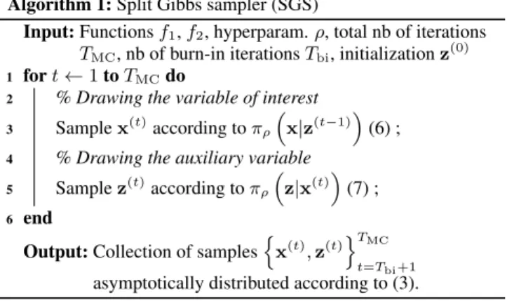
Algorithm 1:Split Gibbs sampler (SGS)

Input:Functions f1, f2, hyperparam. ρ, total nb of iterations

TMC, nb of burn-in iterations Tbi, initialization z(0)

1 for t← 1 to TMCdo

2 % Drawing the variable of interest 3 Sample x(t)according to πρ

(

x|z(t−1)

) (6) ;

4 % Drawing the auxiliary variable 5 Sample z(t)according to πρ

(

z|x(t))_{(7) ;}

6 end

Output:Collection of samples {

x(t), z(t)

}TMC

t=Tbi+1

asymptotically distributed according to (3).

Generalizations of the proposed split scheme and more details can be found in [20, 21].

2.3. Gibbs sampler

The conditional distributions under the split distribution πρwrite

πρ(x|z) ∝ exp ( −f1(x)− ϕρ(x, z) ) (6) πρ(z|x) ∝ exp ( −f2(z)− ϕρ(x, z) ) . (7) Thus, the variable of interest x can be estimated through Gibbs sam-pling where each samsam-pling step does not involve f1 + f2but only a part of this initial potential function f1or f2. Strong similarities with distributed optimization algorithms, e.g. the ADMM, are dis-cussed in [20]. The Gibbs sampler derived to sample from the split distribution πρ is depicted in algo. 1 and called split Gibbs

sam-pler (SGS). Our motivation to introduce variable splitting was the simplification of the inference and the derivation of a more efficient sampling scheme. To this purpose, the conditional distributions (6) and (7) must be simple to sample from compared to the sampling from π. Depending on the form and properties (e.g. convexity, differentiability) of the potential functions f1 and f2, the coupling function can be adaptively chosen. For instance, [20, 22] consider

ϕρ(x) = (2ρ2)−1∥x − z∥2₂for its gradient Lipschitz,

differentia-bility and convexity properties while [21] invokes conjugacy argu-ments to choose ϕρ. For a detailed discussion on the Gibbs sampling

procedure, we refer the reader to [20, Section III.A]. 3. EXPERIMENTS

This section illustrates the application of the proposed Bayesian framework on two linear Gaussian inverse problems encountered in image processing, namely image deblurring using either a total variation (TV) prior or a frame-based approach.

3.1. Linear Gaussian inverse problems

By considering either an analysis or a synthesis approach [23], linear Gaussian inverse problems involve the estimation of an unknown object x through the forward model

y = Px + n, (8)

where P is a direct operator and n ∼ N (

0d, σ2Id

)

stands for noise. If f1denotes the potential associated to the likelihood, then for all x∈ Rd_,

f1(x) = 1

2σ2∥y − Px∥ 2

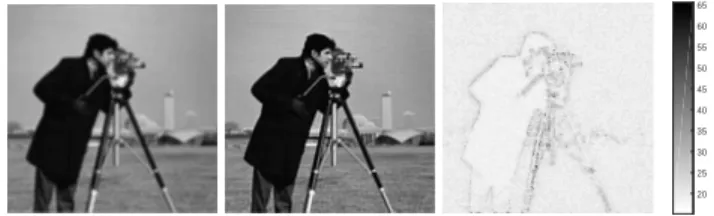
Fig. 2. Image deblurring with TV prior. (left) Original image, (mid-dle) noisy and blurred image and (right) MMSE estimate computed with SGS.

By taking, as in [20], ϕρ(x) =

1

2ρ2∥x − z∥ 2

2and by assuming that for all x∈ Rd, the potential f2associated to the prior writes

f2(x) = τ ψ(x), τ > 0, (10) the conditional distributions (6) and (7) have the form

πρ(x|z) = N ( µx, Qx−1 ) (11) πρ(z|x) ∝ exp ( −τψ(z) − 1 2ρ2∥z − x∥ 2 2 ) , where (12)          Qx= 1 σ2P T P + 1 ρ2Id (13) µ_x= Qx−1 ( 1 σ2P T y + 1 ρ2z ) . (14) If the matrix P can be diagonalizable in a certain domain (e.g. Fourier domain), then sampling from (11) can be performed effi-ciently in this domain through the exact perturbation-optimization (E-PO) algorithm [24]. Additionally, if ψ corresponds to a con-vex and possibly non-smooth regularization function (e.g. TV), sampling from (12) can be conducted using the proximal MCMC algorithm P-MYULA which has well-understood theoretical prop-erties.

3.2. Image deblurring with total variation prior

Problem formulation –In this first experiment, we consider an image deconvolution problem where an original image x of size 256× 256 (d = 65536) is blurred via a 5×5 Gaussian blur kernel with standard deviation equal to 2, see fig. 2. Thereby, the cor-responding operator P = B is a circulant matrix, diagonalizable in the Fourier domain. The regularization potential ψ is the total variation (TV) function.

Experimental design – The proposed method is compared with the state-of-the-art proximal MCMC algorithm, namely proximal Moreau-Yoshida unadjusted Langevin algorithm (P-MYULA) [15]. Additionally, SGS and P-MYULA will be compared with their counterpart optimization algorithms namely the split augmented Lagrangian shrinkage algorithm (SALSA) [6] and the fast iterative shrinkage thresholding algorithm (FISTA) [25], respectively. The variance σ2of the Gaussian noise is set such that the signal-to-noise ratio (SNR) is equal to 40dB. The Lipschitz constant Lf1associated

to ∇f1, needed to launch FISTA and P-MYULA, is defined by

Lf1 = σ

−2_λmax(PT_{P) where λmax(P}T_{P) stands for the largest}

eigenvalue of PTP.

Since SGS and P-MYULA do not target the same stationary dis-tribution, comparing explicitly these two algorithms is not straight-forward and highly depends on the reconstruction criteria used by the practitioner. Nethertheless, this experiment aims to demonstrate

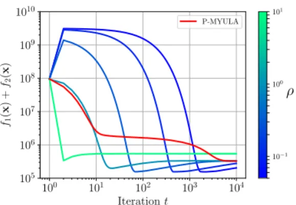
100 ₁₀1 ₁₀2 ₁₀3 ₁₀4 Iteration t 105 106 107 108 109 1010 f1 (x ) + f2 (x ) P-MYULA 10−1 100 101 ρ

Fig. 3. Image deblurring with TV prior. Convergence of the Markov chains associated to SGS w.r.t ρ (fromguppie greentoblue) and P-MYULA (red) toward the typical set of π.

that SGS, by embedding P-MYULA, can lead to reliable approxi-mate estiapproxi-mates with a lower computational cost.

The number of MCMC iterations has been set to TMC= 1.1× 104_{with Tbi= 10}3_{burn-in iterations for SGS. For P-MYULA, due} to slower mixing properties (see fig. 4), the number of MCMC it-erations has been set to TMC = 105 with Tbi = 9× 104 burn-in iterations. Thereby, 104_{samples for each Markov chain are} consid-ered. The regularization parameter has been set to τ = 0.2. Sim-ilarly to [6], the penalty parameter µ used in SALSA has been set to µ = 0.1τ . Sampling from (12) has been done with P-MYULA (λMYULA = ρ2and γMYULA = ρ2/4 as prescribed in [15]) using

Chambolle’s algorithm [26] to compute the proximal operator asso-ciated to the total variation regularization function.

Choice of the hyperparameter ρ –Fig. 3 shows the convergence of the Markov chains associated to SGS and P-MYULA toward the typical set [27, Lemma 3.1.] of π. This convergence is directly re-lated to the value of the hyperparameter ρ: small values lead to a slow convergence whereas high values lead to a fast convergence but with high asymptotic bias. Thus, the choice of ρ is a trade-off be-tween good reconstruction properties and an efficient exploration of the parameters’ space. According to our experiments, an intermedi-ate value of ρ∈ [1, 3] seems to be a good trade-off. In the sequel, we set ρ = 3 for this experiment.

Results – Table 1 shows the performance results associated to both optimization and MCMC approaches averaged over 10 differ-ent runs. SGS and P-MYULA share roughly similar reconstruction results by comparing their minimum mean square error (MMSE) es-timates although there are many other reconstruction metrics and summary statistics available. Interestingly, variable splitting-based approaches (SALSA and SGS) lead to a faster convergence com-pared to forward-backward splitting-based approaches (FISTA and P-MYULA). This behavior is related to two main consequences of the variable splitting step. First, as pointed out in [6], variable split-ting leads to an algorithm that exploits second order information of the potential f1 associated to the likelihood. In addition, the con-vergence rates of FISTA and P-MYULA are strongly related to the Lipschitz constant Lf1 of∇f1 which depends on P. Thus, [15]

shows that the dependence of the convergence rate of P-MYULA is of orderO(L2f1) where Lf1 = 5.72 in this experiment. By taking

a variable splitting approach, SGS can embed P-MYULA which is now driven by a data-free Lipschitz constant ρ−2= 0.11 that can be chosen carefully by the practitioner. Finally, fig. 4 shows the auto-correlation function (ACF) of the Markov chains associated to SGS

Table 1. Image deblurring with TV prior. Performance results for both optimization and simulation-based algorithms averaged over 10 runs. For MCMC algorithms, the SNR has been calculated with MMSE estimates.

SALSA FISTA SGS P-MYULA time (s) 1 10 470 3600 time (× var. split.) 1 10 1 7.7 nb. iterations 22 214 ∼ 104 105 SNR (dB) 17.87 17.86 18.36 17.97 1 100 200 300 400 500 Lag 0.0 0.2 0.4 0.6 0.8 1.0 A CF SGS P-MYULA

Fig. 4. Image deblurring with TV prior. Autocorrelation function of the Markov chains associated to SGS (blue) and P-MYULA (red) after the burn-in period. The shaded area corresponds to the standard deviation computed over 10 different runs.

and P-MYULA after the burn-in regime and by using f1+ f2as a scalar summary. SGS appears to be more efficient than P-MYULA with again a well-chosen hyperparameter ρ.

3.3. Image deblurring in the wavelet domain

Problem formulation –In this second experiment, we consider the image deconvolution problem detailed in Section 3.2 and solve it by taking a synthesis approach. Thus, the direct operator P is now de-fined by P = BW, where the columns of W stand for the elements of a Haar wavelet frame with four levels. This poor man’s wavelet has been chosen to illustrate the use of a frame-based approach (al-though more sophisticated frames can be considered). Since piece-wise constant images (e.g. cartoon images) are sparse in the Haar wavelet domain; using this representation is similar to the TV regu-larization [28]. The objects of interest x are the coefficients of this image and the considered regularization potential is the ℓ1norm to promote sparsity inducing properties [29].

Experimental design –The proposed method is compared with P-MYULA. The total number of MCMC iterations and the number of burn-in iterations are set as in Section 3.2. The regularization pa-rameter has been set to τ = 1 and sampling from (12) has been per-formed by embedding P-MYULA and by using the soft-thresholding operator to compute the proximal operator of the ℓ1norm.

Choice of the hyperparameter ρ –The hyperparameter ρ has been set to ρ = 1 following the same type of arguments as in Section 3.2. Its influence on the convergence of the proposed sampler is depicted on fig. 5. Thus, similarly to the convergence behaviors shown in fig. 3, fig. 5 shows that the proposed sampler, by embedding P-MYULA, can accelerate its convergence toward the typical set of π.

Results –Fig. 6 shows the blurred and noisy observation, the MMSE

100 ₁₀1 ₁₀2 ₁₀3 ₁₀4 Iteration t 107 108 109 f1 (x ) + f2 (x ) P-MYULA 10−2 10−1 100 101 102 ρ

Fig. 5. Image deblurring with wavelets. Convergence of the Markov chains associated to SGS w.r.t. ρ (fromguppie greentoblue) and P-MYULA (red) toward the typical set of π.

20 25 30 35 40 45 50 55 60 65

Fig. 6. Image deblurring with wavelets. Noisy and blurred obser-vation (left), MMSE estimate Wˆx (middle, SNR = 21.52 dB) and

90% credibility intervals computed with SGS (right).

estimate of Wx and the 90% credibility intervals computed with SGS. Note that the latter cannot be obtained with an optimization-based method, e.g. SALSA or FISTA. Again, the proposed approach manages to deliver reliable results with a well-chosen hyperparame-ter ρ. Similarly to the performance results shown in Table 1 for the first experiment, SGS presents similar reconstruction performances as ADMM or P-MYULA and leads to an improvement in compu-tational time. Some additional illustrations of the proposed ap-proach can be found in [20, 22, 21] where it is shown that the de-rived Gibbs sampler is more efficient than state-of-the-art MCMC algorithms. Moreover, it can be distributed over multiple nodes with a well-chosen variable splitting strategy.

4. CONCLUSION

We have presented a new Bayesian framework inspired from vari-able splitting in optimization. Starting from an initial target distri-bution, a joint split distribution is defined leading to an approximate Bayesian hierarchical model in order to make the inference tractable and faster. In practice, the initial potential is split in a set of sim-pler ones that can be tackled in parallel and/or in distributed settings [21]. This comes at the cost of an approximation that is controlled and reliable. Thus, the proposed approach yields a very good com-promise between performances and computational cost. Strong sim-ilarities between the associated Gibbs sampler and the ADMM can be pointed out, namely efficient and fast inference related to care-fully chosen learning rates. The cost of the proposed approach com-pared to optimization-based algorithms is moderate and corresponds to the price to pay to get precious credibility intervals on the inferred parameters. A theoretical analysis of the proposed model is under consideration.

5. REFERENCES

[1] M. Pereyra et al., “A survey of stochastic simulation and op-timization methods in signal processing,” IEEE J. Sel. Topics

Signal Process., vol. 10, no. 2, pp. 224–241, March 2016.

[2] H. Robbins and S. Monro, “A stochastic approximation method,” Ann. Math. Statist., vol. 22, no. 3, pp. 400–407, 09 1951.

[3] D. Gabay and B. Mercier, “A dual algorithm for the solution of nonlinear variational problems via finite element approxi-mation,” Computers & Mathematics with Applications, vol. 2, no. 1, pp. 17 – 40, 1976.

[4] Glowinski, R. and Marroco, A., “Sur l’approximation, par ´el´ements finis d’ordre un, et la r´esolution, par p´enalisation-dualit´e d’une classe de probl`emes de dirichlet non lin´eaires,”

R.A.I.R.O. Analyse Numrique, vol. 9, pp. 41–76, 1975.

[5] S. Boyd et al., “Distributed optimization and statistical learn-ing via the alternatlearn-ing direction method of multipliers,” Found.

Trends Mach. Learn., vol. 3, no. 1, pp. 1–122, Jan. 2011.

[6] M. V. Afonso, J. M. Bioucas-Dias, and M. A. T. Figueiredo, “Fast image recovery using variable splitting and constrained optimization,” IEEE Trans. Image Process., vol. 19, no. 9, pp. 2345–2356, Sept. 2010.

[7] M. V. Afonso, J. M. Bioucas-Dias, and M. A. T. Figueiredo, “An augmented Lagrangian approach to the constrained op-timization formulation of imaging inverse problems,” IEEE

Trans. Image Process., vol. 20, no. 3, pp. 681–695, March

2011.

[8] M. Welling and Y. W. Teh, “Bayesian learning via stochas-tic gradient Langevin dynamics,” in Proc. Int. Conf. Machine

Learning (ICML), 2011, pp. 681–688.

[9] J. Veitch et al., “Parameter estimation for compact binaries with ground-based gravitational-wave observations using the LALInference software library,” Phys. Rev. D, vol. 91, no. 4, Feb. 2015.

[10] T. J. Loredo, Promise of Bayesian Inference for Astrophysics. Springer, 1992, pp. 275–297.

[11] P. J. Green et al., “Bayesian computation: a summary of the current state, and samples backwards and forwards,” Stat.

Comput., vol. 25, no. 4, pp. 835–862, Jul 2015.

[12] S. Duane et al., “Hybrid Monte Carlo,” Phys. Lett. B, vol. 195, no. 2, pp. 216 – 222, 1987.

[13] G. Gautier, R. Bardenet, and M. Valko, “Zonotope hit-and-run for efficient sampling from projection DPPs,” in Proc. Int.

Conf. Machine Learning (ICML), 2017.

[14] M. Pereyra, “Proximal Markov chain Monte Carlo algorithms,”

Stat. Comput., vol. 26, no. 4, pp. 745–760, July 2016.

[15] A. Durmus, E. Moulines, and M. Pereyra, “Efficient Bayesian computation by proximal Markov chain Monte Carlo: When Langevin meets Moreau,” SIAM J. Imag. Sci., vol. 11, no. 1, pp. 473–506, 2018.

[16] C. P. Robert, The Bayesian Choice: a decision-theoretic

moti-vation. Springer, 2001.

[17] C. P. Robert and G. Casella, Monte Carlo Statistical Methods. Springer, 2005.

[18] R. Bardenet, A. Doucet, and C. Holmes, “On Markov chain Monte Carlo methods for tall data,” J. Mach. Learn. Res., May 2017.

[19] M. Vono, N. Dobigeon, and P. Chainais, “Bayesian image restoration under Poisson noise and log-concave prior,” 2018. [Online]. Available: https://www.irit.fr/∼Maxime.Vono/assets/ pdf/appli Poisson.pdf

[20] M. Vono, N. Dobigeon, and P. Chainais, “Split-and-augmented Gibbs sampler - Application to large-scale inference problems,” submitted, 2018. [Online]. Available: https://arxiv.org/abs/1804.05809/

[21] L. J. Rendell et al., “Global consensus Monte Carlo,” 2018. [Online]. Available: https://arxiv.org/abs/1807.09288/ [22] M. Vono, N. Dobigeon, and P. Chainais, “Sparse Bayesian

bi-nary logistic regression using the split-and-augmented Gibbs sampler,” in Proc. IEEE Workshop Mach. Learning for Signal

Process. (MLSP), 2018.

[23] M. Elad, P. Milanfar, and R. Rubinstein, “Analysis versus syn-thesis in signal priors,” vol. 23, pp. 947–968, 2007.

[24] G. Papandreou and A. L. Yuille, “Gaussian sampling by local perturbations,” in Adv. in Neural Information Process. Systems, 2010, pp. 1858–1866.

[25] A. Beck and M. Teboulle, “A fast iterative shrinkage-thresholding algorithm for linear inverse problems,” SIAM J.

Imag. Sci., vol. 2, no. 1, pp. 183–202, 2009.

[26] A. Chambolle, “An algorithm for total variation minimization and applications,” J. Math. Imag. Vision, vol. 20, no. 1, pp. 89–97, Jan. 2004.

[27] M. Pereyra, “Maximum-a-posteriori estimation with Bayesian confidence regions,” SIAM J. Img. Sci., vol. 10, no. 1, pp. 285– 302, March 2017.

[28] G. Steidl et al., “On the equivalence of soft wavelet shrink-age, total variation diffusion, total variation regularization, and SIDEs,” SIAM J. Numer. Anal., vol. 42, no. 2, pp. 686–713, 2004.

[29] F. Bach et al., “Optimization with sparsity-inducing penalties,”

Found. Trends Mach. Learn., vol. 4, no. 1, pp. 1–106, Jan.