HAL Id: hal-00302030
https://hal.archives-ouvertes.fr/hal-00302030
Submitted on 1 Jan 2001
HAL is a multi-disciplinary open access
archive for the deposit and dissemination of
sci-entific research documents, whether they are
pub-lished or not. The documents may come from
teaching and research institutions in France or
abroad, or from public or private research centers.
L’archive ouverte pluridisciplinaire HAL, est
destinée au dépôt et à la diffusion de documents
scientifiques de niveau recherche, publiés ou non,
émanant des établissements d’enseignement et de
recherche français ou étrangers, des laboratoires
publics ou privés.
M. Ghil
To cite this version:
M. Ghil. Hilbert problems for the geosciences in the 21st century. Nonlinear Processes in Geophysics,
European Geosciences Union (EGU), 2001, 8 (4/5), pp.211-211. �hal-00302030�
Nonlinear Processes
in Geophysics
c
European Geophysical Society 2001
Hilbert problems for the geosciences in the 21st century
M. GhilDept. of Atmospheric Sciences and Institute of Geophysics and Planetary Physics, University of California, Los Angeles, CA 90095-1565, USA
Received: 7 February 2001 – Accepted: 30 April 2001
Abstract. The scientific problems posed by the Earth’s fluid
envelope, and its atmosphere, oceans, and the land surface that interacts with them are central to major socio-economic and political concerns as we move into the 21st century. It is natural, therefore, that a certain impatience should prevail in attempting to solve these problems. The point of this re-view paper is that one should proceed with all diligence, but not excessive haste: “festina lente,” as the Romans said two thousand years ago, i.e. “hurry in a measured way.” The pa-per traces the necessary progress through the solutions to the ten problems:
1. What is the coarse-grained structure of low-frequency atmospheric variability, and what is the connection be-tween its episodic and oscillatory description?
2. What can we predict beyond one week, for how long, and by what methods?
3. What are the respective roles of intrinsic ocean variabil-ity, coupled ocean-atmosphere modes, and atmospheric forcing in seasonal-to-interannual variability?
4. What are the implications of the answer to the previous problem for climate prediction on this time scale? 5. How does the oceans’ thermohaline circulation change
on interdecadal and longer time scales, and what is the role of the atmosphere and sea ice in such changes? 6. What is the role of chemical cycles and biological
changes in affecting climate on slow time scales, and how are they affected, in turn, by climate variations? 7. Does the answer to the question above give us some
trig-ger points for climate control?
8. What can we learn about these problems from the atmo-spheres and oceans of other planets and their satellites? Correspondence to: M. Ghil (ghil@atmos.ucla.edu)
9. Given the answer to the questions so far, what is the role of humans in modifying the climate?
10. Can we achieve enlightened climate control of our planet by the end of the century?
A unified framework is proposed to deal with these prob-lems in succession, from the shortest to the longest time scale, i.e. from weeks to centuries and millennia. The frame-work is that of dynamical systems theory, with an empha-sis on successive bifurcations and the ergodic theory of non-linear systems. The main ideas and methods are outlined and the concept of a modeling hierarchy is introduced. The methodology is applied across the modeling hierarchy to Problem 5, which concerns the thermohaline circulation and its variability.
Key words. Climate dynamics, nonlinear systems,
numeri-cal bifurcations, mathematinumeri-cal geophysics
1 Introduction and motivation
1.1 The problems of the Earth’s fluid envelope and their societal relevance
Humanity has had for centuries a disruptive as well as a ben-eficial effect on its local environment: urban pollution and changes in flora and fauna over large fractions of the Earth’s surface go back to the rise of major civilizations in Africa, the Americas, Asia and Europe several millennia ago. Increas-ing industrialization and the spread of industrial methods to agriculture, forestry and fisheries at the end of the 2nd mil-lennium raise the possibility of the disruptive effects becom-ing global in the next centuries. In order to assess whether, to what extent, and in which ways we are modifying our global environment, it is essential to understand how this environ-ment functions. We take, therefore, a planetary view of the Earth’s climate system, of the pieces it contains, and of the way these pieces interact. This will allow us to understand
how we might be acting on the individual pieces, and thus, on the whole.
The global climate system is composed of a number of subsystems: atmosphere, biosphere, cryosphere, hydro-sphere and lithohydro-sphere, each of which has distinct charac-teristic times, from days and weeks to centuries and millen-nia (Ghil and Childress, 1987; Trenberth, 1992). The atmo-sphere has a characteristic time of days-to-weeks in terms of the life cycle of extratropical weather systems. The global mixing of atmospheric trace gases, on the other hand, takes one or more years. The meanders and rings of the major wind-driven currents are the oceanic counterpart of weather systems; their characteristic time is as short as months to years. Temperature and salinity contrasts, on the other hand, drive the oceans’ overturning circulation; its characteristic time is as long as centuries to millennia. Snow cover and sea ice have a huge seasonal cycle, as well as sub- and in-terannual variability, while continental ice sheets take many millennia to build up and at least centuries to collapse.
Each subsystem has therewith its own internal variability, all other things being constant, over a fairly broad range of time scales. These ranges overlap between one subsystem and another. The interactions between the subsystems thus give rise to climate variability on all time scales.
Can we hope to predict with confidence and eventually control in a rational way the effects of human intervention in this complex system? For humankind to survive and develop in a sustainable way in such a complex global environment as the climate system, we must at least understand the most basic workings of this system.
We outline here the rudiments of the way in which dy-namical systems theory is starting to provide such an under-standing. This understanding proceeds through the study of successively more complex flow patterns, for each time scale mentioned in the Abstract and in this section so far. The main features of dynamical systems theory (e.g. Smale, 1967; Arnol’d, 1983) that are important for the study of climate have been summarized by Ghil et al. (1991) and Ghil and Robertson (2000). They involve essentially bifurcation the-ory (e.g. Guckenheimer and Holmes, 1983) and the ergodic theory of dynamical systems (Eckmann and Ruelle, 1985).
Even a sketchy review of recent progress on all ten prob-lems goes well beyond the scope of this paper. We thus give only an idea of the unified methodology that can help solve all ten. The methodology is illustrated by applying it to a sub-set of the problems. Problems 1–4 are merely touched upon, while Problems 5 and 9 are treated in somewhat greater de-tail.
In Sect. 2, we describe the climate system’s dominant balance between incoming solar radiation and outgoing ter-restrial radiation. This balance is consistent with the exis-tence of multiple equilibria of surface temperatures (Held and Suarez, 1974; Ghil, 1976; North et al., 1981). Such multiple equilibria are also present for other balances of cli-matic actions and reactions. Thus, the thermal driving of the mid-latitude westerly winds is countered by surface friction and mountain drag (Charney and DeVore, 1979; Ghil et al.,
1991). These forces play an important role in solving Prob-lem 1 and, hence, ProbProb-lem 2. Multiple equilibria typically arise from saddle-node bifurcations of the governing equa-tions (Ghil, 1994). Transiequa-tions from one equilibrium to an-other may result from small and random pushes, a typical case of minute causes having large effects in the long term.
In Sect. 3, we describe the ocean’s overturning circulation between cold regions, where water is heavier and sinks, and warm regions where it is lighter and rises. Understanding this circulation, the forces that affect it and its resulting variabil-ity is the objective of Problem 5. The effect of temperature on the water’s mass density and hence, motion, is in compe-tition with the effect of salinity: density increases, through evaporation and brine formation, compete further with de-creases in salinity and density through precipitation and river run-off. These competing effects can also give rise to two distinct equilibria (Stommel, 1961; Marotzke et al., 1988). In the present-day oceans, a thermohaline circulation prevails, in which the temperature effects dominate. About 50 million years ago, a halothermal circulation may have formed, with salinity effects dominating (Broecker et al., 1985; Kennett and Stott, 1991). In a simplified mathematical setting, these two equilibria arise by a pitchfork bifurcation that breaks the problem’s mirror symmetry (Quon and Ghil, 1992; Thual and McWilliams, 1992).
On shorter time scales, of decades-to-millennia (Martin-son et al., 1995), oscillations of intensity and spatial pat-terns in the thermohaline circulation seem to be the domi-nant mode of variability (Chen and Ghil, 1995). We show how interdecadal oscillations in the ocean’s circulation arise by Hopf bifurcation (Quon and Ghil, 1995; Chen and Ghil, 1996).
In Sect. 4, we discuss the implications of multiple equilib-ria and interdecadal oscillations for our understanding of the effects that human activities might have on the climate sys-tem (Problem 9). The syssys-tem’s predictability in the absence of such effects (Problems 2 and 4) is presented (Lorenz, 1963a, 1969; Ghil et al., 1985, 1991; Ghil and Jiang, 1998). Tentative conclusions are drawn about the identification and optimization of human effects on the climate system (Prob-lem 10).
1.2 Connections to Hilbert’s mathematical problems Before launching into the ambitious enterprise described so far, we need to clarify the way in which these problems of atmospheric, oceanic and climate dynamics differ from, but also resemble, those posed by David Hilbert (1862-1943; see Weyl, 1944, and Reid, 1970) one hundred years ago for mathematics. First of all, in mathematics, one knows at least when a problem is solved, i.e. a conjecture is proved or dis-proved, once and for all. Errors may creep into a very lengthy and complicated mathematical proof, but the correctness of such a proof is, with notable exceptions, decidable at least in principle. The exceptions arise from the fundamental issues raised by Hilbert’s (1900) first two problems that concern the completeness and compatibility of the arithmetic axioms (see
also G¨odel, 1940).
This is not the case for problems in the physical sci-ences, in general, and those of the geoscisci-ences, in particular. Hilbert’s sixth problem concerned, in fact, the mathemati-cal treatment of the axioms of physics (see Corry, 1997), but progress in the sciences, unlike in mathematics, occurs to a large extent by inductive rather than deductive reasoning. In the sciences, a problem, such as Problems 3 and 4 listed in the Abstract, can only be answered based on observations available at a particular time. Given such observations, one solution among two or more that are being proposed may ap-pear more satisfactory than another. As additional evidence in the form of observations or detailed computer simulations (Ghil and Robertson, 2000) becomes available, new solutions can be found and a better one can be selected (Kuhn, 1970).
The problems mentioned here are thus proposed as long-term challenges to geoscientists working on the Earth’s fluid envelope. It is hoped that better solutions than those currently available will be found over the next decades. In particular, it is very important to have a coherent and self-consistent idea of a satisfactory set of solutions to Problems 1 through 9 in order to arrive at a well informed solution to Problem 10. The similarity with Hilbert’s problems lies primarily in the two interrelated facts that (i) the problems cannot be solved in complete separation from each other; and (ii) ideas and methods developed in order to solve one problem can be im-mensely useful in solving others, as well.
2 Energy-balance models and the modeling hierarchy
2.1 Climate dynamics and the global environment
Climate dynamics is a modern scientific discipline that en-compasses and extends beyond atmospheric and ocean dy-namics. This view of the classical discipline of climatology first emerged about 40 years ago (Pfeffer, 1960). At this turn of the century, climate dynamics studies the variability of the atmosphere-ocean-cryosphere-biosphere-lithosphere system on time scales longer than the life span of individual weather systems and shorter than the age of our planet.
When defined in these broad terms, the variability of the climate system is characterized by a power spectrum that has three components. The first is a “warm-coloured” broadband component, with power increasing from high to low frequen-cies. The second is a line component associated with purely periodic forcing, both annual and diurnal. The third repre-sents a number of broad peaks that might arise from external forcing that is not purely periodic (e.g. orbital changes or so-lar variability), from internal oscillations, or from a combi-nation of the two (Mitchell, 1976; Ghil and Childress, 1987, Ch. 11; Ghil and Le Treut, 1999).
Understanding the climatic mechanism or mechanisms that give rise to a particular broad peak or set of peaks repre-sents a fundamental goal of climate dynamics across all the time scales implicit in our ten problems. The regularities are of interest in and of themselves, for the order they create in
our sparse and inaccurate observations. They also facilitate a prediction for time intervals comparable to the periods asso-ciated with a given regularity (Ghil and Childress, 1987, Sec. 12.6; Ghil and Jiang, 1998).
The climate system is highly complex, with its main sub-systems having very different characteristic times, and the specific phenomena involved in each one of the climate prob-lems listed in the Abstract are quite diverse. It is inconceiv-able, therefore, that a single model could successfully be used to incorporate all the subsystems, capture all the phe-nomena, and solve all the problems. Hence, the concept of a hierarchy of climate models, from the simple to the com-plex, has been developed about a quarter of a century ago (Schneider and Dickinson, 1974).
The methods of dynamical systems theory have been ap-plied first to simple models, starting about forty years ago (Stommel, 1961; Lorenz, 1963a, b; Veronis, 1963, 1966). More powerful computers now allow their application to fairly realistic and detailed models of the atmosphere (Strong et al., 1995; Keppenne et al., 2000), ocean (Jiang et al., 1995; Speich et al., 1995; Chen and Ghil, 1996; Dijkstra, 2000; Di-jkstra and Ghil, 2001). We start, therefore, by presenting such a hierarchy of models.
This presentation is interwoven with that of the successive bifurcations that lead from simple to more complex solution behaviour for each climate model. Useful tools for compar-ing model behaviour across the hierarchy and with observa-tions are provided by ergodic theory. Among these, advanced methods for the analysis and prediction of uni- and multi-variate time series play an important role (Ghil and Vautard, 1991; Plaut et al., 1995; Ghil et al., 2001). Their applications to Problems 3 and 5 will also be mentioned here.
2.2 Radiation balance and energy-balance models (EBMs) At present, the best developed hierarchy exists for atmo-spheric models; we summarize this hierarchy following Ghil and Robertson (2000). Atmospheric models were originally developed for weather simulation and prediction on the time scale of hours to days (Thompson, 1961). Currently, they serve in a stand-alone mode or coupled to oceanic and other models to solve all of the Problems 1–10 mentioned in the Abstract.
The first rung of the modeling hierarchy for the atmo-sphere is formed by zero-dimensional (0-D) models, where the number of dimensions, from zero to three, refers to the number of independent space variables used to describe the model domain, i.e. to physical-space dimensions. Such 0-D models essentially attempt to follow the evolution of global surface-air temperature T as a result of changes in global radiative balance (Crafoord and K¨all´en, 1978; Ghil and Chil-dress, 1987, Sect. 10.2): cdT dt =Ri −Ro, (2.1.a) Ri =µQo{1 − α(T )}, Ro=σ m(T )T 4 . (2.1.b, c)
3
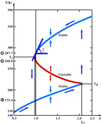
Fig. 1. Bifurcation diagram for the solutions of an energy-balance
model (EBM). Annual mean temperature T vs. fractional change of insolation at the top of the atmosphere µ. The arrows pointing up and down at about µ = 1.4 indicate the stability of the branches: towards a given branch if it is stable and away if it is unstable. The other arrows show the hysteresis cycle that global temperatures would have to undergo for a transition from the upper stable branch to the lower one and back. The angle γ gives the measure of the present climate’s sensitivity to changes in insolation (after Ghil and Childress, 1987).
Here Ri and Ro are incoming solar radiation and outgoing terrestrial radiation. The heat capacity c is that of the global atmosphere, plus that of the global ocean or some fraction thereof, depending on the time scale of interest: one might include only in c the ocean mixed layer when interested in subannual time scales, but the entire ocean could be included in c when studying paleoclimate. The rate of change of T with time t is given by dT /dt, while Q0is the solar
radia-tion received at the top of the atmosphere, σ is the Stefan-Boltzmann constant, and µ is an insolation parameter, equal to unity for present-day conditions. To have a closed, self-consistent model, the planetary reflectivity or albedo α and greyness factor m have to be expressed as functions of T ; m =1 for a perfectly black body and 0 < M < 1 for a grey body, such as planet Earth.
There are two kinds of one-dimensional (1-D) atmospheric models, for which the single spatial variable is latitude or height, respectively. The former are so-called energy-balance models (EBMs: Budyko, 1969; Sellers, 1969) which con-sider the generalization of the model (2.1) for the evolution
of surface-air temperature T = T (x, t ), for example, c(x)∂T
∂t =Ri −Ro+D. (2.2)
Here the terms on the right-hand side can be functions of the meridional coordinate x (latitude, co-latitude, or sine of latitude), as well as of time t , and temperature T . The hor-izontal heat-flux term D expresses heat exchange between latitude belts; it typically contains first and second partial derivatives of T with respect to x. Hence, the rate of change of local temperature T with respect to time also becomes a partial derivative, ∂T /∂t .
The first striking results of theoretical climate dynamics were obtained in showing that slightly different forms of Eq. (2.2) could have two stable steady-state solutions, de-pending on the value of the insolation parameter µ (see Eq. (2.1b)) (Held and Suarez, 1974; Ghil, 1976; North et al., 1981). This multiplicity of stable steady states or physically possible “climates” of our planet can be explained in its sim-plest form in the 0-D model (2.1). This simple explanation resides in the fact that for a fairly broad range of µ-values around µ = 1.0 the curves for Ri and Roas a function of T intersect in 3 points. One of these corresponds to the present climate (highest T -value), and another one corresponds to an ice-covered planet (lowest T -value); both of these are stable, while the third one (intermediate T -value) is unstable. To obtain this result, it suffices to assume that α = α(T ) is a piecewise-linear function of T , with high albedo at low tem-perature, due to the presence of snow and ice, and low albedo at high T , due to their absence, while m = m(T ) is a smooth, increasing function of T that attempts to capture in its sim-plest form the “greenhouse effect” of trace gases and water vapor (Ghil and Childress, 1987, Ch. 10).
The bifurcation diagram of such a 1-D EBM is shown in Fig. 1. It displays the model’s mean temperature T as a func-tion of the fracfunc-tional change µ in the insolafunc-tion Q at the top of the atmosphere. The ‘S’-shaped curve in the figure arises from two back-to-back saddle-node bifurcations. The normal form of the first such bifurcation is
˙
X = µ − X2. (2.3a)
Here X stands for a suitably normalized form of T and ˙X ≡ dX/dtis the rate of change of X, while µ is a parameter that measures the stress on the system, in particular, a normalized form of the insolation parameter.
The upper-most branch corresponds to the steady-state so-lution X = +√µ of Eq. (2.3a) and is stable. It matches rather well the Earth’s present-day climate for µ = 1.0, more precisely, the steady-state solution T = T (x; µ) of the full 1-D EBM (not shown) matches closely the annual mean tem-perature profile from instrumental data over the last century (Ghil, 1976).
The intermediate branch starts out at the left as the second solution, X = −√µ, of Eq. (2.3a) and is unstable. It blends smoothly into the upper branch of a coordinate-shifted and mirror-reflected version of (2.3a), for example,
˙
This branch, X = Xo+
√
µ0−µ, is also unstable.
Finally, the lowermost branch in Fig. 1 is the second steady-state solution of Eq. (2.3b), X = Xo−
√ µ0−µ,
and it is also stable. It corresponds to an ice-covered planet the same distance from the Sun as the Earth.
The fact that the upper-left bifurcation point in Fig. 1 is so close to present-day insolation values created great con-cern in the climate dynamics community in the mid-1970s, when these results were first obtained. Indeed, much more detailed computations (see Sect. 2.3 below) confirmed that a reduction of about 2–5% of insolation values would suf-fice to precipitate Earth into a “deep freeze” (Wetherald and Manabe, 1975). The great distance of the lower-right bifur-cation point from present-day insolation values, on the other hand, suggests that one would have to nearly double atmo-spheric opacity for the the Earth’s climate to jump back to more comfortable temperatures.
2.3 Other atmospheric processes and models
The 1-D atmospheric models in which the details of radia-tive equilibrium are investigated with respect to a height coordinate z (geometric height, pressure, etc.) are often called radiative-convective models (Manabe and Strickler, 1964; Ramanathan and Coakley, 1978; Charlock and Sell-ers, 1980). This name emphasizes the key role that convec-tion plays in vertical heat transfer. While these models pre-ceded historically EBMs as rungs on the modeling hierarchy, it was only recently shown that they too can exhibit multi-ple equilibria (Li et al., 1997; Renn´o, 1997; Ide et al., 2001). The word (stable) “equilibrium,” here and in the rest of this paper, refers simply to a (stable) steady-state of the model, rather than to true a thermodynamic equilibrium.
Two-dimensional (2-D) atmospheric models also have two types according to the third space coordinate which is not ex-plicitly included. Models that resolve exex-plicitly two horizon-tal coordinates on the sphere or on a plane tangent to it tend to emphasize the study of the dynamics of large-scale atmo-spheric motions (see Sec. II in Ghil and Robertson, 2000). They often have a single layer (Charney and DeVore, 1979; Legras and Ghil, 1985) or two (Lorenz, 1963b; Reinhold and Pierrehumbert, 1982). Those that resolve explicitly a merid-ional coordinate and height are essentially combinations of EBMs and radiative-convective models and emphasize there-with the thermodynamic state of the system, rather than its dynamics (Saltzman and Vernekar, 1972; MacCracken and Ghan, 1988; Gall´ee et al., 1991; Berger et al., 1998).
Yet another class of “horizontal” 2-D models is the exten-sion of EBMs to resolve zonal, as well as meridional surface features, in particular, land-sea contrasts (Adem, 1970; North et al., 1983; Chen and Ghil, 1996). We shall see in Sect. 3.2 how such a 2-D EBM is used, when coupled to an oceanic model, to help solve Problem 5.
Additional types of 1-D and 2-D atmospheric models are discussed and references to these and to the types discussed above are given by Schneider and Dickinson (1974) and by Ghil and Robertson (2000), along with some of their main
applications. Finally, to encompass and resolve the main at-mospheric phenomena with respect to all three spatial coor-dinates, general circulation models (GCMs) occupy the pin-nacle of the modeling hierarchy (Randall, 2000).
Ghil and Robertson (2000) also describe the separate hi-erarchies that have grown over the last quarter of a century in modeling the ocean, and the coupled ocean-atmosphere system. More recently, an overarching hierarchy of Earth-system models that encompass all the subEarth-systems of interest (atmosphere, biosphere, cryosphere, hydrosphere and litho-sphere) has been developing. Eventually, the partial results about each subsystem’s variability, as outlined in this section and the next one, will have to be verified from one rung to the next of the Earth-system modeling hierarchy. No reliable solution to Problem 10 is conceivable, at least at the present time, without the full use of such a hierarchy.
2.4 Climate sensitivity
The results of climate simulations with GCMs, whether at-mospheric or coupled, are often interpreted in terms of the understanding gained from 0-D or 1-D EBMs. Wetherald and Manabe (1975), using a simplified sectorial GCM, con-firmed the dependence of mean zonal temperature on the in-solation parameter µ (the normalized “solar constant”) ob-tained for 1-D EBMs (see Ghil and Childress, 1987, Ch. 10). These authors could not confirm the presence of the interme-diate, unstable branch or of the “deep-freeze” stable branch in Fig. 1 with their GCM, due to the model’s computational limitations. But the parabolic shape of the upper, present-daylike branch near the upper-left bifurcation point in our figure (Eq. 2.3a) was well supported by their GCM simula-tions.
In fact, the sensitivity tan γ = (dT /dµ)|µ=1.0 of global
temperature T to changes in µ near the present-day climate (see Fig. 1) equals about 1K per 1% change in the insolation for both EBMs and GCMs. Many studies of climate-change response to increases in greenhouse trace-gas concentrations use, therefore, a linearized version of Eq. (2.1),
cdT dt = −λT + Q, (2.4a) λ = l X i=1 λi, Q = J X j =1 Qj, (2.4b, c)
to interpret the results of detailed GCM simulations. Such interpretations focus on the roles of the different feedbacks λi, positive (λi <0) or negative (λi >0), and heat sources, Qj > 0, or sinks, Qj < 0 (e.g. Schlesinger and Mitchell, 1987; Cess, et al., 1989; Li and Le Treut, 1992). These interpretations are limited, therefore, to equilibrium or quasi-equilibrium responses. The complete study of the hu-man effects on changes in climatic variability requires the use of models that reproduce natural variations in a satisfac-tory manner, rather than simulating only equilibria and sim-ple transients (Ghil and Le Treut, 1999). We proceed,
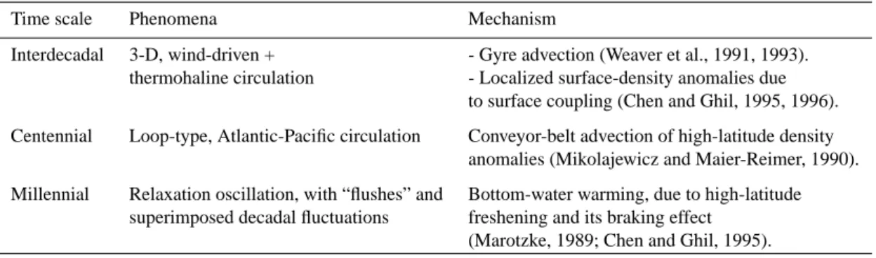
there-Table 1. Thermohaline circulation (THC) oscillations (adapted from Ghil, 1994)
Time scale Phenomena Mechanism
Interdecadal 3-D, wind-driven + - Gyre advection (Weaver et al., 1991, 1993). thermohaline circulation - Localized surface-density anomalies due
to surface coupling (Chen and Ghil, 1995, 1996). Centennial Loop-type, Atlantic-Pacific circulation Conveyor-belt advection of high-latitude density
anomalies (Mikolajewicz and Maier-Reimer, 1990). Millennial Relaxation oscillation, with “flushes” and Bottom-water warming, due to high-latitude
superimposed decadal fluctuations freshening and its braking effect (Marotzke, 1989; Chen and Ghil, 1995).
fore, with a description of internal variability that arises in the context of solving Problem 5.
3 Interdecadal oscillations in the oceans’ thermohaline circulation
3.1 Theory and simple models
Historically, the thermohaline circulation (THC) was first among the climate system’s major processes to be studied using a very simple mathematical model. Stommel (1961) formulated a two-box model and showed that it possessed multiple equilibria.
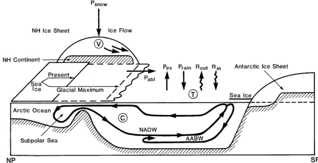
A sketch of the Atlantic Ocean’s THC and its interactions with the atmosphere and cryosphere on long time scales is shown in Fig. 2. These interactions can lead to climate os-cillations with multi-millennial periods, such as the Hein-rich events (Ghil, 1994, and references therein), and are summarized in the figure’s caption, following Ghil et al. (1987). An equally schematic view of the global THC is provided by the widely known “conveyor belt” diagram (e.g. Broecker, 1991). The latter diagram does not commonly in-clude the THC’s interactions with water in its gaseous and solid phases, which our figure does include.
Basically, the THC is due to denser water sinking, lighter water rising, and water-mass continuity closing the circuit through near-horizontal flow between the areas of rising and sinking. This is roughly the oceanic equivalent of the atmo-sphere’s Hadley circulation, with two notable differences:
i) The ocean water’s density ρ is a function of tempera-ture T and salinity S, while that of the air depends on temperature and humidity.
ii) Water sinks in and near fairly concentrated regions of intense convection, currently located primarily in high latitudes, and rises diffusely over the rest of the ocean. Air, on the other hand, does rise most intensely in cu-mulus towers, but overall, the areas of net rising and sinking air in a Hadley cell are quite comparable in ex-tent when viewed on the synoptic and planetary scales. The effects of temperature and salinity on the ocean wa-ter’s density, ρ = ρ(T , S), oppose each other: the density
ρdecreases with increasing T and increases with increasing S. It is these two effects that give the thermohaline circula-tion its name, from the Greek words for T and S. In high latitudes, ρ increases as the water loses heat to the air above and, if sea ice is formed, as the water underneath is enriched in brine. In low latitudes, ρ increases due to evaporation but decreases due to heat flux in the ocean.
For the present climate, the temperature effect is com-monly assumed to be stronger than the salinity effect. Ocean water is observed to sink in certain areas of the high-latitude North Atlantic and Southern Oceans, with very few, limited areas of deep-water formation elsewhere, and to rise every-where else. Thus, the adjective “thermohaline” indicates that T is more important than S by placing “thermo” before “ha-line”. During some remote geological times, deep water may have formed in the global ocean near the equator; such an overturning circulation of the opposite sign to that prevail-ing today has been dubbed halothermal, S before T (e.g. Kennett and Stott, 1991; see, however, Bice and Marotzke, 2001). The quantification of the relative effects of T and S on the oceanic water masses’ buoyancy in high and low lat-itudes is far from complete, especially for paleocirculations; the association of the latter with salinity effects that exceed the thermal ones is thus rather tentative.
Stommel (1961) considered a two-box model, with two pipes connecting the two boxes. He showed that the sys-tem of two nonlinear, coupled ordinary differential equa-tions (ODEs), which govern the temperature and salinity dif-ferences between the two well-mixed boxes has two stable steady-state solutions, distinguished by the direction of flow in the upper and lower pipe. Stommel’s paper was primarily concerned with distinct local convection regimes, and hence vertical stratifications, for example, in the North Atlantic and Mediterranean (or Red Sea). Today, we primarily think of one box as representing the low latitudes and the other one as representing the high latitudes in the global THC.
The next step in the hierarchical modeling of the THC is that of 2-D meridional plane models (see Sect. I.B of Ghil and Robertson, 2000), in which the temperature and salin-ity fields are governed by coupled nonlinear partial differ-ential equations with two independent space variables, for example, latitude and depth. Given boundary conditions for
Fig. 2. Diagram of an Atlantic meridional cross section from North Pole (NP) to South Pole (SP), showing mechanisms likely to affect the
thermohaline circulation (THC) on various time scales. Changes in the radiation balance Rin−Routare due, at least in part, to changes in
the extent of the northern hemisphere (NH) snow and ice cover, V , and how they affect the global temperature, T ; the extent of the southern hemisphere ice is assumed constant, to a first approximation. The change in hydrologic cycle expressed in the terms Prain−Pevapfor the
ocean and Psnow−Pablfor the snow and ice is due to changes in ocean temperature. Deep-water formation in the North Atlantic Subpolar
Sea (North Atlantic Deep Water: NADW) is affected by changes in ice volume and extent, and regulates the intensity C of the THC; changes in Antarctic Bottom Water (AABW) formation are neglected in this approximation. This, in turn, affects the system’s temperature, and is also affected by it (after Ghil et al., 1987).
such a model that are symmetric about the equator, as are the equations themselves, one expects a symmetric solution in which water either sinks near the poles and rises everywhere else (thermohaline), or sinks near the equator and rises ev-erywhere else (halothermal). These two symmetric solutions would correspond to the two equilibria of Stommel’s (1961) box model.
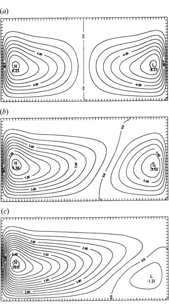
In fact, Fig. 3 shows that symmetry breaking can oc-cur, leading gradually from a symmetric two-cell circulation (Fig. 3a) to an antisymmetric one-cell circulation (approxi-mately achieved in Fig. 3c). In between, all degrees of dom-inance of one cell over the other are possible, with one such intermediate state shown in Fig. 3b. A situation lying some-where between Figs. 3b and c seems to resemble most closely the meridional overturning diagram of the Atlantic Ocean in Fig. 2.
This symmetry breaking can be described by a pitchfork bifurcation (e.g. Guckenheimer and Holmes, 1983):
˙
X = µ − X3. (3.1)
Here X stands for the amount of asymmetry in the solution, so that X = 0 is the symmetric branch, and µ is a parameter that measures the stress on the system, in particular, a nor-malized form of the buoyancy flux at the surface. For µ < 0 the symmetric branch is stable, while for µ > 0, the two branches X = ±√µinherit its stability.
Thus, Figs. 3b and c both lie on a solution branch of the 2-D THC problem for which the left cell dominates, i.e. North
Atlantic Deep Water extends to the Southern Ocean’s po-lar front, as it does in Fig. 2. According to Eq. (3.1), an-other branch exists whose flow patterns are mirror images in the rectangular box’s vertical symmetry axis (the “equa-torial plane”) of those in Figs. 3b and c. The existence of this second branch was verified numerically by Quon and Ghil (1992; their Fig. 16). Thual and McWilliams (1992) considered more complex bifurcation diagrams for a similar 2-D model and showed the equivalence of such a diagram for their 2-D model and a box-and-pipe model of sufficient complexity (see also Dijkstra and Ghil, 2001).
3.2 Bifurcation diagrams for GCMs
Bryan (1986) was the first to document the transition from a two-cell to a one-cell circulation in a simplified ocean GCM with idealized, symmetric forcing, in agreement with the three-box scenario of Rooth (1982). Manabe and Stouf-fer (1999), among others, questioned, however, the realism of more than one stable THC equilibrium by using coupled ocean-atmosphere GCMs. The situation with respect to the THC’s pitchfork bifurcation (3.1) is thus subtler than it was with respect to Fig. 1 for radiative equilibrium. In Sect. 2, atmospheric GCMs confirmed essentially the EBM results. Climbing the rungs of the modeling hierarchy for the THC, however, yields contradictory results that are still in need of further clarification.
reg-Fig. 3. Stream-function fields for a 2-D, meridional plane THC
model with so-called mixed boundary conditions: the temperature profile and salinity flux are imposed at one horizontal boundary of the rectangular box, while the other three boundaries are imper-meable to heat and salt. (a) Symmetric solution for low salt-flux forcing; (b, c) increasingly asymmetric solutions as the forcing is increased (from Quon and Ghil, 1992).
ular excursions than the huge and completely irregular jumps associated with bistability, was studied intensively in the late 1980s and the 1990s. These studies placed themselves on various rungs of the modeling hierarchy, from Boolean de-lay equation models (so-called “formal conceptual models”: Ghil et al., 1987; Darby and Mysak, 1993) through box mod-els (Welander, 1986) and 2-D modmod-els (Quon and Ghil, 1995) to ocean GCMs. A summary of the different kinds of os-cillatory variability found in the latter appears in Table 1. Additional GCM references for these three types of oscil-lations are given by McWilliams (1996). Such oscillatory behaviour seems to match more closely the instrumentally recorded THC variability (see Sect. 3.3 below), as well as
the paleoclimatic records for the recent geological past (see Ghil, 1994), than bistability.
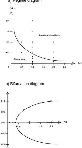
The interaction of the (multi-)millennial oscillations with variability in the surface features and processes shown in Fig. 2 is discussed by Ghil (1994). Chen and Ghil (1996), in particular, studied some of the interactions between atmo-spheric processes and the THC. They used a so-called hy-brid coupled model to depict a (horizontally) 2-D EBM (see Sect. 2.3) coupled to a rectangular-box version of the North Atlantic rendered by a low-resolution ocean GCM. This hy-brid model’s regime diagram is shown in Fig. 4a. A steady state is stable for high values of the coupling parameter λao or of the EBM’s diffusion parameter d. Interdecadal oscil-lations with a period of 40–50 years are self-sustained and stable for low values of these parameters.
The self-sustained THC oscillations in question are char-acterized by a pair of vortices of opposite sign that grow and decay in quadrature with each other in the ocean’s up-per layers. Their centers follow each other counterclockwise through the northwestern quadrant of the model’s rectangular domain. Both the period and the spatio-temporal character-istics of the oscillation are thus rather similar to those seen in a fully coupled GCM with realistic geometry (Delworth et al., 1993).
The transition from a stable equilibrium to a stable limit cycle, via Hopf bifurcation, in Chen and Ghil’s hybrid cou-pled model is shown in Fig. 4b. The physical characteris-tics of the oscillatory instability that leads to the Hopf bi-furcations have been described in further detail by Colin de Verdi`ere and Huck (1999), using both a four-box ocean-atmosphere and a number of more detailed models.
3.3 Interannual and interdecadal climate variability Human intervention in the workings of the climate on the global scale (Problem 9) is most likely to occur on time scales comparable to those of major socio-economic changes. The latter typically take place at this turn of the century on interannual to interdecadal time scales. The so-lution to Problem 9 is thus clearly predicated, at least, on satisfactory solutions to Problems 3 and 5.
The best known climatic regularities on the interan-nual time scale are the quasi-biennial and low-frequency (4–5-year) component of the El-Ni˜no/Southern-Oscillation (ENSO) phenomenon (Rasmusson et al., 1990; Neelin et al., 1998). A particularly appealing explanation of these two spectral peaks that also allows for the broadband spectrum in the 1–10-year band is given by the Devil’s staircase mech-anism (Jin et al., 1994, 1996; Tziperman et al., 1994; Saun-ders and Ghil, 2001). This broadband spectral background is consistent with the occurrence of major warm events in the tropical Pacific every 2–7 years.
This mechanism is most easily explained in two steps. First, it is by now well accepted that the coupled ocean-atmosphere system in the tropical Pacific exhibits a self-sustained oscillation with a period of 2–3 years for mean-annual conditions. Second, this self-sustained oscillation
in-teracts with the seasonal cycle in insolation and it frequency-locks, preferentially to an integer multiple of the forcing pe-riod: 2, 3, 4 or 5 years. Jumps between these broad inte-ger steps in the Devil’s staircase, as well as between nar-rower steps associated with rational periods, such as 4/3 years (≈ 16 months), occur as the result of atmospheric, higher-frequency “noise.” This mechanism is described fur-ther and compared with ofur-ther scenarios of interannual vari-ability and with the observational evidence in Sec. III of Ghil and Robertson (2000); see also Ch. 5 of Dijkstra (2000).
A fairly satisfactory, albeit partial, solution to Problem 3 is thus at hand, insofar as we understand ENSO’s spectral regularities. No complete consensus has been achieved, how-ever, as yet, on the relative role of weather noise and coupled-mode nonlinearities in ENSO’s irregularity, i.e. the irregular occurrence of major warm events.
Ghil and Vautard (1991) described statistically significant regularities in the interdecadal band of climatic variability. Broad peaks of roughly 13–15 and 23–27 years have been since confirmed in various records, both instrumental (Plaut et al., 1995; Moron et al., 1998) and paleoclimatic. The evi-dence for these interdecadal peaks is reviewed by Ghil et al. (2001). The interdecadal oscillations in the THC reviewed in Sect. 3.2 above are a plausible mechanism for these peaks, but not yet generally accepted as such. We are thus making good progress on Problem 5, but do not expect a fully self-consistent solution in less than 2-3 decades.
4 Concluding remarks
We have cast a bird’s-eye view on selected problems among the ten formulated in the Abstract. This view has clearly em-phasized strong interconnections between them, both pair-wise and all around. Unified methods of solution are pro-vided by dynamical systems theory. Each problem requires the use of a model hierarchy for its solution.
To conclude, we briefly address Problem 9. More pre-cisely, we ask whether the impact of human activities on the climate is observable and identifiable in the instrumental records of the last century-and-a-half and in recent paleocli-mate records? The answer to this question depends on the null hypothesis against which such an impact is tested.
The current approach that is generally pursued assumes essentially that past climate variability is indistinguishable from a stochastic red-noise process (Hasselmann, 1976), whose only regularities are those of periodic external forcing (Mitchell, 1976). Given such a null hypothesis, the official consensus of IPCC (1995) tilts towards a global warming ef-fect of recent trace-gas emissions, which exceeds the cooling effect of anthropogenic aerosol emissions.
Atmospheric and coupled GCM simulations of the trace-gas warming and aerosol cooling buttress this IPCC consen-sus. The GCM simulations used so far do not, however, ex-hibit the observed interdecadal regularities described at the end of Sect. 3.3. They might, therewith, miss some important physical mechanisms of climate variability and are,
there-a) Regime diagram
b) Bifurcation diagram
Fig. 4. Dependence of THC solutions on two parameters in a hybrid
coupled model (HCM); the two parameters are the atmosphereo-cean coupling coefficient λaoand the atmospheric thermal diffusion
coefficient d. (a) Schematic regime diagram. The full circles stand for the model’s stable steady-states, the open circles for stable limit cycles, and the solid curve is the estimated neutral stability curve between the former and the latter. (b) Hopf bifurcation curve at fixed d = 1.0 and varying λao; this curve was obtained by fitting a
parabola to the model’s numerical-simulation results, shown as full and open circles (from Chen and Ghil, 1996).
fore, not entirely conclusive.
As northern hemisphere temperatures were falling in the 1960s and early 1970s, the aerosol effect was the one that caused the greatest concern. As shown in Sect. 2.2, this concern was bolstered by the possibility of a huge, highly nonlinear temperature drop if the climate system reached the upper-left bifurcation point of Fig. 1.
The global temperature increase through the 1990s is cer-tainly rather unusual in terms of the instrumental record of
the last 150 years or so. It does not correspond, however, to a rapidly accelerating increase in greenhouse-gas emissions or a substantial drop in aerosol emissions. How statistically significant is, therefore, this temperature rise, if the null hy-pothesis is not a random coincidence of small, stochastic ex-cursions of global temperatures with all, or nearly all, the same sign?
The presence of internally arising regularities in the cli-mate system with periods of years and decades suggests the need for a different null hypothesis. Essentially, one needs to show that the behaviour of the climatic signal is distinct from that generated by natural climate variability in the past, when human effects were negligible, at least on the global scale. As discussed in Sects. 2.1 and 3.3, this natural vari-ability includes interannual and interdecadal cycles, as well as the broadband component. These cycles are far from be-ing purely periodic. Still, they include much more persistent excursions of one sign, whether positive or negative in global or hemispheric temperatures, say, than does red noise.
Ghil and Jiang (1998) showed that on the seasonal-to-interannual time scale, climate predictability is greatly en-hanced by the presence of these regularities. This is the case not only when the predictability is measured against the clas-sical benchmark of a red-noise process of first-order auto-regressive type (Hasselmann, 1976; Mitchell, 1976; IPCC, 1995). It is also the case when measured against a purely chaotic, albeit deterministic process, such as that governed by Lorenz’s (1963a) model.
The answer to the global warming problem on the inter-decadal time scale on which we are posing this problem is comprised of two parts. First, we need to describe and un-derstand climate variability on this time scale as well as on the interannual time scale, in particular its regularities, i.e. solve Problems 3 and 5. Once that is done, a prediction with known error bars on the interdecadal time scale will be pos-sible (see Plaut et al., 1995).
With these results in hand, we should be able to proceed to the second part of the answer. Can we identify with measur-able certainty deviations of the current record from predic-tions based on past natural variability? If so, such deviapredic-tions have to be attributed to new causes. The “suspects” clearly include human effects, and attribution to them will become thereby both easier and more reliable.
At the same time, one hopes that the applications of dy-namical systems theory to the global socio-economic sys-tem and to population dynamics will have made considerable progress (Keilis-Borok and S´anchez Sorondo, 2000). With this in mind, a rational approach to predicting and controlling the coupled system formed by all living beings on this planet and their physico-chemical environment would become fea-sible by the end of this century.
Acknowledgements. It is a pleasure to thank all the students and
colleagues from whom I learned about dynamical systems theory and its applications to atmospheric, oceanic and climate dynam-ics. Peter Read’s encouragement and insistence as Guest Editor of this Special Issue were of the essence in leading to a finished
product in a timely manner. Eli Tziperman’s comments on the original manuscript have improved the presentation considerably. I am grateful for the sabbatical hospitality of the Ecole Normale Sup´erieure in Paris and its D´epartement Terre-Atmosph`ere-Oc´ean, as well as to the Laboratoire de M´et´eorologie Dynamique du Centre National de la Recherche Scientifique (CNRS) at the Ecole. Their hospitality allowed me to prepare this invited address for the Special Session on Achievements and Directions in Nonlinear Geophysics at the XXVth General Assembly of the European Geophysical So-ciety in Nice, France, 25–29 April 2000. Help with the figures by J. Meyerson and with the text by E. Ridgnal and S. Hernandez is much appreciated. My work on the topics reviewed here has been supported by an NSF Special Creativity Award and by NSF Grant ATM-0082131. This is publication no. 5590 of UCLA’s Institute of Geophysics and Planetary Physics.
References
Adem, J., Incorporation of advection of heat by mean winds and by ocean currents in a thermodynamic model for long-range weather prediction, Mon. Weather Rev., 98, 776–786, 1970.
Arnol’d, V. I., Geometrical Methods in the Theory of Or-dinary Differential Equations, Springer-Verlag, New York/Heidelberg/Berlin, 334, 1983.
Berger A., Loutre, M. F., and Gall´ee, H., Sensitivity of the LLN climate model to the astronomical and CO2 forcings over the last 200 kyr, Clim. Dyn., 14, 615–629, 1998.
Bice, K. L. and Marotzke, J., Numerical evidence against reversed thermohaline circulation in the warm Paleocene/Eocene ocean, J. Geophys. Res., in press, 2001.
Bryan, F., High-latitude salinity effects and interhemispheric ther-mohaline circulations, Nature, 323, 301–304, 1986.
Broecker, W. S., Peteet, D. M., and Rind, D., Does the ocean-atmosphere system have more than one stable mode of opera-tion? Nature, 315, 21–25, 1985.
Broecker, W. S., The great ocean conveyor, Oceanography, 4, 79-89, 1991.
Browder, F. (Ed.), Mathematical Developments Arising from Hilbert’s Problems, American Mathematical Society, Provi-dence, R. I., 1976.
Budyko, M. I., The effect of solar radiation variations on the climate of the Earth, Tellus, 21, 611–619, 1969.
Cess, R. D., Potter, G. L., Blanchet, J. P., Boer, G. J., Ghan, S. J., Kiehl, J. T., Le Treut, H., Li, Z.-X., Liang, X.-Z., Mitchell, J. F. B., Morcrette, J.-J., Randall, D. A., Riches, M. R., Roeckner, E., Schlese, U., Slingo, A., Taylor, K. E., Washington. W. M., Wetherald, R. T., and Yagai, I., Interpretation of cloud-climate feedbacks as produced by 14 atmospheric general circulation models, Science, 245, 513–551, 1989.
Charlock, T. and Sellers, W. D., Aerosol effects on climate: Calculations with time-dependent and steady-state radiative-convective models, J. Atmos. Sci., 37, 1327–1341, 1980. Charney, J. G. and DeVore, J. G., Multiple flow equilibria in the
atmosphere and blocking, J. Atmos. Sci., 36, 1205–1216, 1979. Chen, F. and Ghil, M., Interdecadal variability of the thermohaline
circulation and high-latitude surface fluxes, J. Phys. Oceanogr., 25, 2547–2568, 1995.
Chen, F. and Ghil, M., Interdecadal variability in a hybrid coupled ocean-atmosphere model, J. Phys. Oceanogr., 26, 1561–1578, 1996.
An oceanic wavemaker for interdecadal variability, J. Phys. Oceanogr., 29, 893–910, 1999.
Corry, L., Hilbert and the axiomatization of physics (1894–1905), Arch. History Exact Sciences, 51, 1997.
Crafoord, C. and K¨allen, E., A note on the condition for existence of more than one steady- state solution in Budyko-Sellers type models, J. Atmos. Sci., 35, 1123–1125, 1978.
Darby M. S. and Mysak, L. A., A Boolean delay equation model of an interdecadal Arctic climate cycle, Clim. Dyn., 8, 241–246, 1993.
Delworth, T., Manabe, S., and Stouffer, R. J., Interdecadal vari-ations of the thermohaline circulation in a coupled oceanatmo-sphere model, J. Climate, 6, 1993–2011, 1993.
Dijkstra, H., 2000, Nonlinear Physical Oceanography, Kluwer Acad. Publishers, Dordrecht/ Norwell, Mass., 456, 2000. Dijkstra, H. and Ghil, M., Low-frequency variability of the
large-scale ocean circulation: A dynamical systems approach, Rev. Geophys., submitted, 2001.
Eckmann, J.-P. and Ruelle, D., Ergodic theory of chaos and strange attractors, Rev. Mod. Phys., 57, 617–656, 1985, addendum, Rev. Mod. Phys., 57, 1115, 1985
Gall´ee, H., van Ypersele, J. P., Fichefet, Th., Tricot, C., and Berger, A., Simulation of the last glacial cycle by a coupled, sectorially averaged climateice-sheet model. I. The climate model, J. Geo-phys. Res., 96, 13, 139–161, 1991.
Ghil, M., Climate stability for a Sellers-type model, J. Atmos. Sci., 33, 3–20, 1976.
Ghil, M., Cryothermodynamics: The chaotic dynamics of paleocli-mate, Physica D, 77, 130–159, 1994.
Ghil, M. and Le Treut, H., A climate model with cryodynamics and geodynamics, J. Geophys. Res., 86, 5262–5270, 1981.
Ghil, M. and Childress, S., Topics in Geophysical Fluid Dynamics: Atmospheric Dynamics, Dynamo Theory and Climate Dynam-ics, Springer-Verlag, New York/Berlin/London/ Paris/Tokyo, 485, 1987.
Ghil, M. and Vautard, R., Interdecadal oscillations and the warming trend in global temperature time series, Nature, 350, 324–327, 1991.
Ghil, M. and Jiang, N., Recent forecast skill for the El-Ni˜no/Southern Oscillation, Geophys. Res. Lett., 25, 171–174, 1998.
Ghil, M. and Le Treut, H., Climate variability and climate change, in Scientific Bridges for 2000 and Beyond, a Virtual Collo-quium by the Elf-Aquitaine Professors of the Acad´emie des Sci-ences, Rapports de l’Acad´emie des SciSci-ences, TEC & DOC, Lon-don/Paris/NewYork, 105–119, 1999.
Ghil, M. and Robertson, A. W., Solving problems with GCMs: General circulation models and their role in the climate model-ing hierarchy, in General Circulation Model Development: Past, Present and Future, D. Randall (Ed.), Academic Press, San Diego, 285–325, 2000.
Ghil, M., Benzi, R., and Parisi, G. (Eds.), Turbulence and Pre-dictability in Geophysical Fluid Dynamics and Climate Dynam-ics, North-Holland, Amsterdam/NewYork/Oxford/Tokyo, 449, 1985.
Ghil, M., Mullhaupt, A., and Pestiaux, P., Deep water formation and Quaternary glaciations, Climate Dyn., 2, 1–10, 1987.
Ghil, M., Kimoto, M., and Neelin, J. D., Nonlinear dynamics and predictability in the atmospheric sciences, Rev. Geophys., Sup-plement (U.S. Nat’l Rept. to Int’l Union of Geodesy & Geophys. 1987–1990), 29, 46–55, 1991.
Ghil, M., Allen, M. R., Dettinger, M. D., Ide, K., Kondrashov, D.,
Mann, M. E., Robertson, A. W., Saunders, A., Tian, Y., Varadi, F., and Yiou, P., Advanced spectral methods for climatic time series, Rev. Geophys., accepted, 2001.
G¨odel, K., The Consistency of the Axiom of Choice and of the Gen-eralized Continuum Hypothesis, Princeton Univ. Press, Prince-ton, 1940.
Guckenheimer, J. and Holmes, P., Nonlinear Oscillations, Dynam-ical Systems and Bifurcations of Vector Fields, Springer-Verlag, New York, 453, 1983.
Hasselmann, K., Stochastic climate models, Part I: Theory. Tellus, 28, 473–485, 1976.
Held, I. M. and Suarez, M. J., Simple albedo feedback models of the ice caps, Tellus, 26, 613–629, 1974.
Hilbert, D., Mathematische Probleme, G¨ottinger Nachrichten, [see also Archiv d. Mathematik u. Physik, 3 (1), 44–63 and 213–237, 1901; French transl. by M. L. Laugel, Sur les probl`emes futurs des math´ematiques in Comptes Rendus du 2´eme Congr`es In-ternational des Math´ematiciens, 58–114, Gauthier-Villars, Paris, 1902; Engl. transl. by M. Winton Newson, Bull. Amer. Math. Soc., 8, 437–479, 1902], 253–297, 1900.
Ide, K., Le Treut, H., Li, Z.-X., and Ghil, M., Atmospheric radia-tive equilibria. Part II: Bimodal solutions for atmospheric optical properties, Climate Dyn., in press, 2001.
IPCC (Intergovernmental Panel on Climate Change), Climate Change 1995: The Science of Global Change, Houghton, J. T., Meira Filho, L. G., Callander, B. A., Harris, N., Kattenberg, A., and Maskell, K., Eds., Cambridge University Press, Cambridge, UK, 572, 1995.
Jiang, S., Jin, F.-F., and Ghil, M., Multiple equilibria, periodic, and aperiodic solutions in a wind-driven, double-gyre, shallow-water model, J. Phys. Oceanogr., 25, 764–786, 1995.
Jin, F.-F., Neelin, J. D., and Ghil, M., El Ni˜no on the Devil’s Stair-case: Annual subharmonic steps to chaos, Science, 264, 70–72, 1994.
Jin, F.-F., Neelin, J. D., and Ghil, M., El Ni˜no/Southern Oscilla-tion and the annual cycle: Subharmonic frequency-locking and aperiodicity, Physica D, 98, 442–465, 1996.
Kaplansky, I., Hilbert’s Problems, Univ. of Chicago Press, Chicago, 1977.
Keilis-Borok, V. I. and S´anchez Sorondo, M., (Eds.), Science for Survival and Sustainable Development, Pontifical Academy of Sciences, Vatican City, 427, 2000.
Kennett, R. P. and Stott, L. D., Abrupt deep-sea warming, paleo-ceanographic changes and benthic extinctions at the end of the Palaeocene, Nature, 353, 225–229, 1991.
Keppenne, C. L., Marcus, S., Kimoto, M. and Ghil, M., Intrasea-sonal variability in a two-layer model and observations, J. Atmos. Sci., 57, 1010–1028, 2000.
Kuhn, T. S., The Structure of Scientific Revolutions, 2nd ed., Univ. of Chicago Press, Chicago/London, 210, 1970.
Legras, B. and Ghil, M., Persistent anomalies, blocking and varia-tions in atmospheric predictability, J. Atmos. Sci., 42, 433–471, 1985.
Li, Z.-X. and Le Treut, H., Cloud-radiation feedbacks in a general circulation model and their dependence on cloud modelling as-sumptions, Clim. Dyn., 7, 133–139, 1992.
Li, Z.-X., Ide, K., LeTreut, H., and Ghil, M., Atmospheric radiative equilibria in a simple column model, Clim. Dyn., 13, 429–440, 1997.
Lorenz, E. N., Deterministic nonperiodic flow, J. Atmos. Sci., 20, 130–141, 1963a.
448–464, 1963b.
Lorenz, E. N., Three approaches to atmospheric predictability, Bull. Amer. Met. Soc., 50, 345–351, 1969.
MacCracken, M. C. and Ghan, S. J., Design and use of zonally av-eraged models in Physically- Based Modeling and Simulation of Climate and Climatic Change, M. E. Schlesinger (Ed.), Kluwer Acad. Publishers, Dordrecht, 755–803, 1988.
Manabe, S. and Strickler, R. F., Thermal equilibrium of the atmo-sphere with a convective adjustment, J. Atmos. Sci., 21, 361– 385, 1964.
Manabe, S. and Stouffer, R. J., Are two modes of thermohaline cir-culation stable? Tellus, 51A, 400–411, 1999.
Marotzke, J., Instabilities and multiple steady states of the ther-mohaline circulation, in Ocean Circulation Models: Combining Data and Dynamics, D. L. T. Anderson and J. Willebrand (Eds.), Kluwer Academic, 501–511, 1989.
Marotzke, J., Welander, P., and Willebrand, J., Instability and multi-ple steady states in a meridional-plane model of the thermohaline circulation, Tellus, 40A, 162–172, 1988.
Martinson, D. G., Bryan, K., Ghil, M., Hall, M. M., Karl, T. R., Sarachik, E. S., Sorooshian, S., and Talley, L. D., Eds., Natural Climate Variability on Decade-to-Century Time Scales, National Academy Press, Washington, D.C., 630, 1995.
McWilliams, J. C., Modeling the oceanic general circulation, Annu. Rev. Fluid. Mech., 28, 215–48, 1996.
Mikolajewicz, U. and Maier-Reimer, E., Internal secular variability in an ocean general circulation model, Clim. Dyn., 4, 145–156, 1990.
Mitchell, J. M., Jr., An overview of climatic variability and its causal mechanisms, Quartern. Res., 6, 481–493, 1976.
Moron, V., Vautard, R., and Ghil, M., Trends, interdecadal and in-terannual oscillations in global sea-surface temperatures, Clim. Dyn., 14, 545–569, 1998.
Neelin, J. D., Battisti, D. S., Hirst, A. C., Jin, F.-F., Wakata, Y., Yas-magata, T., and Zebiak, S. E., ENSO theory, J. Geophys. Res., 103, 14, 261–14, 290, 1998.
North, G. R., Mengel, J. G., and Short, D. A., Simple energy bal-ance model resolving the seasons and the continents: Application to the astronomical theory of the ice ages, J. Geophys. Res., 88, 6576–6586, 1983.
North, G. R., Cahalan, R. F., and Coakley, J. A. Jr., Energy balance climate models, Rev. Geophys. Space Phys., 19, 91–121, 1981. Pfeffer, R. L. (Ed.), Dynamics of Climate, Pergamon Press, New
York/Oxford/London/Paris, 137, 1960.
Plaut, G., Ghil, M., and Vautard, R., Interannual and interdecadal variability in 335 years of Central England temperatures, Sci-ence, 268, 710–713, 1995.
Quon, C. and Ghil, M., Multiple equilibria in thermosolutal convec-tion due to salt-flux boundary condiconvec-tions, J. Fluid Mech., 245, 449–483, 1992.
Quon, C. and Ghil, M., Multiple equilibria and stable oscillations in thermosolutal convection at small aspect ratio, J. Fluid. Mech., 291, 33–56, 1995.
Ramanathan, V. and Coakley, J. A., Climate modeling through ra-diative convective models, Rev. Geophys. Space Phys., 16, 465– 489, 1978.
Randall, D. (Ed.), General Circulation Model Development: Past, Present and Future (Academic Press, San Diego) 803, 2000. Rasmusson, E. M., Wang, X., and Ropelewski, C. F., The biennial
component of ENSO variability, J. Marine Syst., 1, 71–96, 1990. Reid, C., Hilbert, Springer-Verlag, New York/Heidelberg/Berlin,
1970.
Reinhold, B. B. and Pierrehumbert, R. T., Dynamics of weather regimes: Quasi-stationary waves and blocking, Mon. Wea. Rev., 110, 1105–1145, 1982.
Renn´o, N. O., Multiple equilibria in radiative-convective atmo-spheres, Tellus, 49A, 423–438, 1997.
Rooth, C., Hydrology and ocean circulation, Progr. Oceanogr., 11, 131–149, 1982.
Saltzman, B., Paleoclimatic modeling, in Paleoclimate Analysis and Modeling, A. D. Hecht, ed. J. Wiley, New York, 341–396, 1985. Salzman, B. and Vernekar, A. D., Global equilibrium solutions for the zonally averaged macroclimate, J. Geophys. Res., 77, 3936– 3945, 1972.
Saunders, A. and Ghil, M., A Boolean delay equations model of ENSO variability, Physica D, accepted, 2001.
Schlesinger, M. E. and Mitchell, J. B., Climate model simulations of the equilibrium climatic response to increased carbon dioxide., Rev. Geophys., 25, 760–798, 1987.
Schneider, S. H. and Dickinson, R. E., Climate modeling, Rev. Geo-phys. Space Phys., 25, 447–493, 1974.
Sellers, W. D., A climate model based on the energy balance of the earth-atmosphere system, J. Appl. Meteor., 8, 392–400, 1969. Smale, S., Differentiable dynamical systems. Bull. Amer. Math.
Soc., 73, 747–817, 1967.
Speich, S., Dijkstra, H., and Ghil, M., Successive bifurcations in a shallow-water model, applied to the wind-driven ocean circula-tion, Nonlin. Proc. Geophys., 2, 241–268, 1995.
Stommel, H., Thermohaline convection with two stable regimes of flow, Tellus, 13, 224–230, 1961.
Strong, C. M., Jin, F.-F., and Ghil, M., Intraseasonal oscillations in a barotropic model with annual cycle and their predictability, J. Atmos. Sci., 52, 2627–2642, 1995.
Thompson, P. D., Numerical Weather Analysis and Prediction, Macmillan, New York, 170, 1961.
Thual, O. and McWilliams, J. C., The catastrophe structure of ther-mohaline convection in a two-dimensional fluid model and a comparison with low-order box models, Geophys. Astrophys. Fluid Dyn., 64, 67–95, 1992.
Trenberth, K. (Ed.), Climate System Modeling (Cambridge Univer-sity Press, Cambridge/New York) 788, 1992.
Tziperman, E., Stone, L., Cane, M., and Jarosh, H., El Ni˜no chaos: Overlapping of resonances between the seasonal cycle and the Pacific ocean-atmosphere oscillator, Science, 264, 72–74, 1994. Veronis, G., An analysis of wind-driven ocean circulation with a
limited number of Fourier components. J. Atmos. Sci., 20, 577– 593, 1963.
Veronis, G., Wind-driven ocean circulation. Part II. Deep-Sea Res., 13, 30–55, 1966.
Weaver, A. J., Sarachik, E. S., and Marotzke, J., Freshwater flux forcing of decadal and interdecadal oceanic variability, Nature, 353, 836–838, 1991.
Weaver, A. J., Marotzke, J., Cummings, P. F., and Sarachick, E. S., Stability and variability of the thermohaline circulation, J. Phys. Oceanogr., 23, 39–60, 1993.
Welander, P., Thermohaline effects in the ocean circulation and related simple models, in Large-Scale Transport Processes in Oceans and Atmosphere, Willebrand and D. L. T. Anderson (Eds.), D. Reidel, 163–200, 1986.
Wetherald, R. T. and Manabe, S., The effect of changing the solar constant on the climate of a general circulation model, J. Atmos. Sci., 32, 2044–2059, 1975.
Weyl, H., David Hilbert and his mathematical work, Bull. Amer. Math. Soc., 60, 612–654, 1944.