Operational ocean models in the Adriatic Sea: a skill assessment

(1)

HAL Id: hal-00298593

https://hal.archives-ouvertes.fr/hal-00298593

Submitted on 21 Dec 2006

HAL is a multi-disciplinary open access

archive for the deposit and dissemination of sci-entific research documents, whether they are pub-lished or not. The documents may come from teaching and research institutions in France or abroad, or from public or private research centers.

L’archive ouverte pluridisciplinaire HAL, est destinée au dépôt et à la diffusion de documents scientifiques de niveau recherche, publiés ou non, émanant des établissements d’enseignement et de recherche français ou étrangers, des laboratoires publics ou privés.

Operational ocean models in the Adriatic Sea: a skill

assessment

J. Chiggiato, P. Oddo

To cite this version:

J. Chiggiato, P. Oddo. Operational ocean models in the Adriatic Sea: a skill assessment. Ocean Science Discussions, European Geosciences Union, 2006, 3 (6), pp.2087-2116. �hal-00298593�

(2)

OSD

3, 2087–2116, 2006

Operational ocean models in the

Adriatic Sea

J. Chiggiato and P. Oddo

Title Page Abstract Introduction Conclusions References Tables Figures ◭ ◮ ◭ ◮ Back Close

Full Screen / Esc

Printer-friendly Version Interactive Discussion

Ocean Sci. Discuss., 3, 2087–2116, 2006 www.ocean-sci-discuss.net/3/2087/2006/ © Author(s) 2006. This work is licensed under a Creative Commons License.

Ocean Science Discussions

Papers published in Ocean Science Discussions are under open-access review for the journal Ocean Science

Operational ocean models in the Adriatic

Sea: a skill assessment

J. Chiggiato1and P. Oddo2

1

Servizio IdroMeteorologico, ARPA Emilia Romagna, Viale Silvani 6, 40122 Bologna, Italy

2

Istituto Nazionale di Geofisica e Vulcanologia, unit `a funzionale di Climatologia Dinamica, via Donato Creti 12, 40128 Bologna, Italy

Received: 30 November 2006 – Accepted: 8 December 2006 – Published: 21 December 2006 Correspondence to: P. Oddo (oddo@bo.ingv.it)

(3)

OSD

3, 2087–2116, 2006

Adriatic Sea

Full Screen / Esc

EGU Abstract

In the framework of the Mediterranean Forecasting System project (MFS) sub-regional and regional numerical ocean forecasting systems performance are assessed by mean of model-model and model-data comparison. Three different operational systems have been considered in this study: the Adriatic REGional Model (AREG); the AdriaROMS

5

and the Mediterranean Forecasting System general circulation model (MFS model). AREG and AdriaROMS are regional implementations (with some dedicated variations) of POM (Blumberg and Mellor, 1987) and ROMS (Shchepetkin and McWilliams, 2005) respectively, while MFS model is based on OPA (Madec et al., 1998) code. The as-sessment has been done by means of standard scores. The data used for operational

10

systems assessment derive from in-situ and remote sensing measurements. In par-ticular a set of CTDs covering the whole western Adriatic, collected in January 2006, one year of SST from space born sensors and six months of buoy data. This allowed to have a full three-dimensional picture of the operational forecasting systems quality during January 2006 and some preliminary considerations on the temporal fluctuation

15

of scores estimated on surface (or near surface) quantities between summer 2005 and summer 2006. In general, the regional models are found to be colder and fresher than observations. They eventually outperform the large scale model in the shallowest lo-cations, as expected. Results on amplitude and phase errors are also much better in locations shallower than 50 m, while degraded in deeper locations, where the models

20

tend to have a higher homogeneity along the vertical column compared to observa-tions. In a basin-wide overview, the two regional models show some dissimilarities in the local displacement of errors, something suggested by the full three-dimensional picture depicted using CTDs, but also confirmed by the comparison with SSTs. In locations where the regional models are mutually correlated, the aggregated

mean-25

square-error has been found to be lower, which is a useful outcome of having several operational systems in the same region.

(4)

OSD

3, 2087–2116, 2006

Adriatic Sea

Full Screen / Esc

1 Introduction

Ocean physical processes play a crucial role in governing marine dynamics (acoustical, biological and sedimentological). Therefore, operational forecasting physical ocean fields can greatly contribute to the understanding of the functioning of marine sub-systems, as well as providing an efficient support tool for marine environmental

man-5

agement (Oddo et al., 2006; Robinson and Sellschopp, 2001). For several applications like fisheries management, naval operations, shipping, tourism, management of ma-rine resources but also for pure scientific purposes fine resolution ocean forecasts are frequently required for limited regions (Onken et al., 2005).

In the framework of Mediterranean Forecasting System project (MFS, Pinardi et al.,

10

2003) a suite of numerical ocean models has been developed and implemented in the Mediterranean Sea. A large scale, coarse resolution model covering the entire Mediterranean region (MFS model) and a number of embedded high-resolution models in different sub-regional seas compose the modelling system. The basic idea is to use the MFS model in order to produce analysis-forecast at basin scale and provide initial

15

and/or lateral boundary conditions to the sub-regional models.

Obviously numerical models are not perfect and several decisions have to be taken by the scientists during the implementation phase (scale resolution, parameterisations and so on). Separating the scales of interest in the implementation phase (the deci-sion to have specific model for different regions) allow to dedicate particular attention

20

to regionally specific numerical requirements. Since the perfect model does not ex-ist, also the perfect tuning is missing. At the present time, several numerical models exist based on the same physical assumptions, and each single model has its own behaviour. Since model results derive from physical laws warped by numerical dis-cretisation techniques, the possibility to have several numerical models implemented

25

in the same area increases the confidence in model results.

To our knowledge, two regional Operational Ocean Forecasting Systems (hereinafter OOFS) are currently producing daily or weekly forecasts, published on free-access web

(5)

OSD

3, 2087–2116, 2006

Adriatic Sea

Full Screen / Esc

EGU sites, covering the whole Adriatic Sea and with a full three-dimensional

implementa-tion of the core ocean model: the Adriatic REGional forecasting system (AREG) and the Adriatic ROMS implementation (AdriaROMS). The major aims of this work are to asses the performances of these two different regional OOFSs, eventually showing the potential advantages deriving from specific regional implementation and from having

5

more OOFSs in the same area. For completeness, also the large-scale Mediterranean system MFS is included in this analysis, even if to a lesser extent, as a proxy of the relative large scale vs. regional systems performance. The analysis is focussed on the quality of the operational systems, i.e., the agreement between model results and independent observations, therefore using the best model output available (that is,

in-10

cluding analyses). The relative skill to provide accurate short term forecast is left to other investigations.

Due to data availability, the analysis has been limited to temperature and salinity fields.

The operational ocean forecasting systems are presented in Sect. 2. In Sect. 3 the

15

comparison between model results and in situ observation is presented. In Sect. 4 the comparison of model sea surface temperatures with remote sensing (AVHRR) data is given. Finally, in Sect. 5, the conclusions of this work are summarised.

2 Operational ocean models

In this section all the operational forecasting systems considered in the comparison

20

are briefly described. These systems differ in many aspects, such as operational suite, spatial discretisation, physical parameterisations, and numerical weather predic-tion system used as surface boundary condipredic-tion. For enhanced readability, the major differences are also summarized in Table 1.

(6)

OSD

3, 2087–2116, 2006

Adriatic Sea

Full Screen / Esc

2.1 MFS

The MFS model (Tonani et al., 20061), based on the OPA code (Madec et al., 1998), covers the entire Mediterranean Sea with an horizontal resolution of 1/16◦ _{of degree}

and 72 unevenly spaced z-coordinate on the vertical. The model is forced at surface with European Centre for Medium range Weather Forecast (ECMWF) analysis and

5

forecast atmospheric fields. It uses a reduced order optimal interpolation assimilation scheme (SOFA, De Mey and Benkiran, 2002; Demirov et al., 2003; Dobricic et al., 2006) to correct the model solution using vertical profiles from XBT and ARGO, and satellite data of sea level anomaly (Pinardi et al., 2003), as well as flux corrections (re-laxation to climatological sea surface salinity and sea surface temperature from AVHRR

10

data). The ocean analysis-forecast consists of daily mean oceanographic fields com-puted for the entire Mediterranean basin. These fields are used in the two regional models in order to prescribe lateral open boundary conditions.

2.2 AREG

The AREG model domain covers the entire Adriatic Sea basin and extends into the

15

Ionian Sea (Fig. 1). The horizontal resolution is approximately 5.0 km, while 21 terrain following σ-coordinate on the vertical. The model is based on the Princeton Ocean Model, POM (Blumberg and Mellor, 1987) as implemented in the Adriatic Sea by Za-vatarelli and Pinardi (2003). The current implementation makes use of an iterative advection scheme for tracers (Smolarkiewicz, 1984) implemented into POM following

20

Sannino et al. (2002). A detailed description of the numerical model and forecasting system implementation can be found in Oddo et al. (2005, 2006).

1

Tonani, M., Pinardi, N., Dobricic, S., and Fratianni, C.: A High Resolution Free Surface Model on the Mediterranean Sea, in preparation, 2006.

(7)

OSD

3, 2087–2116, 2006

Adriatic Sea

Full Screen / Esc

EGU 2.3 AdriaROMS

AdriaROMS is the operational ocean forecast system for the Adriatic Sea running at ARPA-SIM. It is based on the Regional Ocean Modelling System (ROMS, detailed model description is in Shchepetkin and McWilliams, 2005). This Adriatic configuration has a variable horizontal resolution, ranging from 3 km in the north Adriatic to ∼10 km in

5

the south, with 20 vertical terrain following coordinates. A third order upstream scheme is used for advection (Shchepetkin and McWilliams 1998); a laplacian operator adds a weak grid-size dependent horizontal diffusivity, while no horizontal viscosity is used. Mellor and Yamada (1982) scheme is used for the vertical mixing, and density jaco-bian with spline reconstruction of the vertical profiles is used for the pressure gradient

10

(Shchepetkin and McWilliams 2003). The model has been initialised in September 2004 from MFS fields optimally interpolated onto AdriaROMS grid, then run in preop-erational configuration until June 2005 when the first forecasts have been published on the web.

Surface forcing are provided by the atmospheric Limited Area Model Italy (LAMI,

15

local implementation of the model LM, Steppeler et al., 2002), non hydrostatic NWP model with 7 km horizontal resolution, that provides tri-hourly shortwave radiation, 10 m wind, 2 m temperature, relative humidity, total cloud cover, mean sea level pressure and precipitation. All of them are used to compute momentum and heat fluxes. Long wave radiation is estimated using M. E. and T. G.: Berliand formula (Budyko, 1974), turbulent

20

fluxes following Fairall et al. (1996) while no evaporation precipitation flux was included (added in a later version). MFS data are used at the open boundary to the south (see Fig. 1) with clamped boundary conditions (by the way, switched to relaxation-radiation following Blayo and Debreu (2005) after the time period considered in this work) with superimposed four major tidal harmonics (S2, M2, O1, K1), from the work of

Cushman-25

Roisin and Naimie, 2002, following Flather (1976). Forty-eight rivers (and springs) are included as well, using monthly climatological value from Raicich (1996). For the Po River instead, persistence of the daily discharge measured one day backward is used.

(8)

OSD

3, 2087–2116, 2006

Adriatic Sea

Full Screen / Esc

3 Comparison with in situ temperature and salinity

In January 2006, an extensive dataset of CTD measurements has been collected dur-ing the cruise done with R/V URANIA, coverdur-ing the western part of the Adriatic Sea. This dataset (courtesy of ISAC-CNR Gruppo di Oceanografia da Satellite, Roma, IT) has provided the opportunity to assess a temporal snapshot of the ocean forecasting

5

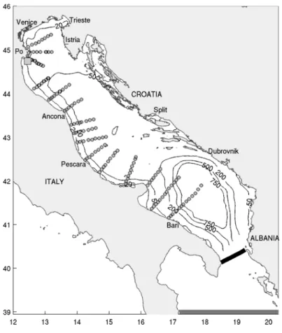
systems performance operating in the Adriatic Sea. The dataset consists of 150 CTD casts organised along 15 cross-shore sections (see Fig. 1), performed between 14 and 27 January 2006.

The full CTD dataset has been split in four sub-categories, depending on the depth of the sampling positions. The grouping has been done in order to evaluate scores

10

in different regions (from coastal to open sea). In general, regional forecasting sys-tems are built to provide more accurate “information” in the coastal zones that may be crudely represented in the large-scale system, therefore it is desirable understand if the regional systems add skills in such areas.

The regions have been defined as follows:

15

1. Very shallow region (group G1): casts on depths not exceeding 20 m. 2. Shallow region (G2): casts on depths between 20 and 50 m.

3. Mid-depth region (G3): casts on depths between 50 and 200 m. 4. Deep region (G4); casts on depths exceeding 200 m.

The quality of OOFS is usually assessed by means of basic statistics such as bias,

20

root mean squared error (RMSE), correlation coefficients and some skill scores (see Jolliffe and Stephenson, 2003, for a general review). Amongst these latter, one of the most used is probably the climatological skill score, or mean squared error skill score

(9)

OSD

3, 2087–2116, 2006

Adriatic Sea

Full Screen / Esc

EGU – MSESS (Murphy and Epstain, 1989), defined as follows:

MSESS = 1 − 1 n i =nP i =1 (mi − oi) 2 1 n i =nP i =1 (refi − oi)2 (1)

where m, o, ref , mean respectively model, observations and reference ith value, n the matched number of models-observations. In this case, the reference forecast in turn can be a climatology, persistence, or forecasts/analyses from another modelling

sys-5

tem. For sake of direct comparison between the regional and the large-scale systems, here the latter is used as reference in the MSESS estimates. Therefore, a positive (negative) skill score implies that the regional system is more (less) skilful compared to the large-scale reference system.

The comparison may appear somewhat unfair for the regional systems. MFS model

10

in fact does have data assimilation and flux correction (Demirov and Pinardi, 2002; Dobricic et al., 2006; Tonani et al., 20062) which should prevent drifts. The regional systems instead (continuous forecast and continuous hindcast) are free to evolve (and drift). On the other hand, a better performance of the latter at least on the coastal zone is still desirable.

15

A first general overview of the performance has been done by means of mean errors (ME) and RMSE. Scores are estimated interpolating model result in time and space on the CTD locations. Within each group all the differences model results-observations have been aggregated over time (in a quasi-synoptic assumption) and space before taking the mean and the root mean square.

20

Rating the relative performance compared to MFS, it has been chosen to estimate the skill score in each CTD location and then to compute the number of significantly

2

Tonani, M., Pinardi, N., Fratianni, C., and Dobricic, S.: Forecasting and analysis assess-ment through skill scores, in preparation, 2006.

(10)

OSD

3, 2087–2116, 2006

Adriatic Sea

Full Screen / Esc

positive, significantly negative and not-significantly different values within each group. Therefore a lager number of positive skill score suggest a relatively better performance. Significance of the score has been estimated using bootstrapping technique with 1000 re-samples. Results are summarised in Table 2.

Basically, with a few exceptions, all the models are fresher and colder than

observa-5

tions.

AdriaROMS shows a temperature mean RMSE of some 1◦_{C, irrespective the group.}

The ME instead has larger magnitude going toward deeper regions. AREG shows a mean RMSE higher than 1.3◦_{C in G1-G2-G3, while sensibly lower in G4. Better MEs}

are found in the very shallow and in the deep region. MFS has a similar behaviour, but

10

largest errors on the group G1.

Analysing the performance on salinity, the models have larger ME and RMSE in the very shallow group. This is easily explained by the difficulty to simulate the exact salin-ity in the western coastal current. Reasonably, errors get lower going toward deeper locations.

15

The comparison by means of MSESS shows that the regional systems have a larger number of positive scores in group G1, irrespective to the selected quantity. In the case of salinity, this may be counterintuitive since MFS has the lowest aggregated RMSE. Indeed, the RMSE is sensitive to extrema, and the aggregated RMSE for both AdriaROMS and AREG is somewhat downgraded by a low performance on a couple

20

of locations only. In general, both the regional systems show a good performance in the representation of the challenging very shallow coastal area, compared to the large scale system.

In the other groups the results are somewhat more regional model dependent. AdriaROMS performs better in temperature only, and excluded G4. G4 is somewhat

25

critical for this system, since this region (basically the deep southern Adriatic) is very close to the lateral open boundary and has a spatial resolution of about 10 km (coarser than MFS model).

(11)

oppo-OSD

3, 2087–2116, 2006

Adriatic Sea

Full Screen / Esc

EGU site behaviour between the two regional OOFSs).

Much of the performance depicted by the MSESSs in the coastal areas is likely as-sociated to biases. An example is provided in Fig. 2. The averaged vertical structures of AREG and AdriaROMS are consistent with the observations, leading to good results on linear association and amplitude error. On the other hand, the bias may be higher

5

eventually downgrading the performance on skill scores.

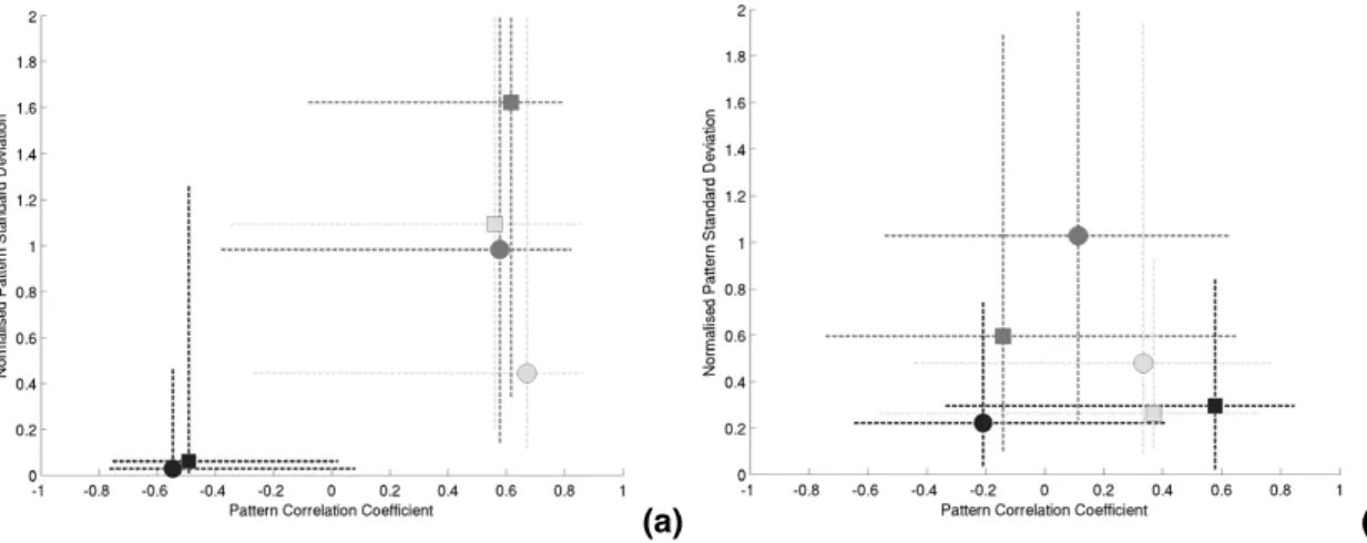
On the other hand, amplitude and phase errors of the regional OOFSs in the coastal CTD locations are different compared to those in deeper waters. A flavour of this be-haviour is show in Fig. 3a (grouping G1 and G2 together) and Fig. 3b (G3+G4). The figures show the median, the 25th and 75th percentiles of the sample distribution of

10

the centred (i.e., bias removed) standard deviation normalised by the standard de-viation of the observations and the pattern correlation coefficients (PCC). Regarding G1+G2, the correlations in both AREG and AdriaROMS are similar and reasonably high for temperature and salinity (the medians are some 0.6, even if the distributions is characterised by large spreading) with distribution of salinity in AREG and

tempera-15

ture in AdriaROMS centred on normalised standard deviation of unit (which is the most desirable value). Temperature in AREG instead often tends to overshoot the vertical stratification, while salinity in AdriaROMS to undershoot. The very low value of the medians for both normalised standard deviation and correlation in MSF suggest a low skill on reconstruction of the coastal gradients pattern, with the vertical profile being

20

actually too homogeneous and often not even linearly positively associated. Looking at the sample distributions in deeper regions (G3+G4), the overall performance of the regional models is downgraded. The medians of the pattern correlation coefficients are lower in AdriaROMS and even more in AREG. Now MFS model is instead more positively linearly associated at least on temperature profiles (in this region XBT

tem-25

perature data are assimilated). As a common feature, all the OOFSs tend to underesti-mate the amplitude of the profiles (with the exception of salinity in AREG), that is, a too homogeneous vertical profile. Along with the sample distribution of the correlations, the two regional systems depict a lower skill in reproducing the vertical stratification in

(12)

OSD

3, 2087–2116, 2006

Adriatic Sea

Full Screen / Esc

deeper region, whereas the performance of the large scale system gets slightly better compared to its performance in the coastal locations, at least regarding temperature.

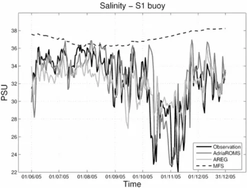
An additional example of the ability of the regional models to reproduce coastal gra-dients can be drawn by means of a comparison with buoy data available near the Po river mouth (Fig. 1), one of the most challenging locations from the point of view of

5

variability in salinity. This buoy, namely S1, provides hourly temperature and salinity data below the surface (0.5 m depth).

The comparison has been done on daily averages, therefore averaging to daily both buoy data and 3-hourly AdriaROMS results (AREG and MFS are already daily) before computing any statistics. Results are presented in Fig. 4. Beyond the obvious better

10

performance of the regional models (the large-scale models do not have any river implemented), it is noticeable the negligible ME even if with relatively high scatter (see Table 3 for ME and RMSE values). This behaviour is not found out for temperature, the three model performing nearly the same way (plot not shown, see Table 3 for statistics). In this case the crude representation of the Po river temperature flux (not included in

15

AREG and MFS, climatological in AdriaROMS) does not seem to impact that much on the performance.

In order to investigate the advantage of having different regional OOFS in the same area and to synthesise the operational systems results an additional analysis has been carried out combining PCC between models (PCCm), between model and

observa-20

tions (PCCo) and RMSE, grouping all the CTD casts. Results of the computation are shown in Fig. 5. On the base of PCC values four areas (A, B, C and D) have been de-fined: area A (high PCCm and low of PCCo values) identifies mutual systematic model errors; area B (high values of both PCCm and PCCo) indicates mutual skill; in area C (low values of both PCCm and PCCo) there are model-specific systematic errors

25

and finally area D (low PCCm and high PCCo values) states for model-specific skill. Some macro-proprieties of this analysis are: the two models have identical distribution between areas A and B; B is the most populated region while C is the area with less data.

(13)

OSD

3, 2087–2116, 2006

Adriatic Sea

Full Screen / Esc

EGU Considering both the models, we found that 73% of total population is within region

A and B, while 27% is in the regions C and D. The averaged RMSE in A+B is 0.97 while in C+D is about 1.19 with a total average (A+B+C+D) of 1.17. We can state that considering only the model solutions having positive PCCm improve the systems quality results of 17% in term of RMSE.

5

In the systematic error macro-region (A+C) there is a total population of 108 with 72 in the A area and 36 within C area. This means that most of the models error derives from mutual models proprieties. For example, the error can derive from physical assumption more than numerical technique used. This suggests that spending effort in improving the knowledge, and as consequence implement the correct physic, will give

10

more advantage than improve the numerical techniques.

The averaged RMSE in area B is 0.88 while in the region D it is about 1.16. There-fore, also considering only the model solution with positive PCCo (areas B–D) the portion of this population having positive PCCm also is generally a better estimation of the ocean state.

15

The 67% of model results with positive PCCm are characterized also by positive PCCo values, on the contrary only the 55% of models results with negative PPCm values show positive correlation with the observations. Having different models in the same region increase the confidence of models results also in terms of PCC.

4 Comparison with AVHRR SST

20

The observational dataset used in this section consists of one year of AVHRR com-posites providing sea surface temperature (SST). A daily SST map has been retrieved through the Pathfinder algorithm using composites of different night-time passages (Sciarra et al., 2006, and citation therein for details). Data are courtesy of ISAC-CNR Gruppo di Oceanografia da Satellite, Rome (IT). SST data have been provided with

25

clouds masked out and already mapped on AREG grid (approximatively 5 km resolu-tion) and for sake of comparison, AdriaROMS results have been bilinearly interpolated

(14)

OSD

3, 2087–2116, 2006

Adriatic Sea

Full Screen / Esc

onto the same grid. For equality of domains, this analysis has been limited to the south to the latitude 40.7 N.

The comparison between model SSTs and AVHRR skin SST may be critical when the warm layer develops and even worse in deeper regions (where the model surface temperature is indeed representative of a thick layer, because of the terrain following

5

vertical coordinate). The fact that SST images are night time does anyway help to minimise such biases.

MFS data are not considered in this analysis since these SSTs are used in the flux-correction procedure and therefore is not an independent dataset.

Based on this dataset, the RMSE has been computed on monthly, basin-wide,

aggre-10

gated subset of model outputs-observations. Compared to other possible approaches, for example first estimating over space the daily MSE and then averaging over time, this formulation permits to overcome the cloud-cover problem (it gives a lesser weight to days with less spatial coverage).

The RMSE estimated in the period June 2005–May 2006 are shown in Fig. 6. The

15

two regional OOFSs present indeed different scores, ranging roughly between 0.85 and 1.65◦_{C. AdriaROMS has a large RMSE seasonal cycle with high summer values}

while much better performance during winter. AREG shows better values during sum-mertime compared to wintertime, without a clear evidence of a seasonal cycle. In order to understand the source of the difference of this intra-annual behaviour, the

decom-20

position of the mean squared error has been carried out, following Oke et al. (2002) approach and nomenclature that is:

MS E = MB2+ SDE2+ 2SmSo(1 − CC) ; (2)

where MB= ¯m− ¯o is the mean bias, SDE=Sm−So is the standard deviation error,

(2SmSo(1−CC))

1

2 _{the cross correlation error, with m and o representing respectively}

25

model and observed values, S the standard deviation of the sample distributions, CC the correlation coefficients.

(15)

basin-OSD

3, 2087–2116, 2006

Adriatic Sea

Full Screen / Esc

EGU scale mean bias is roughly similar, except summer 2005. Such difference can be, at

least partly, explained by the use of daily averages as AREG SST, which would give a warm bias in summer. The correlation, ranging between 06–0.9, is roughly similar except in a few months. It seems indeed that the different seasonal behaviour is mostly controlled by the variations in the standard deviation error, or amplitude error, which in

5

its turn acts also in the cross-correlation error (in the term SmSo) leading this term to

a similar variability. Basically, the different seasonal behaviour is then associated to a larger range of large scale variability in AdriaROMS in summer, while larger in AREG in winter.

The fact that the mean bias between models is roughly similar is somewhat by

10

chance: in an intra-basin variability it is indeed different in magnitude, while the an-nual cycle (maximum in spring and minimum in fall) still holds. This can be noted in Fig. 8, where the monthly, zonal averaged mean bias is presented. The mean bias latitudinal displacement between the two models is in fact opposite. In AREG the main source of most negative biases is in the mid-northern part, in AdriaROMS is instead

15

the mid-southern, yet with a some positive biases in the northern. The reasons for that difference are potentially many, first of all the role of the different meteorological forc-ing, and only a dedicated process-study can elucidate the relative role of such driving mechanisms. In general, in AdriaROMS, the low performance in the southern region (which, by the way, is also consistent with previous results in G4 for January 2006) is

20

somewhat associated to a failure in the open boundary conditions, which posed the necessity to switch from clamped boundary conditions to radiation-relaxation, follow-ing Blayo and Debreu (2005). In AREG, part of the errors (in particular those at the latitude 44) are associated to horizontal diffusion problems (Oddo et al., 2005), yield-ing the spreadyield-ing of cold coastal waters inside the basin. These results are again

25

somewhat consistent with the performance in G2-G3, as well as the good results in the southern Adriatic which is consistent with the performance in G4.

(16)

OSD

3, 2087–2116, 2006

Adriatic Sea

Full Screen / Esc

5 Summary and conclusions

The regional operational forecasting numerical models, namely the AREG and Adri-aROMS systems, which cover the full Adriatic Sea region implemented during MFS project lifetime, have been presented and compared with the MFS model covering the entire Mediterranean basin and providing lateral boundary conditions data for the

re-5

gional models.

All the forecasting systems differ in operational suite, core ocean model, parameter-isation of the physics and meteorological forcing.

These operational systems performances have been evaluated by means of data-model and data-model-data-model comparison using standard statistics. Available observations

10

posed the limits of the comparison, which is in fact based on temperature and salin-ity and does not include any analysis on currents or other quantities. On the other hand, the dataset of observations include many source of data, such as CTDs, re-motely sensed sea surface temperature and data from one coastal buoy. This allowed having a full three-dimensional picture of the operational forecasting systems quality

15

during January 2006 and some preliminary considerations on the temporal fluctuation of scores estimated on surface or near surface quantities between summer 2005 and summer 2006.

Within the bounds posed by available observations, in the three-dimensional snap-shot of January 2006 the regional models has been found to be colder and fresher

20

than observations. Reasonably, both eventually outperform the large scale model in the shallowest locations. Performance on amplitude and phase errors are also much better in locations shallower than 50 m, while degraded in deepest locations, where the models tends to have a higher homogeneity along the vertical column compared to observations.

25

In a basin-wide overview, the two regional models show somewhat opposite local dis-placement of performances; AdriaROMS outperform the other models in temperature excluding the deepest, southern Adriatic, region, where AREG shows instead better

(17)

OSD

3, 2087–2116, 2006

Adriatic Sea

Full Screen / Esc

EGU results (as well as in salinity). This is also somewhat confirmed also by the comparison

with AVHRR SST.

At the same time, in locations where the regional models are mutually correlated, the aggregated RMSE has been found to be lower, which is a positive outcome of having several operational systems in the same region, as well as positive outcome is the

5

possibility to choose the best model given a certain area of interest, and nonetheless, the availability of having continuous real-time results which post processing procedure such as multi-model ensemble techniques may easily improve providing accurate real-time environmental pictures (Palmer et al., 2003; Krishnamurti et al., 2000). This work provided insights for the revision of the operational systems considered.

10

Acknowledgements. The authors greatly acknowledge ISAC-CNR Gruppo di Oceanografia da

Satellite for AVHRR and CTD data, ISMAR CNR Bologna for buoy S1 data. This work has been carried out within the framework of EU VFP MFSTEP project, as well as ADRICOSM project funded by the Italian Ministry of Environment and Territory (through the University of Bologna, Centro Interdipartimentale per le Ricerche di Scienze Ambientali, Ravenna, Italy) and

15

European INTERREG III CADSES – CADSELAND project. J. Chiggiato also acknowledge H. Arango, J. Wilkin (Rutgers University) and R. P. Signell, J. Warner (USGS) for useful hints during the implementation phase of AdriaROMS.

References

Blayo, E. and Debreu, L.: Revisiting open boundary conditions from the point of view of

char-20

acteristic variables, Ocean Modelling, 9, 231–252, 2005.

Blumberg, A. F. and Mellor, G. L.: A description of a three-dimensional coastal ocean circu-lation model, in: Three-dimensional coastal ocean models, edited by: Heaps, N. S., AGU, Washington D.C., 208 pp., 1987.

Budyko, K.: Climate and life, Academic Press, 508 pp., 1974.

25

Cushman-Roisin, B. and Naimie, C. E.: A 3D finite-element model of the Adriatic tides, Journal of Marine Systems, 37, 279–297, 2002.

(18)

OSD

3, 2087–2116, 2006

Adriatic Sea

Full Screen / Esc

its application to the Mediterranean Basin-scale Circulation, in: Ocean Forecasting, edited by: Pinardi, N. and Woods, J., 281–305, 2002.

Demirov, E., Pinardi, N., Fratianni, C., Tonani, M., Giacomelli, L., and DeMey, P.: Assimilation scheme of Mediterranean Forecasting System: Operational implementation, Ann. Geophys., 21, 189–204, 2003,

5

http://www.ann-geophys.net/21/189/2003/.

Demirov, E. and Pinardi, N.: Simulation of the Mediterranean Sea circulation from 1979 to 1993: Part I. The interannual variability, J. Mar. Syst., 33–34, 23–50, 2002.

Dobricic, S., Pinardi, N., Adani, M., Tonani, M., Fratianni, C., Bonazzi, A., and Fernandez, V.: Daily oceanographic analyses by the Mediterranean basin scale assimilation system, Ocean

10

Sci. Discuss., 3, 1977–1998, 2006,

http://www.ocean-sci-discuss.net/3/1977/2006/.

Fairall, C. W., Bradley, E. F., Rogers, D. P., Edson, J. B., and Young, G. S.: Bulk parameteri-zation of air-sea fluxes for Tropical Ocean Global Atmosphere Coupled-Ocean Atmosphere Response Experiment, J. Geophys. Res., 101, 3747–3764, 1996.

15

Flather, R. A.: A tidal model of the northwest European continental shelf, Memories de la Societe Royale des Sciences de Liege, 6, 141–164, 1976.

Joliffe, I. T. and Stephenson, D. B.: Forecast Verification; A Practitioner’s Guide in Atmospheric Science, John Wiley & Sons eds., 240 pp., 2003.

Krishnamurti, T. N., Kishtawal, C. M., Zhang, Z., LaRow, T., Bacjiochi, D., and Williford, E.:

20

Multimodel Ensemble Forecast for Weather and Seasonal Climate, J. Climate, 13, 4196– 4216, 2000.

Madec, G., Delecluse, P., Imbard, M., and L évy, C.: OPA 8.1 Ocean General Circulation Model reference manual, Note du P ôle de mod élisation, Institut Pierre-Simon Laplace, 11, 91pp., 1998.

25

Mellor, G. L. and Yamada, T.: Development of a Turbulence Closure Model for Geophysical Fluid Problems, Rev. Geophys. Space Phys., 20, 851–875, 1982.

Murphy, A. H. and Epstein, E. S.: Skill Scores and Correlation Coefficients in Model Verification, Monthly Weather Review, 119, 572–581, 1989.

Oddo, P., Pinardi, N., and Zavatarelli, M.: A numerical study of the interannual variability of the

30

Adriatic Sea (2000–2002), Science of the Total Environment, 353, 39–56, 2005.

Oddo, P., Pinardi, N., Zavatarelli, M., and Coluccelli, A.: The Adriatic Basin Forecasting System, Acta Adriatica, ADRICOSM Project special issue, in press, 2006.

(19)

OSD

3, 2087–2116, 2006

Adriatic Sea

Full Screen / Esc

EGU

Oke, P. R., Allen, J. S., Miller, R. N., Egbert, G. D., Austin, J. A., Barth, J. A., Boyd, T. J., Kosro, P. M., and Levine, M. D.: A modelling study of the three-dimensional continental shelf circulation off Oregon. Part I: Model-Data Comparison, Journal of Physical Oceanography, 32, 1360–1382, 2002.

Onken, R., Robinson, A. R., Kantha, L., Lozano, C. J., Haley, P. J., and Carniel, S.: A rapid

5

response nowcast/forecast system using multiply nested ocean models and distributed data systems, Journal of Marine Systems, 56, 45–66, 2005.

Palmer, T. N., Alessandri, A., Andersen, U., Cantelaube, P., Davey, M., D él écluse, P., D équ é, M., D´ıez, E., Doblas-Reyes, F. J., Feddersen, H., Graham, R., Gualdi, S., Gu ér émy, J.-F., Hagedorn, R., Hoshen, M., Keenlyside, N., Latif, M., Lazar, A., Maisonnave, E., Marletto, V.,

10

Morse, A. P., Orfila, B., Rogel, P., Terres, J.-M., and Thomson, M. C.: Development of a Eu-ropean Multi-Model Ensemble System for Seasonal to Inter-Annual Prediction (DEMETER), Bull. Amer. Meteo. Soc., 85, 853–872, 2003.

Pinardi, N., Allen, I., Demirov, E., De Mey, P., Korres, G., Lascaratos, A., Le Traon, P.-Y., Maillard, C., Manzella, G., and Tziavos, C.: The Mediterranean ocean Forecasting System:

15

first phase of implementation (1998–2001), Ann. Geophys., 21, 3–20 , 2003.

Raicich, F.: On the fresh water balance of the Adriatic Sea, Journal of Marine Systems, 9, 305–319, 1996.

Robinson, A. R. and Sellschopp, J.: Rapid assessment of the coastal ocean environment, in: Ocean Forecasting: Conceptual Basis and Applications, edited by: Pinardi, N. and Woods,

20

J. D., Springer-Verlag, NY, 199–229, 2002.

Sannino, G. T. M., Bargagli, A., and Artale, V.: Numerical modelling of the mean exchange through the Strait of Gibraltar, J. Geophys. Res., 107(C8), doi:10.1029/2001JC000929, 2002.

Sciarra, R., Bohm, E., D’Acunzo, E., and Santoleri, R.: The large scale observing system

25

component of ADRICOSM: the satellite system, Acta Adriatica, in press, 2006.

Shchepetkin, A. and McWilliams, J. C.: Quasi-monotone advection schemes based on explicit locally adaptive dissipation, Monthly Weather Review, 126, 1541–1580, 1998.

Shchepetkin, A. F. and McWilliams, J. C.: A method for Computing Horizontal Pressure-Gradient Force in an Oceanic Model with a Non-Aligned Vertical Coordinate, J. Geophys.

30

Res., 108, 3090, doi:10.1029/2001JC001047, 2003.

Shchepetkin, A. F. and McWilliams, J. C.: The Regional Ocean Modelling System: A Split-Explicit, Free-Surface, Topography-Following-Coordinate Oceanic Model, Ocean Modelling,

(20)

OSD

3, 2087–2116, 2006

Adriatic Sea

Full Screen / Esc

9, 347–404, 2005.

Smolarkiewicz, P. K.: A fully multidimensional positive definite advection transport algorithm with small implicit diffusion, J. Comput. Phys., 54, 325–362, 1984.

Steppeler J., Doms, G., Shatter, U., Bitzer, H. W., Gassmann, A., Damrath, U., and Gregoric, G.: Meso-gamma scale forecasts using the nonhydrostatic model LM, Meteorology and

At-5

mospheric Physics, 82, 75–96, 2003.

Zavatarelli, M. and Pinardi, N.: The Adriatic Sea Modelling System: a nested Approach, Ann. Geophys., 21, 345–364, 2003,

(21)

OSD

3, 2087–2116, 2006

Adriatic Sea

Full Screen / Esc

EGU Table 1. Summary of some of the most relevant differences amongst the three operational

forecasting systems.

OOFS MFS AREG AdriaROMS Dataset Analysis (weekly) Hindcast (weekly) Sequential forecast

(03:00–24:00) Horizontal resolution 1/16◦

(∼7 km) 5 km Variable (3 km ÷∼10 km)

Vertical Resolution 72 uneven z-coordinate

21 sigma coordi-nate

20 non linear s-coordinate

Output Daily averages Daily averages 3-hourly snapshots Initialisation Summer 2004 Spring 2003 Fall 2004

Domain Mediterranean Sea Adriatic Sea Adriatic Sea Meteorological forcing ECMWF analyses

(1/2◦_{, 6-hourly)}

ECMWF analyses (1/2◦_{, 6-hourly)}

LAMI forecasts (7 km, 3-hourly) Heat flux Computed w/flux

correction (SST from AVHRR) Computed w/out flux correction Computed w/out flux correction Fresh water flux Relaxation to

cli-matological SSS

Fresh water flux as salinity flux, all rivers but Po are climatological.

Only river flux (as source of mass and momentum); all rivers but Po are climatological Data Assimilation ARGO XBT SLA

(only XBT in the Adriatic region)

none none

(22)

OSD

3, 2087–2116, 2006

Adriatic Sea

Full Screen / Esc

Table 2. Mean error, root mean square error and mean square error skill scores in the four

groups G1, G2, G3, G4, divided by the range of depth of the CTD locations. SK+, SK-, SK? mean respectively the number of profiles in which the skill score is significantly positive (bet-ter the regional system), negative (bet(bet-ter the large scale system) or not significantly different (neutral). TEMP SALT ME RMSE SK+ SK- SK? ME RMSE SK+ SK- SK? AdriaROMS G1 0-20 0.09 1.03 16 4 1 -1.11 2.52 13 5 3 G2 20-50 -0.06 0.94 26 18 3 -0.54 0.72 4 40 3 G3 50-200 -0.73 0.98 30 26 2 -0.46 0.50 1 56 1 G4 200-inf -1.05 1.09 1 22 0 -0.34 0.34 0 23 0 AREG G1 0-20 -0.03 1.35 11 7 3 -0.75 1.97 11 7 3 G2 20-50 -0.96 1.65 15 23 9 -0.48 0.85 12 32 3 G3 50-200 -0.90 1.32 18 37 3 -0.58 0.66 2 54 2 G4 200-inf -0.02 0.25 16 7 0 -0.28 0.28 14 9 0 MFS G1 0-20 +1.13 1.97 +1.31 1.56 G2 20-50 -0.73 1.49 +0.11 0.54 G3 50-200 -0.76 1.25 -0.30 0.32 G4 200-inf -0.54 0.59 -0.31 0.31

(23)

OSD

3, 2087–2116, 2006

Adriatic Sea

Full Screen / Esc

EGU Table 3. Root mean square error and mean error of daily averages of temperature and salinity

at buoy S1 (respectively, TS1 and SS1). The period considered is from 1 July to 31 December 2005. AdriaROMS AREG MFS ME TS1 0.01 _−0.27 0.44 SS1 0.29 −0.17 4.82 RMSE TS1 1.23 0.93 0.85 SS1 2.73 2.41 5.95

(24)

OSD

3, 2087–2116, 2006

Adriatic Sea

Full Screen / Esc

Fig. 1. Adriatic Sea coastline and bathymetry. Location of the measurements used are also

shown: small circle are CTDs locations, light-grey square is S1 buoy. Note that iso-contour of depth 20 m, 50 m and 200 m, shown in the plot, are those used in the grouping done in Sect. 3.

(25)

OSD

3, 2087–2116, 2006

Adriatic Sea

Full Screen / Esc

EGU Fig. 2. Average profile for temperature (left panel) and salinity (right panel) of all the locations

(26)

OSD

3, 2087–2116, 2006

Adriatic Sea

Full Screen / Esc

(a)

(b)

Fig. 3. Sample distribution of normalized centred standard deviation and pattern correlation

coefficient of model vs. observations in group G1+G2 (a) and G3+G4 (b). Squares depict the median of the distribution of temperature, circles the median in case of salinity. Dashed lines shows the corresponding spread of 25th and 75th percentile. AdriaROMS is in light grey, AREG in medium grey, MFS in dark grey.

(27)

OSD

3, 2087–2116, 2006

Adriatic Sea

Full Screen / Esc

EGU

Figure 4:

(28)

OSD

3, 2087–2116, 2006

Adriatic Sea

Full Screen / Esc

Fig. 5. The x- and y-axes indicate vertical integrated PCC with observation (PCCo) and

be-tween models (PCCm) respectively while the colour indicates RMSE (models-observations) values. AdriaROMS values are shown with circle makers while AREG values with squared markers.

(29)